Environmental Pollution and Biodiversity: Light Pollution and Sea Turtles in
←
→
Page content transcription
If your browser does not render page correctly, please read the page content below
Environmental Pollution and Biodiversity:
    Light Pollution and Sea Turtles in the
                  Caribbeana

                                          Michael Brei
                               University Paris Ouest & SALISES

                                  Agustı́n Pérez-Barahonab
                                  INRA & École Polytechnique

                                           Eric Strobl
                                  École Polytechnique & IPAG

                                       January 25, 2014

                                             Abstract
           We examine the impact of pollution on biodiversity by studying the effect of
       coastal light pollution on the sea turtle population in the Caribbean. To this end
       we assemble a data set of sea turtle nesting activity and satellite derived measures
       of nightlights. Controlling for surveyor effort, local economic infrastructure and
       spatial spillovers, we find that nightlights significantly reduce the number of sea
       turtle nests. Using data on replacement costs of turtles raised in captivity, our
       result suggests that the increase in lighting over the last 20 years has resulted in
       the loss of close to 2,000 sea turtles in the Caribbean, worth up to $312 million.
       Incorporating our empirical estimate into a stage-structured population model we
       discover that the generational effects in the future are likely much larger. More
       generally, our study provides a new approach to valuing the cost of environmental
       pollution associated with species extinction.

       Keywords: biodiversity, pollution, sea turtles.
       Journal of Economic Literature: Q57

   a
      We would like to thank the members of the Réseau Tortues Marines Guadeloupe, particularly Eric
Delcroix, for sharing the data on sea turtle nesting, and Walter Mustin, Chief Research Officer of the
Cayman Turtle Farm.
    b
      Corresponding author: Department of Economics, INRA and Ecole Polytechnique, Avenue Lucien
Brétignière, 78850 Thiverval Grignon, France; e-mail: agperez@grignon.inra.fr.
1 Introduction
Over the last few decades, coastal areas have witnessed considerable growth in economic
activity (UNEP, 2008). Inevitably such growth has also been accompanied by significant
increases in environmental pollution, thus potentially threatening the rich biodiversity
that is characteristic of coasts (for instance, Jackson et al., 2001; and Myers and Worm,
2003). One important component of biodiversity is of course the protection of species
from exctinction (Polasky et al., 2005). A largely neglected aspect in this regard that has
drawn recent attention is the role that increased lighting due to local economic develop-
ment may play (Navara and Nelson, 2012; Gaston et al., 2013; and Kyba and Holker,
2013). More specifically, while a number of studies in the natural sciences have already
pointed out that some marine species are particularly sensitive to light pollution (see,
among others, Bustard, 1967; Witherington and Martin, 1996; and Bird et al., 2004),
the impact of the rising degree of coastal illumination has gone largely unexplored (Hill,
2006; Rich and Longcore, 2006; and USC, 2008). In this paper we set out to study how
light pollution in Caribbean coastal areas may have affected the critically endangered sea
turtle population (IUCN, 2001).1 In particular, light pollution in the Caribbean might
be an important threat for these species (Nicholas, 2001). Our aim here is to derive a
quantitative estimate of the impact of such pollution on sea turtle populations in the
region both in the short and long term.
A number of papers in the natural science literature have emphasized that the pres-
ence of nightlights likely interferes with sea turtle behavior in several ways. On the one
hand, artificial nightlight tends to deter sea turtle adults from nesting (Raymond, 1984;
Hirth and Samson, 1987; Witherington, 1992; and Johnson et al., 1996). At the same
time, it reduces the ability of sea turtle hatchlings to find their way from the beach
where they hatch to the sea, thus resulting in higher mortality rates due to exhaustion,
dehydration, and predation (Bustard, 1967; Tuxbury and Salmon, 2005; and Lorne and
Salmon, 2007). Nevertheless, the quantitative effect of nightlight on sea turtle nesting
and population has not yet been investigated statistically or limited to case studies of
particular beaches (Kaska et al., 2003; and Witherington and Frazer, 2003). The only ex-
ception in this regard is the study by Mazor et al. (2013), which investigates the effect of
satellite-derived nightlights on sea turtle nesting in the coastal areas of Israel. However,
although their descriptive statistics suggest a negative correlation between nightlights
and nesting activity2 , the authors find in the regression analysis that, peculiarly, the re-
lationship between nightlights and nesting is positive.3 Importantly though, they neither
control for surveyors’ effort nor for potential spatial spillovers between beaches, which as
1
In terms of the three turtle species examine here, both the green turtle (Chelonia mydas) and the
leatherback turtle (Dermochelys coriacea) were classified as endangered in 1996, while the hawksbill turtle
(Eretmochelys imbricata) was listed as endangered in 1986 but then upgraded to critically endangered
in 1996.
2
See Figure 3 and Table 2 of their paper.
3
See Table 3 of their paper. It is noteworthy that in an earlier study Aubrecht et al. (2010) also
noticed a positive relationship between nightlight intensity and the sea turtle nesting activity in Florida
in a simple plot of their data. However, as the authors argue, this counter-intuitive finding was likely
due to legislation in the mid-1980s which imposed regulation of beachfront lighting for the protection of
sea turtles in those beaches that were more lit.
1we show can bias the estimated impact. Moreover, they do not, as we do here, interpret
their quantitative estimates either in terms of the short or long term impact.
More generally speaking, there is a surprising paucity of solid statistical evidence of
the detrimental role that pollution may play in the loss of biodiversity or species extinc-
tion, despite the fact that it is widely recognized as one of the key threats to biodiversity4
and that it often enters public discourse in response to major pollution incidences such
as the Deepwater Horizon oil spill.5 The few papers that have examined this aspect have
been largely limited to the biology literature where the focus has been more generally
on how human population density may result in losses in biodiversity.6 The only ex-
ception in the economics literature is the study by Conrad (1989) who concludes that
the increased harvest of bowhead whales by Alaskian Eskioms threatened their existance.
Our paper contributes to the existing literature in a number of ways. First, we provide
a quantitative measure of how a potentially important type of pollution affects an endan-
gered species. More specifically, we estimate the impact of nightlight pollution on turtle
populations in Guadeloupe by combining data on satellite-derived nightlight images, the
location of sea turtle nesting sites, nesting activity, and local economic activity, as well as
surveyor effort. From a methodological point of view, we explicitly take into account the
spatial effects of nightlight pollution on sea turtle nesting in the context of count data
models. We then apply our estimates to a population model so as to capture the dynamic
implications of nightlights on the sea turtle population. To this end we incorporate our
estimates into a simulation of the sea turtle population dynamics for Guadeloupe using a
stage-structured population model as in Crouse et al. (1987) and Crowder et al. (1994).
Our approach follows Crowder et al. (1994) who investigate how turtle excluder devices
in trawl fisheries affect the sea turtle population in the Southeastern United States. How-
ever, in contrast to Crowder et al. (1994), we estimate rather than assume the impact of
our factor of interest on the population dynamics.
After controlling for local economic activity and the effort made in nest counting in
the econometric analysis, we find a significant negative impact of coastal nightlights on
the nesting activity of sea turtles in Guadeloupe. Other things being equal, we provide
evidence that a 1% increase of night illumination reduces the number of nests by around
6%. Moreover, we observe that the presence of marinas and hotels significantly deter sea
turtle nesting, while the proximity of roads and ports does not appear to be important
in our data. Extending our estimate of the marginal effect of nightlights to the whole
Caribbean, we find, as gauged from the cost of rearing sea turtles in captivity, that the
replacement of the nearly 2,000 “missing” sea turtles due to the greater night illumina-
tion since 1992 is up to 312 million US dollars. With respect to the impact of night
illumination on the future generations of turtles, we conclude from the calibrated pop-
ulation model that the fertility drop caused by photopollution substantially accelerates
4
See the Convention on Biological diversity at http://www.cbd.int.
5
The report of the Center for Biodiversity (April 2011) showed that more than 82,000 birds, 6,000
sea turtles, 26,000 marine mammals, and an unknown large number of fish and invertebrates may have
been harmed by the spill and its aftermath.
6
See, for instance, Luck (2007).
2the extinction of sea turtles. For hawksbill and green turtles, coastal nightlights decrease
the time of extinction from 164 and 154 years to 120 and 135 years, respectively. This
impact is even stronger for leatherback turtles, which under current light conditions will
eventually become extinct in 403 years. In contrast, if there was no light pollution then
the leatherback population would continuously increase in the long run.
The remainder of the paper is organized as follows. Section 2 reviews the literature
on the potential effects of light pollution on sea turtles. In Section 3 we describe our
database. The econometric methodology is introduced in Section 4 and the econometric
results are discussed in Section 5. In Section 6 we compute the replacement cost of the
missing turtles in the Caribbean, and in Section 7 investigate the population dynamics
and value its implications under different scenarios. Finally, Section 8 concludes.
2 Sea turtle nesting and nighlights
It is now widely accepted that coastal nightlights may deter sea turtles from nesting
(see, amongst others, Raymon, 1984; Witherington and Martin, 1996; Witherington and
Frazer, 2003; and Jones et al., 2011). More specifically, while sea turtles spend very
little of their life on beaches and almost exclusively at night, where females nest and
hatchlings emerge, these nocturnal activities are critical to the creation of future genera-
tions of turtles and may be significantly disturbed by the presence of night illumination.
Indeed, artificial lighting drastically alters the way adults choose their nesting sites as
they generally prefer unlit beaches (Raymond, 1984; and Witherington, 1992). Night
illumination also increases the possibility of direct human disturbance of nesting activity
(Carr and Giovannoli, 1957, and Carr and Ogren, 1960), frequently causing turtles to
abandon their nesting attempts (Hirth and Samson, 1987; and Johnson et al., 1996), or
to expedite the process of covering the eggs and camouflaging the nest site (Johnson et
al., 1996). Moreover, Witherington and Martin (1996) found turtles discarding their eggs
in the sea without nesting due to the lack of appropriate dark beaches. Photopollution
may also affect adult turtles’ return to the sea after nesting. Indeed, many experimental
studies show that adult turtles rely on brightness to spot the sea (Caldwell and Caldwell,
1962; Ehrenfeld and Carr, 1967; Ehrenfeld, 1968; Mrosovsky and Shettleworth, 1975).
However, this problem seems to be less severe than it is for the hatchlings (Witherington
and Martin, 1996).
Hatchlings emerge from eggs beneath the sand mainly at night and directly crawl to
the sea in order to increase their survival chances (Hendrickson, 1958; Bustard, 1967;
Neville et al., 1988; Witherington et al., 1990). However, by creating unnatural stimuli
light illumination can disrupt their instinctive sea-finding mechanisms, often resulting in
hatchling death due to exhaustion, dehydration, and predation. (see, for instance, Bus-
tard, 1967; and Witherington and Martin, 1996). It has been additionally observed that
indirect lighting can act as a perturbating factor by reflecting off buildings or trees that
are visible from the beach (Witherington and Martin, 1996). The sea-finding difficulties
of hatchlings together with the possibility of adult disorientation has led in some cases to
the replacement of the common blue light (shorter-wavelength) beach illumination with
3red light (longer-wavelength) lighting, since sea turtles are more sensitive to blue light.7
Nevertheless, such measures are frequently criticized because any luminary tends to en-
courage human activity on beaches (Witherington and Martin, 1996).
It is important to also point out that sea turtles exhibit natal philopatry which means
that females are likely to return to their natal beach for nesting. However, they may nest
in neighboring beaches if the original site is no longer suitable (e.g., Worth and Smith,
1976; Witherington and Martin, 1996). Nightlights may therefore have spatial spillover
effects: an illuminated beach may receive additional turtles because the neighboring nest-
ing sites are brighter. Not taking this into acount could thus lead to an underestimation
of any negative influence of light illumination.
3 Data description
3.1 Turtles nests
The sea turtle nesting data were provided by the Guadeloupe Sea Turtles Recovery Action
Plan.8 The survey identified a total of 156 nesting beaches in Guadaloupe, together with
their geolocation, of which 67 beaches were regularly surveyed for nesting activity at night
during the nesting season of 2008. The data consists of the number of nests, the number
of nights the beach was surveyed, and the sea turtle species of the nest. The species
indigenous to Guadeloupe are the green (Chelonia mydas), the hawksbill (Eretmochelys
imbricata), and the leatherback (Dermochelys coriacea) turtles. Summary statistics of
the nesting data, as well as all other variables used in our analysis, are provided in Table
A.1 of the Appendix. As can be seen, on average each beach was surveyed 40 times, with
a mean discovery of 26 nests, although there is considerable variation for both surveying
effort and nest discovery across beaches. One may also note that over half of the nests
found were for the hawksbill turtle.
3.2 Nightlights
In order to proxy nighttime illumination at the local level we resort to data derived from
satellite images of nightlights. More specifically, we use nightlight imagery provided by
the Defense Meteorological Satellite Program (DMSP) satellites. In terms of coverage
each DMSP satellite has a 101 minute near-polar orbit at an altitude of about 800km
above the surface of the earth, providing global coverage twice per day, at the same local
time each day. In the late 1990s, the National Oceanic and Atmospheric Administration
(NOAA) developed a methodology to generate “stable, cloud-free nightlight data sets
by filtering out transient light such as produced by forest fires, and other random noise
events occurring in the same place less than three times” from these data (see Elvidge et
al., 1997, for a comprehensive description). Resulting images are percentages of night-
light occurrences for each pixel per year normalized across satellites to a scale ranging
from 0 (no light) to 65 (maximum light). The spatial resolution of the original pictures is
7
For instance, the low-pressure sodium-vapor luminaries seem to affect nesting less than light from
other sources (Witherington, 1992).
8
See http://www.tortuesmarinesguadeloupe.org and Santelli et al. (2010) for further details.
4about 0.008 degrees on a cylindrical projection (i.e., with constant areas across latitudes)
and has been converted to a polyconic projection, leading to squares of about 1 km2 near
the equator. In order to get yearly values, simple averages across daily (filtered) values
of grids were generated. Data are publicly available on an annual basis over the period
1992-2010. 9
The nightlight image of Guadeloupe in 2008 is depicted in Figure 1. As can be seen,
there is an unequal distribution of nightlight intensity across the islands. More impor-
tantly, a large part of the brightness is concentrated near or on the coast.
Figure 1: Nightlights and nesting sites in Guadeloupe
3.3 Other data
We gathered information on the location of hotels and their capacity from a number of
sources, including http://www.guadeloupe-antilles.com, Google Maps and the individual
internet pages of the hotels. This resulted in a total of 69 hotels. The number of beds of
these range from 10 at Hostellerie des Chateaux to 1,316 at Club Mediterranee Caravelle.
In terms of ports and marinas we resorted to information at http://www.portbooker.com
and general internet searches. In this regard we identified and geo-localised the two main
ports of Guadeloupe and calculated the distance to the nearest port for each beach. With
respect to marinas there were a total of 24, ranging in size from 2 to 1,000 docks. As
a benchmark measure we summed the number of docks within 1 km of each beach. To
calculate out the distance to roads for our beaches we used the shape-files available at
http://www.diva-gis.org/gdata and the centroid of each beach.
9
One should note that a number of a papers now use nightlights as a proxy for economic activity;
see, for instance, Henderson et al. (2012). Here we use nightlights for what they are, namely a measure
of local light intensity during the night, while controling for economic activity in the area.
54 Econometric model
Given that our dependent variable is a count of the number of turtle nests, standard
linear regression techniques would not be appropriate. In terms of choosing the relevant
count data model one first needs to consider whether the data are characterized by over-
dispersion. Examining the summary statistics in Table A.1 this is clearly the case, as the
variance is substantially higher than the mean. When over-dispersion exists it is generally
preferable to use a negative binomial rather than the more common poisson count model.
However, importantly over-dispersion may also be caused by a large proportion of zeros
in the data, rendering traditional distributions insufficient to describe the data at hand.
Indeed in our data 27% per cent of nesting beaches were found to have no nesting activity.
We therefore follow Czado et al. (2007) and experiment with using the Zero-Inflated
Poisson and Zero-Inflated Generalized model. More specifically, the generalized Poisson
regression (GPR) model is given by:
yi
(1 + αyi )yi −1
µi −µi (1 + αyi )
f (µi , α, yi ) = exp , (1)
1 + αµi yi ! 1 + αµi
P
for yi = 0, 1, 2, . . .; where µi = µi (xi ) = exp( xij βj ), xi = (xi1 = 1, xi2 , . . . , xik ) is the
i-th row of covariate matrix X, and β = (β1 , β2 , . . . , βk ) is a k-dimensional column vector
of parameters. The mean of yi is given by µi (xi ). One should note that in equation
(1), the parameter α is a measures of dispersion, where if α > 0 then there is over-
dispersion, while if α = 0 the model reduces to a standard Poisson regression model. As
just noted, any over-dispersion due to an excess of zeros can be accounted for by using
the Zero-Inflated Poisson model:
P (Y = yi |xi , zi ) = ϕi + (1 − ϕi )f (µi , α, yi ), yi = 0
(2)
= (1 − ϕi )f (µi , α, yi ), yi > 0
where f (µi , α, yi ), yi = 0, 1, 2, . . . is the GPR model in (1), 0 < ϕi < 1 and ϕ(xi ). One
should note that the distribution of yi is characterized by over-dispersion when ϕi > 0
and that this model reduces to the zero-inflated Poisson model when α = 0. The mean
and variance of the count variable yi are given by:
E(yi |xi ) = (1 − ϕi )µi (xi ) (3)
and
V (yi |xi ) = (1 − ϕi )[µi 2 + µi (1 + αµi )2 ] − (1 − ϕi )2 µi 2
(4)
= E(y|xi )[(1 + αµi )2 + ϕi µi ].
As argued earlier, there is reason to believe that nesting behavior may be correlated
across space. One manner through which this can be modeled is the spatial correlation in
the error term. In doing so we follow Czado et al. (2007) and use a Gaussian Conditional
Autoregressive (CAR) formulation, which allows the modeling of spatial dependence, and
dependence between multivariate random variables at irregular spaced regions. More
specifically, for our set of J beaches {1, 2, . . . , J} we let γ = (γ1 , γ2 , . . . , γJ )t be the vector
of normally distributed spatial effects for each beach:
γ ∼ NJ (0, σ 2 Q−1 ) (5)
6
1 + |Ψ| · Ni i = j
Qij = −Ψ i∼j (6)
0 otherwise,
where Ni is the number of beaches within area i and ∼ indicates that i and j are neigh-
boring beaches. The conditional distribution of γi is then:
!
Ψ X 1
γi |γ−i ∼ N γj , σ 2 (7)
1 + |Ψ| · Ni j∼i 1 + |Ψ| · Ni
where γ−i are all the other values of γi . Importantly Ψ determines the degree of spatial
dependence, in that when Ψ = 0 there is no spatial dependence, but as spatial dependence
increases the value of Ψ will also be larger.
5 Econometric results
The results of estimating the determinants of nesting using the Zero-Inflated Generalized
Poisson model (ZIGP) are given in Table 1. One should note in this regard that we used
a Clarke test for all specifications to determine whether the model could be reduced to
a zero-inflated Poisson model by setting the over-disperson parameter α equal to zero.
As can be seen in Table 1, the resultant test statistic suggested that the ZIGP was the
preferred model in all specifications. In the baseline regression, shown in the first column,
we only include nightlights as an explanatory variable without any spatial effects. The
results suggest that the intensity of nightlights has a significant and negative effect on the
number of sea turtle nests. Since the ZIGP is a non-linear model, the coefficients have
no straightforward intuitive interpretation. Marginal effects for any explanatory variable
xk with estimated coefficient βk are thus calculated as follows:
∂Nests X
= βk exp β1 + βj · xj , (8)
∂xk
where β1 is the constant coefficient in ourPregression, xj denotes the average of xj , and
the terms inside the summation operator refer to the explanatory variables found to
be significant. The marginal effects of the significant coefficients are given in Table 2.
Accordingly, the estimated coefficient in our base specification suggests that a one unit
increase in nightlights reduces the number of nests by 3.8. As noted earlier, one concern
is that sea turtle nesting behavior may be spatially correlated. In the second column of
Table we thus allow for spatial correlation of the error term as outlined above. In this
regard, we as a benchmark considered beaches within 5km of each other as neighbors.
As can be seen, the positive and significant estimate of Ψ suggests that the data does
indeed exhibit spatial dependence across neighbors. The marginal effect, as gauged from
the second column in Table 2, is now somewhat lower, standing at -2.2 nests, than
without spatial correlation. We thus continue allowing for spatial effects in the remaining
specifications.10
10
As can be seen throughout Table 1, the spatial effects are always found to be statistically significant.
7Table 1: Determinants of sea turtle nesting activity
(1) (2) (3) (4) (5) (6)
Nightlights -0.0735 -0.0909 -0.0894 -0.0869 -0.0868 -0.0924
(-0.1281, -0.0259) (-0.1517, -0.0210) (-0.1658, -0.0110) (-0.1379, -0.0284) (-0.1489, -0.0134) (-0.1704, -0.0059=)
Effort 19,3983 14.3023 24.7793 17.7003
(12.4168, 32.4372) (8.6860, 23.6536) (10.5916, 33.5149) (1.8344, 28.4067)
Roads -0.3405 -0.1121 -0.4351
(-0.9545, 0.3221) (-0.7751, 0.8339) (-3.4642, 0.8692)
Marinas -0.0237 -0.0282 -0.0368
(-0.0377, -0.0060) (-0.0402, -0.0035) (-0.0663, -0.0002)
Hotels -0.0053 -0.0057 -0.0227
8
(-0.0060, -0.0042) (-0.0067, -0.0024) (-0.0263, -0.0053)
Distance to port -0.0004 -00041 -0.0069
(-0.0008, 0.0000) (-0.0048, -0.0000) (-0.0091, 0.0029)
Spatial parameter 1.3654 7.0969 3.8690 2.6935 1.5540
(0.1604, 4.6391) (1.6764, 15.8881) (1.2483, 8.7586) (0.6313, 6.7299) (0.1100, 4.3290)
Constant 4.7348 4.1349 4.4418 5.3409 4.5363 5.4483
(3.2526, 5.9300) (3.2008, 4.7707) (2.8292, 5,8064) (3.1082, 7.2999) (2.1336, 6.2304) (2.7065, 7.9775)
Observations 67 67 67 67 67 67
Clarke test:
ZIP 0.1623 0.0055 0.0524 0.0070 0.0524 0.0020
No decision 0.0874 0.1568 0.1688 0.2088 0.1329 0.2143
ZIGP 0.7318 0.8272 0.7567 0.7687 0.7952 0.7537
Notes: (1) The 5th and 95th confidence interval are given in parentheses; (2) The Clarke test reports the proportion of decisions in favour of each
model.Table 2: Marginal effects for significant coefficients
Specification: (1) (2) (3) (4) (5) (7)
Nightlights -3.8331 -2.1627 -5.9272 -5.7968 -6.9318 -3.4624
Effort – – 1.2857 0.9542 1.9787 6.6306
Roads – – – – – –
Marinas – – – -1.5824 -2.2517 -1.3778
Hotels – – – -0.3521 -0.4223 -0.8497
Ports – – – – – –
Importantly the number of nests discovered on a beach is likely to depend on the
effort made by those counting. Moreover, one could very well imagine that perhaps
greater effort is undertaken in those beaches that are better lit, thus potentially biasing
the negative effect of nightlights downward. We thus in the third column include our
effort intensity measure.11 Unsurprisingly, greater surveying effort increases the number
of nests being discovered, where the marginal impact of one unit greater monitoring in-
tensity is associated with the discovery of one additional nest. Comparing the marginal
effects of lighting from the specification without to that with the effort dummy, shows
that there is indeed a downward bias, where for the latter the reduction per unit of night-
light is nearly three times larger.
Nightlight intensity itself may be correlated with a number of other features of local
economic activity that may affect a sea turtle’s decision to nest at a particular beach.
For example, beaches are usually more lit the closer they are to hotels, but having ho-
tels nearby will likely also increase the probability of nesting activity being disturbed
by tourists. Similarly, local shipping activity might disturb nesting near beaches, and
such activity tends to be higher at ports which are also more lit than, ceteris paribus,
those without ports nearby. To ensure that the estimated effect of nightlight intensity
is not capturing these other local features, we included the total number of hotel beds,
the number of docks, and the number of ports within a 1km radius of the beach, as well
as the distance to the nearest road. As can be seen in the fourth column of Table 2,
ports and roads have no significant effect on nesting. In contrast, one finds that both the
greater number of docks and the greater number of hotel beds nearby reduce the number
of nests found on a beach. In terms of their marginal effects our coefficients imply that,
for example, 10 additional beds in nearby hotels decrease the number of nests by 3.5,
whereas a dock present within 1km of the nesting beach reduces nests by 1.58.
Our analysis can also be done by sea turtle species. More specifically our sample
consists of 59% hawksbill, 38% green, and 3% leatherback nests. Given the small sample
size of leatherback nests, the estimation of the spatial model was not feasible for these,
and we only re-estimate the full specification of column (4) for hawksbill and green turtle
nests; see columns (5) and (6), respectively. Reassuringly nightlights significantly deter
11
Note that, for ease of presentation, our variable effort ẽ is in per thousand units of the original
one e (i.e., ẽ = e/1000). Therefore, the marginal effect of the original effort variable is ∂Nests/∂e =
∂Nests/∂ẽ · dẽ/de, where ∂Nests/∂ẽ is provided by (8) and dẽ/de = 1/1000.
9nesting for both species. The inferred marginal effects indicate that the impact of an
additional unit of nightlight on nesting activity is larger for the hawksbill than for the
green turtle.
Thus far we have controlled for spatial effects only via the error term. Feasibly,
however, there also may be spatial effects in terms of the covariates. For instance, with
regard to the main focus of this study, a greater brightness of nearby beaches may have
positive spillover effects on a local beach, as discouraged turtles look for alternative
nesting sites nearby. To investigate this we calculate the average nightlight intensity of
beaches within 5km, excluding a beach’s own value. Similar measures were defined for
the distance to road, docks, ports and hotel bed variables. The results, see Table A.2 in
the Appendix, indicated that there are no direct spatial spillover effects of the nightlight
intensity of nearby beaches. Similar conclusions were reached when we extended the
proximity threshold to 10km.
6 The “missing” sea turtles in the Caribbean
In the previous section we provided a quantitative estimate of the negative impact of light
pollution on sea turtle nesting, taking account of other potentially confounding factors
and spatial correlation. Apart from the arguable interest in the actual number itself,
one can also use it to derive a monetary interpretation of our estimate for the wider
Caribbean. To this end we would have ideally liked to expand our econometric analysis
above for the entire region. However, unfortunately we were not able to obtain nesting
activity data for other territories. We thus instead assume that the case of Guadeloupe
is representative of the Caribbean and use our econometric estimates to infer the total
costs of the reduction in sea turtle nests due to nightlight pollution.
As a proxy of the monetary value of “missing” sea turtles due to nightlight pollution
we use known costs of rearing sea turtles in captivity, an approach that has been used
to infer the minimum value of the ecological services provided by sea turtles (see, for in-
stance, Freeman, 2003; and Troeng and Drew, 2004), particularly if there are no specific
estimates for willingness to pay available.12 To identify the nesting beaches in the entire
Caribbean we used information from SWOT/OBIS-SEAMAP, which provides a list of
known nesting sites and their location.13 The 1,086 known nesting beaches along with
nightlight intensity during 2010 are depicted in Figure 2.
12
One should note that in our case we would need a willingness to pay (WTP) measure per individual
turtle. As far as we are aware, the only WTP for sea turtles are those that refer to particular conservation
programs - see, for example, Jin et al. (2010) -, and are not individual specific.
13
SWOT - the State of the World’s Sea Turtles - is a partnership led by the Sea Turtle Flagship
Program at the Oceanic Society, Conservation International, IUCN Marine Turtle Specialist Group, and
supported by the Marine Geospatial Ecology Lab at Duke University. See SWOT (2006, 2008, and 2009).
10Figure 2: Nesting sites in the Caribbean
Note: Green dots indicate known nesting sites.
Accordingly, the location of nesting beaches and their nocturnal illumination varies
widely across the Caribbean. Moreover, there has been an increase in nightlight intensity
in most nesting beaches over time, as can be seen from Figure 3 which plots 1992 against
2010 nightlight intensity for each nesting site.
Figure 3: Light pollution at nesting sites in the Caribbean: 1992 vs. 2009
60 40
Nightlights 2010
20 0
0 20 40 60
Nightlights 1992
With the change in nightlight intensity for each beach and our measurement of the
marginal effect of nightlights in hand, one can estimate the number of missing turtles as
11follows:
1086
X ∂Nests Hatchlings
∆Nightlightsi × × × survival rate to adulthood. (9)
i=1
∂Nightlights Nest
The first term represents the overall change in nightlight intensity on the nesting beaches
over the period 1992-2010. For this we summed total net changes in illumination for all
nesting beaches, which we found to be 2,811 units of light (i.e., a 16% increase of 1992
intensity). For the marginal change in nests due to light pollution we used the estimated
marginal effect for all turtles from our econometric analysis, i.e., -5.8. These two figures
together suggest that the number of missing nests over our sample period is 16,304. With
regard to the average number of eggs per nest, while this varies across species and loca-
tion, it is about 120. Finally we assume that the survival rate of hatchlings is equal to
1/1000; see, for instance, Frazer (1986). Equation 9 then implies that there were 1,957
missing sea turtles due to nightlight intensity over our sample period.
Regarding the monetary valuation of the missing turtles, we need the cost of rearing
sea turtles in captivity. For this we resort to estimates derived from case studies of turtle
farms and marine conservation centers. In this regard, we took information from three
sources: Troeng and Drews (2004) for green and leatherback turtles, Webb et al. (2008)
for hawksbill turtles, and, from a personal communication with the Cayman Turtle Farm
in the Cayman Islands, for green turtles. We summarize the replacement costs in Table
3 (see Appendix B for further details):14
Table 3: Replacement costs per species (in US dollars)
Farm Species Cost/15-years Cost/adult Replacement costs
old in millions
Ferme Corail green 1,672 3,455 6.7
Cayman Turtle Farm green 4,185 8,649 16.9
WMI Research facility hawksbill 18,045 26,466 51.8
TUMEC, Rantau Abang leatherback 112,128 159,504 312.1
Source: own calculations.
One striking aspect of these figures is that the costs of raising a leatherback turtle in
captivity until 15 years of age and adulthood are multiple times larger than the equivalent
figures for green and hawksbill turtles. However, the leatherback is also the largest of
the three, with a carapace length between 1.30 and 1.83m and a weight between 300 and
500kg. In contrast, green sea and hawksbill turtles are considerably smaller with, respec-
tively, a carapace length of 83-114cm and 71-89cm and normally weighing 110-190kg and
46-70kg (Marquez, 1990).
14
We assume that green sea turtles reach adulthood at the age of 31 (Cambell, 2003), while the
equivalent is 21 for the leatherback type (Martinez et al., 2007; and Saba et al., 2012) and 22 for the
hawksbill turtles (Crouse, 1999).
12Combining the cost per individual adult with our estimate of missing turtles we then
calculate the total replacement cost of missing turtles. According to our estimates, shown
in the last column of Table 3, this ranges from 6.7 million to 312.1 million US dollars,
depending on the relative importance of each species nesting in the Caribbean.15 In other
words, the cost of replacing the implied number of missing turtles with animals raised
in captivity could be as much as 0.3 billion US dollars if these were mostly leatherback
turtles. It is important to emphasize, as argued by Freeman (2003) and Troeng and
Drews (2004), that the replacement cost as measured here should only be considered as a
lower threshold of the true loss in ecosystem services since it ignores externalities arising
from sea turtles being raised in their natural environment.
7 Population dynamics
In the previous section, making use of our econometric estimate of the negative impact
of light pollution on sea turtle nesting, we have quantified and valued the number of
“missing turtles” due to nighttime illumination in the Caribbean. These results however
only take into account a single generation of turtles, neglecting any population dynamics.
The aim of this section is to incorporate the generational effects by means of integrating
our estimate into a population dynamics model.
Mathematical biology is plentiful of sophisticated population models (see, amongst
others, Cushing, 2006; and Wikan, 2012). Nevertheless, the calibration of these models
is often constrained by the availability of data. The reproduction and survival rates, for
instance, play a key role in these dynamical settings. In the context of sea turtles it is
well-known that these figures are age-dependent. It is thus argued that age-structured
models, like the one introduced by Leslie (1945), would be an appropriate framework to
study the population dynamics of sea turtles. Unfortunately, there is little reliable age-
specific information for long-lived iteroparous species, such as the sea turtles. Still, since
the life cycle of sea turtles is composed of a series of well-identified stages (see Heppell
et al., 2003, for a introduction to the ecology of sea turtle population), more information
is available regarding the duration, survival, and reproduction rates of each stage. We
thus follow the setup introduced by Lefkovicth (1965), Crouse et al. (1987), and Crowder
et al. (1994), where individuals are grouped by stage instead of age, sharing the same
reproduction and survival rates.
7.1 Stage-structured population model
As in Crowder et al. (1994), we consider five stages of development for the sea turtles,
namely, eggs/hatchlings (1), small juveniles (2), large juveniles (3), subadults (4), and
adults (5). We then define the stage distribution vector xt at time t as
xt = (x1t , x2t , x3t , x4t , x5t ), (10)
15
Unfortunately there are no available estimates of nesting activity by species available for the
Caribbean.
13where xit is the number of female turtles in the i-th stage at time t, for i = 1, . . . , 5. Let
us also denote Pi as the percentage of females in the i-th stage that survive but remain in
the i-th stage, Gi as the percentage of females in the i-the stage that survive and progress
to the next stage, and Fi as the number of hatchlings per year produced by a sea turtle
in the i-th stage (annual fecundity). Therefore, the number of hatchlings produced by
each stage class at time t is given by:
x1t = F 1 x1t−1 + F 2 x2t−1 + F 3 x3t−1 + F 4 x4t−1 + F 5 x5t−1 , (11)
while the number of females present in the subsequent j-th stage, for j = 2, . . . , 5, is:
xj t = Gj−1 xj−1 t−1 + P j xj t−1 . (12)
Taking (11) and (12), we can then rewrite our population model in matrix form:
xt 0 = Lxt−1 0 , (13)
where x0 denotes the transpose of vector x, and L is the five-stage population matrix
F1 F2 F3 F4 F5
G1 P2 0 0 0
L= 0 G2 P 3 0 0 .
0 0 G3 P4 0
0 0 0 G4 P5
In general, the available stage-based life information for sea turtles is comprised of dura-
tion and survival and reproduction rates. The fertility rates Fi are given by the fecundity
data, while Gi and Pi need to be calculated. In this regard, we follow the standard method
of Crouse et al. (1987) and Crowder et al. (1994). If we denote the yearly survival rate
of sea turtles in stage i and the duration of the i-th stage by σi and di , respectively, one
can then determine the percentage of sea turtles from stage i that grow into stage i + 1
(γi ) as:
(1−σi )σidi−1
d if σi 6= 1
γi = 1−σi i (14)
1
di
if σ = 1. i
Consequently, the percentage of turtles in stage i that remain in the i-th stage is 1 − σi .
We can finally determine Gi and Pi as:
Gi = γi σi (15)
Pi = (1 − γi )σi . (16)
7.2 Population dynamics and nightlight pollution
As pointed out above, the usual stage-based life table for a specific type of sea turtle
consists of information about the duration, survival and reproduction rates of each stage.
14We provide in Appendix C the corresponding stage-based life tables for the nesting types
of sea turtles in Guadeloupe. Considering (14)-(16), we can then compute the population
matrix L for each species. With this matrix in hand, taking (13) and an initial stage
distribution vector x0 , we obtain the population dynamics for t ≥ 0.
Let us now incorporate the effect of night illumination into the population model.
As we have shown earlier, nightlight pollution significantly reduces the number of sea
turtle nests and, consequently, the annual fertility per turtle. The objective then is to
adjust the parameter Fi to account for the marginal effect of nightlights. One should
note that an additional negative consequence of nightlights is the increasing difficulty of
hatchlings to find the sea after emerging from their nest, resulting in a reduction of their
annual survival σ1 (see Section 2). Our analysis should thus be interpreted as a lower
bound of the negative effect of nightlight pollution, although we do later investigate how
incorporating this aspect would affect our results.
As a starting point we assume nightlight intensity and nesting activity to be the
average observed on Guadeloupe nesting beaches, and denote these as N Lavg and N T avg ,
respectively. In order to modify the annual fertility we essentially need to estimate the
reduction of hachlings per year caused by nightlights. Thus, the average percentage
reduction in the nests τ due to the night illumination is:
|β1 |N Lavg
τ (β1 ) = 100, (17)
N T avg + |β1 |N Lavg
where β1 denotes the estimated marginal negative effect of light pollution.
With no available empirical evidence to resort to, we assume that the percentage
reduction in nests will result in the same percentage reduction in eggs per sea turtle. Since
we are working at the individual marine turtle level, we will adjust the marginal effect
of nightlights to take account of the remigration interval, which we, following Doi et al.
(1992), assume to be 2.6 years implying that β˜1 = β1 /2.6.16 The modified annual fertility
can therefore be computed as F̃i = [1 − τ (β˜1 )/100]Fi . Recall that the marginal effect
for the hawksbill and green turtles is -6.93 and -3.46, respectively. For the leatherback
turtle we assume that the marginal effect is simply equally to the sample average of -5.8.
Thus for the leatherback turtle the annual fertility would reduce by 47%, changing the
population matrix accordingly. Note that our analysis is based on a constant level of
nightlights per beach since our objective is to evaluate the generational consequences
of the current level of light pollution. The set-up, however, could be easily applied to
evaluate different scenarios of nightlight changes.
7.3 Dynamic population response
We can now evaluate the population dynamics under a scenario with and one without
night pollution. One can obtain the population dynamics for each turtle type, starting
16
Other studies on remigration intervals include Carr and Carr, 1970; Carr et al., 1978; Hays, 2000;
and Troeng and Chaloupka, 2007).
15from a given initial stage distribution by recursively applying equation (13) to the pop-
ulation matrix with and without nightlights. Given that the data on the number and
stage distribution of sea turtles is very uncertain due to the difficulties in tracking sea
turtles, we assume an initial number of turtles for each stage which is consistent with
broad estimates for Guadeloupe (see, amongst others, DREG (2008) and Delcroix et al.
(2011)). More precisely, we assume for each type of turtle a population of 1,000 females
per stage. Nevertheless, we verified that the qualitative population response is robust to
alternative demographic configurations.17
7.3.1 Population dynamics
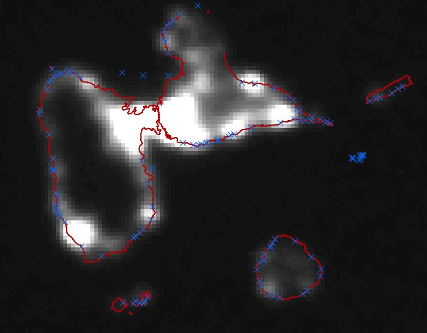
In Figures 4-6 we plot the evolution of the stage population for each type of sea turtle,
with and without nightlights. As can be seen, even without light pollution both the
hawskbill and the green sea turtle eventually become extinct, while the population of the
leatherback continues to grow over time. One should note that this difference in the long-
term population dynamics across species is in line with existing studies18 and is driven
by the underlying survival and fertility parameters of the population matrix. However,
as is also clear from the figures, the presence of nightlights considerably accelerates the
process of extinction for hawksbill and green turtles. For the leatherback turtle the neg-
ative impact of nightlights reverses population growth so that these also become extinct
in the long run.
Figure 4: Population per stage – hawksbill turtle
Hatchlings (LHS) 100 Hatchlings (LHS)
Small juveniles (LHS) 1.4 Small juveniles (LHS) 1.4
100
Large juveniles (LHS) Large juveniles (LHS)
Subadults (RHS) Subadults (RHS)
Adults (RHS) 1.2 Adults (RHS) 1.2
80
80
Number of turtles (thousand)
Number of turtles (thousand)
Number of turtles (thousand)
1.0 1.0 Number of turtles (thousand)
60
60 0.8 0.8
0.6 0.6
40
40
0.4 0.4
20 20
0.2 0.2
0 0.0 0 0.0
0 10 20 30 40 50 60 70 0 10 20 30 40 50 60 70
Years Years
(a) no nightlights (b) nightlights
17
Details are available from the authors upon request.
18
For instance, Evans et al. (2001).
16Figure 5: Population per stage – green turtle
Hatchlings (LHS) Hatchlings (LHS)
100 Small juveniles (LHS) 100 Small juveniles (LHS)
Large juveniles (LHS) 1.5 Large juveniles (LHS) 1.5
Subadults (RHS) Subadults (RHS)
Adults (RHS) Adults (RHS)
80 80
Number of turtles (thousand)
Number of turtles (thousand)
Number of turtles (thousand)
Number of turtles (thousand)
1.0 1.0
60 60
40 40
0.5 0.5
20 20
0 0.0 0 0.0
0 10 20 30 40 50 60 70 0 10 20 30 40 50 60 70
Years Years
(a) no nightlights (b) nightlights
Figure 6: Population per stage – leatherback turtle
Hatchlings (LHS) Hatchlings (LHS)
Small juveniles (LHS) Small juveniles (LHS)
100 Large juveniles (LHS) 1.5 100 Large juveniles (LHS) 1.5
Subadults (RHS) Subadults (RHS)
Adults (RHS) Adults (RHS)
80 80
Number of turtles (thousand)
Number of turtles (thousand)
Number of turtles (thousand)
Number of turtles (thousand)
1.0 1.0
60 60
40 40
0.5 0.5
20 20
0 0.0 0 0.0
0 10 20 30 40 50 60 70 80 0 10 20 30 40 50 60 70 80 90
Years Years
(a) no nightlights (b) nightlights
Figures 4 and 5 clearly show that the population of hawksbill and green turtles is
always greater without nightlights than under night illumination. Moreover, one should
also note from Figure 6 that the negative effect is more pronounced for the leatherback
type. As a matter of fact without light pollution the population of leatherback turtles
would increase in the long-run.
One should note that the qualitative population dynamics do not depend on the initial
stage distribution. Indeed, the eigenvalues of the population matrix allow us to identify
the dynamic properties regardless of the initial conditions. An intrinsic characteristic of
17the population model here is that population either increases or decreases in the long
run, since the model consists of a system of first-order linear difference equations. One
can easily verify, see Appendix D, that the absolute value of all eigenvalues of the pop-
ulation matrices for hawksbill and green turtles are lower than one. Consequently, their
population will be asymptotically extinct regardless of the presence of light pollution.
For the leatherback type, however, there is an eigenvalue (λ1 ) greater than one if there is
no nightlight pollution, so that its population increases in the long-run. As for hawksbill
and green turtles, nightlights result in all eigenvalues being lower than one, leading to
the eventual depletion of this species too. As pointed out earlier, there are of course
more sophisticated frameworks that consider non-linearities which induce steady popu-
lations. This is usually the case of models that incorporate the effect of agglomeration
by allowing, for instance, for food and/or space competition among individuals. Even if
the data required to estimate a model of this type were available, the existence of such
agglomeration effects seems unlikely for endangered species like the sea turtle.
The eigenvalues also allow us to provide quantitative information regarding the long-
run response of the population of each type of turtle and, in particular, its growth rate
and stage distribution. Since the system (13) has constant coefficients and |λ1 | > |λj | for
j = 2, . . . , 5 (see Table A.7), the unique solution in the long-run takes the form:
xt 0 ≈ c1 λ1 t vλ1 , (18)
where vλ1 is the eigenvector corresponding to the eigenvalue λ1 , and c1 is a constant.19
Consequently, the long-run annual growth rate of the population (per stage and total) is
equal to λ1 − 1. Applying this result to our simulations, we observe that the population
eventually decreases for both hawksbill and green turtles, but that nightlights increase
the long-run annual depletion from 7.19 to 10.18 % and from 7.9 to 8.76 %, respectively.
We also confirm that the population of the leatherback type increases if there is no light
pollution, with a long-run annual growth rate of 1.07%. However, the presence of night
illumination reverses this trend, resulting in an eventual decreasing population at a rate
of 2.75% per year.
With respect to the stage distribution of each type of turtle, using equation (18) the
long-run proportion of population in the i-th stage is given by:
vλ
ξi = P5 1 i , (19)
k=1 vλ1 k
where vλ1 k is the k-th coordinate of the eigenvector vλ1 . Considering the eigenvalues and
eigenvectors of tables A.7 and A.8 in Appendix D, we obtain the stage distribution for
each type of turtle with and without nightlights. A well-known feature of these kinds
of population models is that the population reaches a stable stage distribution in the
long-run – see Table A.9 and Figures A.2 in Appendix D. As is evident from Table
A.9, the proportion of hatchlings is most severely affected by nightlight pollution. The
P5 t
19
The solution of the system (13) for all t is xt 0 = i=1 ci λi , where vλi denotes the eigenvector
corresponding to the eigenvalue λi of the population matrix, and ci are constants determined by the
initial population distribution.
18reduction is particularly apparent for the leatherback where the proportion of hatchlings
falls by more than 3 percentage points, and it is a major reason for why the population
reverses from its increasing long-run trend. These results are robust to the initial stage
distribution and other population sizes, because there are strong accumulative effects of
the reduction in annual fertility.
The population model can be applied to study how fast this extinction may occur.
More specifically, let us define the time to extinction te as the number of years it takes
for less than one turtle to remain. Table 4 shows for our initial population of p0 = 5, 000
turtles that night illumination significantly accelerates the extinction of all three species.
Without nightlight pollution the hawksbill and green turtles will take 164 and 154 years to
become extinct, respectively. In the case of leatherback there is in contrast no extinction
but rather an ever increasing population size. In the presence of nightlights eventually all
three species will disappear. According to our simulations, the years of extinction now
are 110 years for the hawksbill, 135 years for the green and 403 years for the leatherback.
Thus night illumination on nesting sites has a clear accumulative effect in the long-run
driven by the reduction in fertility rates of adult females.20
Table 4: Time of extinction (in years)
no light light light (σ̃1 )
Hawksbill 164 110 90
Green 154 135 119
Leatherback – 403 186
Our estimates of the impact of nightlights are likely to be only lower bounds as we do
not allow for the fact that, due to disorientation, lighting will also reduce the number of
hatchlings that make it from the nesting site to the sea. Unfortunately we do not have
any information of the impact of nightlights on the survival rate of hatchlings during
this period of their life cycle in our data. However, Peters and Verhoeven (1994) studied
loggerhead hatchling survival from their nests to the sea. More specifically, they examine
two nesting sites on the Turkish Mediterranean coast and found that on the one that was
well lit only 21% of hatchlings reached the sea, as compared to an adjacent unlit area
where the success rate was 48%. In order to get a rough feel of how far our estimates are
from the upper bound, we modify our hatchling survival probability as σ˜1 = 0.56σ1 .21
As expected, extinction accelerates. More precisely, the time to extinction for hawksbill
and green turtles is now 90 and 119 years, respectively, while for the leatherback it would
take 186 years to extinction, see Table 4.
Finally, Figures 4-6 shown above reveal that the short-run population dynamics are
cyclical. This property is explained by the fact that sea turtles spend several years in each
20
Note that the time of extinction depends on the distribution and size of the initial population,
however, the qualitative results remain unchanged when we use alternative scenarios.
21
The 56% is just the percentage reduction in the survival rates as found by Peters and Verhoeven
(1994).
19stage of development, resulting in the accumulation or reduction of number of individuals
in a specific stage. This result is confirmed by examining the eigenvalues of the population
matrix (see Table A.7).22 Moreover, the negative effect of light pollution does not seem
to be strong enough to eliminate these cycles in the short-term.
7.3.2 Compensation costs
One conservation management tool used to address a diminishing species’ population that
has been employed in the case of sea turtles is that of headstarting, where headstarting
broadly entails the captive hatching and rearing of sea turtles through an early part of
their life cycle.23 For instance, the Cayman Turtle Farm has over the period 1980 to 2001
released a total of 16,422 neonates, 14,282 yearling and 65 older (19-77 months) green sea
turtles.24 As a simple thought experiment we can use our results above to consider the
costs of using such a headstarting strategy to counteract the negative effect of nightlights
on sea turtles.
We can use our results above to consider the costs involved in using headstarting to
compensate for the accelerating effect of nightlights on sea turtle extinction. Our thought
experiment in this regard consists of calculating the number of headstarted turtles that
would have to be released into the wild today to keep the time of extinction the same
as without nightlight pollution.25 We can then infer an estimate for the potential cost
of such a conservation strategy using our information on the costs incurred in raising
turtles in captivity. As mentioned before, headstarted turtle have been release at various
life stages, normally well before they reach the age of 7 years. Moreover, since we do
not have information on the replacement costs of hatchlings, we here limit our analysis
to the release of headstarted, one year old small juveniles. For the green turtle, we find
that 5.5 million small juveniles would be needed to keep the time to extinction at the
no nightlights level of 154 years with an associated cost between 0.6 and 1.5 billion dol-
lars, depending on which source we use for the yearly replacement cost. In the case of
the hawksbill, 130 million yearlings would have to released in order to keep the time to
extinction at the no nightlight level of 164 years, with an associated cost of 156 billion
dollars.
At first sight the compensating costs involved with using headstarting as a conser-
vation management tool may seem remarkably high. However, one needs to remember
that we are considering counteracting the negative effect of nightlights over all the years
until extinction. Moreover, in line with arguments made by Heppel et al. (1996) in terms
of using headstarting to compensate for reduced survival rates, these large figures are
also due to the characteristics of the sea turtle itself. First, for a slow maturing species
like sea turtles, large increases of juveniles are needed to compensate for the reduction in
22
The existence of complex and/or negative eigenvalues implies short-run cycles in difference equation
systems.
23
See, amongst others, Bell et al. (2005).
24
Other examples include the North Carolina Head Start program (loggerhead turtles) and National
Marine Fisheries Service Program (kemp’s ridley turtles).
25
One should note that we are considering here only a one-time injection of sea turtles, however, the
exercise could of course be extended to yearly release programs.
20nesting activity and hence hatchling production due to light pollution. Secondly, except
for extremely small populations, it is unfeasible to headstart enough juveniles to have an
impact on the overall survival rate of a cohort.
Finally, it is important to also point out that there are other likely costs involved
with headstarting; see Bell et al. (2005) for a review. Firstly, turtles raised in captivity
may behave differently than those from the wild. For example, there is some evidence
that headstarted turtles forage and nest outside of their natural range. Others have
also questioned the ability of headstarted sea turtles to survive as well as wild ones
due to nutritional deficiencies and behavioural modifications as a consequence of insuf-
ficient exercise, lack or inappropriate stimuli, and unavailability of natural food sources
and feeding techniques during captivity. Additionally, headstarted sea turtles may have
negative spillovers on wild sea turtles via the transmission of diseases acquired during
captivity and genetic pollution. Thus, as large as they are, in actuality the cost estimates
that we provide here should only viewed be as a lower bound of the total costs of us-
ing headstarting as remedy for the detrimental sea turtle population effects of nightlight
pollution.
8 Concluding remarks
We examine the loss of biodiversity due to environmental pollution by studying the im-
pact of coastal light pollution on the sea turtle population in the Caribbean. To do
so we assembled a data set of sea turtle nesting activity and satellite derived measures
of nightlights for Guadeloupe. Using a spatial count data model we show that, after
controlling for surveyor effort and local economic infrastructure, nightlights reduced the
number of nests on beaches. Considering the growth of nightlights over the last 20 years
across beaches known to be used for nesting in the Caribbean, our quantitative estimate
suggests that if we consider the value of a sea turtle to be that of its replacement cost
in captivity, then the increase in coastal lighting in the region has resulted in losses of
up to 520 million US dollars. We then combine our statistical estimate within a stage-
structured population model for Guadeloupe to study the generational implications of
light pollution. The results suggest that light pollution substantially accelerates the ex-
tinction of sea turtles. Moreover, we find that compensating the negative effect of the
current nightlight intensity by means of rearing sea turtles in captivity and then releasing
them into the wild, as is part of some current conservation strategies, may be an expen-
sive remedy. This suggests that one should explore what the economic costs of reducing
coastal illumination near sea turtle nesting beaches as an alternative or supplementary
conservation management tool would be.
More generally, our paper arguably provides a new approach to valuing the loss in
species extinction due to environmental pollution. In particular, given data on a species
of interest and some type of relevant pollution, our paper shows that using statistical
estimates of the short-term impact within a population model can provide helpful insight
into at least the range of the likely long-term impacts and their costs. Obviously how
reliable such predictions might be will depend on the quantity and quality of data avail-
21You can also read