Determining reservoir intervals in the Bowland Shale using petrophysics and rock physics models
←
→
Page content transcription
If your browser does not render page correctly, please read the page content below
Geophys. J. Int. (2022) 228, 39–65                                                                                     https://doi.org/10.1093/gji/ggab334
Advance Access publication 2021 August 20
GJI Rock and Mineral Physics, Rheology

Determining reservoir intervals in the Bowland Shale using
petrophysics and rock physics models

Iain Anderson ,1 Jingsheng Ma,1 Xiaoyang Wu2 and Dorrik Stow1
1 Instituteof GeoEnergy Engineering (IGE), School of Energy, Geoscience, Infrastructure & Society, Heriot-Watt University, Edinburgh, EH14 4AS, UK.
E-mail: i.anderson@hw.ac.uk
2 British Geological Survey, The Lyell Centre, Research Avenue South, Edinburgh, EH14 4AP, UK

Accepted 2021 August 13. Received 2021 July 14; in original form 2021 January 6

                                                                                                                                                             Downloaded from https://academic.oup.com/gji/article/228/1/39/6355446 by guest on 08 October 2021
                                        SUMMARY
                                        An evaluation of prospective shale gas reservoir intervals in the Bowland Shale is presented
                                        using a wireline log data set from the UK’s first shale gas exploration well. Accurate identi-
                                        fication of such intervals is crucial in determining ideal landing zones for drilling horizontal
                                        production wells, but the task is challenging due to the heterogeneous nature of mudrocks.
                                        This heterogeneity leads to stratigraphic variations in reservoir quality and mechanical prop-
                                        erties, and leads to complex geophysical behaviour, including seismic anisotropy. We generate
                                        petrophysical logs such as mineralogy, porosity, and organic content and calibrate these to the
                                        results of core studies. If ‘reservoir quality’ is defined by combined cut-offs relating to these
                                        parameters, we find that over 100 m of reservoir quality shale is present in the well, located
                                        primarily within the upper section. To examine the link between geophysical signature and
                                        rock properties, an isotropic rock physics model is developed, using effective medium theo-
                                        ries, to recreate the elastic properties of the shale and produce forward-looking templates for
                                        subsequent seismic inversion studies. We find that the mineralogical heterogeneity in the shale
                                        has a profound impact on modelled elastic properties, obscuring more discrete changes due
                                        to porosity, organic content and water saturation and that the best reservoir quality intervals
                                        of the shale bear a distinctive response on rock physics cross-plots. Finally, we consider the
                                        density of natural fractures in the shale by developing an anisotropic rock physics model to
                                        reflect high-angle fractures observed on micro-imagery logs. We invert crack density using
                                        shear wave splitting well log data and find a crack density of up to 4 per cent which cor-
                                        relates well with micro-imagery observations. Our work further supports previous authors’
                                        core-based studies in concluding that the Bowland Shale holds good reservoir characteristics,
                                        and we propose that there are multiple intervals within the shale that could be targeted with
                                        stacked horizontal wells, should those intervals’ mechanical properties also be suitable and
                                        there be adequate stress barriers between to restrict vertical hydraulic fracture growth. Finally,
                                        our rock physics templates may provide useful tools in interpreting pre-stack seismic data sets
                                        in prospective areas of the Bowland Shale and picking the best locations for drilling wells.
                                        Key words: Elasticity and anelasticity; Microstructure; Europe; Downhole methods; Acous-
                                        tic properties; Seismic anisotropy.

                                                                                microscale such as mineralogical heterogeneity, multiscale layer-
I N T RO D U C T I O N
                                                                                ing and natural fractures. These textures can cause complex geo-
The concept of tight mudrocks forming commercially viable hy-                   physical behaviour, such as anisotropy as observed in ultrasonic
drocarbon reservoirs was first realized in the USA during the early             laboratory studies (Jones & Wang 1981; Vernik & Nur 1992; Son-
21st century, and their successful exploitation has since revolution-           dergeld et al. 2000), wireline velocity logging (Esmersoy et al.
ized the energy industry. However, mudrocks or shales, pose unique              1994; Walsh et al. 2007; Horne et al. 2012) and reflection seis-
challenges to hydrocarbon production. Low matrix permeability ne-               mology (Johnston & Christensen 1995; Bakulin et al. 2000a, b;
cessitates the use of stimulation techniques such as hydraulic frac-            Sayers 2005).
turing to unlock isolated hydrocarbons from their micro/nanoscale                  The Mississippian Bowland Shale Formation of north England
pores and they often exhibit complex textures at the macro- and                 is considered the best candidate for shale gas extraction in the

C The Author(s) 2021. Published by Oxford University Press on behalf of The Royal Astronomical Society. This is an Open Access

article distributed under the terms of the Creative Commons Attribution License (https://creativecommons.org/licenses/by/4.0/), which
permits unrestricted reuse, distribution, and reproduction in any medium, provided the original work is properly cited.
                                                                                                                                                        39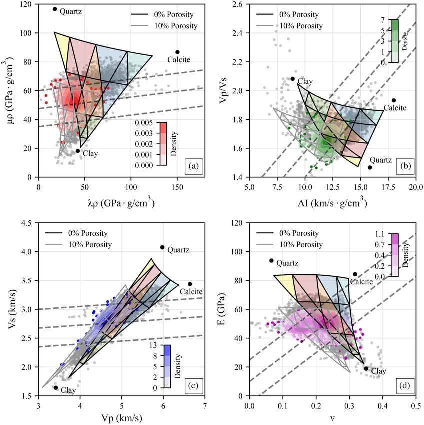
40      I. Anderson et al.

United Kingdom (Smith et al. 2010), though the size of the po-             high Caliper values indicating washout within the associated shales
tential resource is disputed (Andrews 2013; Whitelaw et al. 2019).         (not shown in Fig. 2). The Upper Bowland Shale (UBS) displays
Exploration thus far has focused within the Craven Basin of NW             clear heterogeneity shown by the varying GR response. An increase
England, where the Bowland Shale exhibits excellent shale reser-           in Uranium Concentration (GRUR) near the top of the UBS sug-
voir properties (Clarke et al. 2014a, 2018) and has been subject           gests an enrichment in organic matter. Further washout sections
to several sedimentological and microstructural studies (Fauchille         evidenced by very low RHOB values exist but are confined to thin
et al. 2017; Newport et al. 2018; Emmings et al. 2019, 2020a,b,c).         intervals. The Lower Bowland Shale (LBS) displays a different char-
However, the geological structure of the Craven Basin is complex,          acter; one of alternating thicker high GR units interbedded with low
and the shale resource is compartmentalized by high-angle reverse          GR units. The low GR units belong to the Pendleside Sandstone
faults into narrow blocks (Anderson & Underhill 2020). This com-           Member, and while these are relatively thin in the PH-1 well, they
partmentalization suggests that long (>2 km) horizontal wells (as          can reach up to 300 m thickness in the Clitheroe area (Clarke et al.
are traditionally used in shale gas plays) may not be possible in          2018). Three of the LBS high GR units (shales) were penetrated
this area. Furthermore, all hydraulic fracturing attempts have re-         before the well reached total depth.
activated either seismic-scale or subseismic-scale faults, leading to
elevated levels of induced seismicity and premature halting of oper-
ations (Clarke et al. 2014b, 2019b; Kettley & Verdon 2021; Kettlety

                                                                                                                                                     Downloaded from https://academic.oup.com/gji/article/228/1/39/6355446 by guest on 08 October 2021
                                                                           Lithological heterogeneity in the Bowland Shale
et al. 2021).
   This faulting may necessitate the use of shorter horizontal wells       The wireline log signature of the Bowland Shale is one character-
targeting different stratigraphic intervals (‘stacked’ lateral wells) to   ized by variability in rock properties and this is owed, in part, to
produce commercial volumes of gas from the Bowland Shale. Such             the mineralogical heterogeneity of the formation. The heterogeneity
a technique would ensure that as much shale could be stimulated            observed can be related to the complex and dynamic relationship
as possible, whilst optimizing the horizontal well trajectories away       between tectonic and sedimentary processes active during depo-
from mapped faults. Production from the Bowland Shale using                sition of the shale (the Visean and Namurian periods). The LBS
stacked lateral wells has been briefly mentioned in the literature         is a hemipelagic mudstone that accumulated during the Visean
(Clarke et al. 2014a, 2018) but without detailed analysis detailing if     within several isolated syn-rift basins separated by shallow plat-
multiple prospective intervals exist in the shale and how they may         forms on which extensive shelf carbonates were deposited (Fraser
be targeted. Selecting the best intervals to target with horizontal        & Gawthorpe 1990; Corfield et al. 1996). During this time, the car-
wells ultimately requires knowledge of the reservoir quality and           bonate platforms were flanked by reefs that effectively cut the supply
geomechanical characteristics of the shale formation.                      of detrital carbonate into the basins, leading to the development of
   In this work, we address the issue of selecting the best reservoir      a dysaerobic, stratified water column (Kirby et al. 2000). As a re-
quality (RQ) intervals for stacked drilling at the well Preese Hall-1      sult, LBS mudstones are typically calcareous, locally organic-rich
(PH-1) by using petrophysical and rock physics analysis. We fo-            and predominantly reflect low-energy turbidite deposition (Newport
cus specifically on characterizing the Bowland Shale’s mineralogy,         et al. 2018). The thick low GR units observed at the base of PH-1
organic content, porosity, permeability and water saturation from          are coarse sandstones of the Pendleside Sandstone Member (Fig. 2)
wireline logs. We then implement two rock physics models; first,           (Clarke et al. 2018) which represent higher-energy turbidites, pos-
an isotropic model to assess the link between rock properties and          sibly sourced from coastal deltas to the north (Kirby et al. 2000).
isotropic elastic properties, and secondly an anisotropic model to            The boundary between the LBS and UBS is taken at the Visean-
invert natural fracture density from shear splitting logs. We then         Namurian boundary which also marks a change in regional tectonics
conclude by presenting a classification of the intervals that hold the     from syn-rift to post-rift subsidence (Fraser & Gawthorpe 1990).
best RQ and consider how these might be predicted from seismic             Throughout the Namurian period, the deltas already established in
data.                                                                      the Midland Valley of Scotland and NE England prograded south-
                                                                           wards and their influence was reflected in the progressive infilling
                                                                           of the previous syn-rift depocentres (including that of the Craven
                                                                           Basin) with increasingly coarse clastic material (Fraser et al. 1990;
B A C KG R O U N D
                                                                           Fraser & Gawthorpe 2003). In PH-1, the Namurian UBS consists
                                                                           predominantly of mudstone with varying silt content, thin sand-
PH-1 lithostratigraphy and wireline character
                                                                           stones and thin dolomitized limestones (Clarke et al. 2018). Marine
The PH-1 well was drilled by Cuadrilla Resources between 16th              transgressions (‘marine bands’) are a prominent feature and are vis-
August and 3rd December 2010 in the Fylde region of Lancashire,            ible on the wireline logs as thin, high GR intervals. Emmings et al.
NW England (Fig. 1). As it was designed with the purpose of shale          (2020a) observed these features in adjacent boreholes and outcrops
gas evaluation, several specialized wireline logging runs (Table 1)        confirming these as pelagic/hemipelagic carbonate and fossil-rich
and core studies (Table 2) were undertaken, and these data sets            mudstones.
were accessed for this study via the British Geological Survey. It            This macroscale heterogeneity in lithology types described above
encountered the Bowland Shale at 1980 m TVD-MSL (True Vertical             also manifests at microscale. A range of microtextures (relating to
Depth below Mean Sea Level), and drilled through 725 m of the              the degree of lamination and/or predominant mineralogy), organic
formation before reaching total depth at 2730 m TVD-MSL.                   matter types and fracture styles have been characterized within
   The shallowest wireline logging at PH-1 is within the Sherwood          samples taken from PH-1 cores (Fauchille et al. 2017, 2018) and
Sandstone (Fig. 2). The Manchester Marl is characterized by very           those authors suggest that depositional variability is a strong control
low Gamma Ray (GR), low Bulk Density (RHOB) and high Deep                  on the heterogeneity observed. Taking these multiscale observations
Resistivity (DDLL) zones indicative of evaporites. Very low RHOB           of rock character together, it is apparent that the Bowland Shale is a
values and high Compressional (DTC) and Shear (DTS) Sonic                  mineralogically and texturally complex formation. It is important to
Slowness readings within the Millstone Grit are accompanied by             define how this heterogeneity influences reservoir and geophysical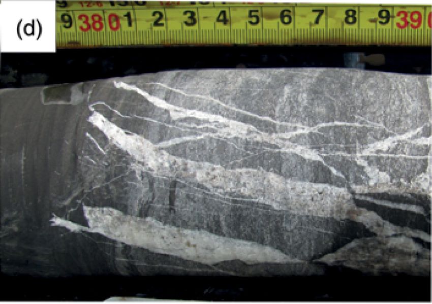
Bowland Shale Reservoir Intervals              41

                                                                                                                                                          Downloaded from https://academic.oup.com/gji/article/228/1/39/6355446 by guest on 08 October 2021
Figure 1. Two-way-time structure map for the Lower Bowland Shale on the Fylde region highlighting the Preese Hall-1 (PH-1) well, additional wells and
interpreted faults (after Anderson & Underhill 2020). GH-1Z, Grange Hill-1Z; Th-1, Thistleton-1; PNR, Preston New Road-1; El-1, Elswick-1; RW, Roseacre
Wood.
Table 1. Summary of wireline logs and typical bed resolutions acquired at PH-1 and accessed for this study (Contains OGA Well Log
                                                                                                                                  C Data accessed and

published with permission of BGS).
Logging run                       Tool assemblage                     Typical bed resolution        Key logs
Intermediate (561–1390 m)         Sonic Quad Combo                           ∼30 cm                 Compressional Sonic, Neutron Porosity, Gamma
                                                                                                    Ray, Bulk Density, Laterolog Resistivity, Caliper,
                                                                                                    Photoelectric absorption
TD (1371–2781 m)                  Sonic Quad Combo                           ∼30 cm                 Compressional Sonic, Neutron Porosity, Gamma
                                                                                                    Ray, Bulk Density, Laterolog Resistivity, Caliper,
                                                                                                    Photoelectric absorption
                                  Dipole Sonic                               ∼1.4 m                 Compressional Slowness, Fast Shear Slowness, Slow
                                                                                                    Shear Slowness, Fast Shear Azimuth, Anisotropy
                                  Compact Micro-Imager                       ∼0.5 cm                Microresistivity array, four-arm caliper
                                  Spectral Gamma Ray                         ∼30 cm                 Uranium Concentration, Potassium Percentage,
                                                                                                    Thorium Concentration
42      I. Anderson et al.

          Table 2. Summary of PH-1 core laboratory results used for this work. The tests were commissioned by Cuadrilla Resources and are
          presented in the PH-1 End of Well Report (Contains OGA Well Log C Data accessed and published with permission of BGS).

          Laboratory tests                                    Rock properties                                         Number of samples
          X-ray diffraction (XRD)                             Mineralogy                                                      88
          Mercury Immersion and Helium Pycnometry             Porosity, permeability and water saturation                     48
          Source Rock Analayser - Pyrolysis                   TOC                                                             96

properties as this will in turn influence the placement of horizontal              Furthermore, there is some evidence that these sub-vertical fea-
wells.                                                                          tures correspond to shear-wave anisotropy. This anisotropy is char-
                                                                                acterized by the cross-dipole sonic tool, which measures the shear-
                                                                                wave splitting (SWS) effect; where the shear-wave is polarized into
                                                                                fast and slow shear waves upon entering an anisotropic medium (Liu
Seismic anisotropy in the Bowland Shale                                         & Martinez 2012). As this polarization can often be attributed to
                                                                                the presence of aligned fractures in the logged formation (Esmersoy
An important phenomenon when considering the geophysical
                                                                                et al. 1995), it has become a popular tool for unconventional reser-

                                                                                                                                                         Downloaded from https://academic.oup.com/gji/article/228/1/39/6355446 by guest on 08 October 2021
behaviour of shale is anisotropy in elastic properties. Seismic
                                                                                voir characterization. SWS can also be used to determine fracture
anisotropy can be most simply defined as the ‘dependence of seismic
                                                                                sets from reflection seismic (Davis et al. 2003; Shuck et al. 1996),
velocity upon angle’ (Thomsen 2002). The phenomenon is caused
                                                                                vertical seismic profiles (Winterstein et al. 2001) and microseismic
by the preferential alignment of minerals, pores, or fractures. It is
                                                                                events (Verdon et al. 2009; Verdon & Kendall 2011).
particularly acute in mudstones as they are deposited in low-energy
                                                                                   While shear anisotropy is generally low at PH-1, locally high
settings (giving rise to sedimentary processes that produce lami-
                                                                                values can be observed in areas where subvertical fractures and/or
nated textures), significantly compacted during burial (accentuating
                                                                                wider fracture zones are present (Fig. 4). These manifest as high
alignment of pores and minerals) and often extensively fractured at
                                                                                amplitude sinusoids on the micro-imagery log and chaotic zones
multiple scales (such as exhibiting microfractures due to hydrocar-
                                                                                without clear character (Figs 4b and c). However, the greatest shear
bon generation, or macrofractures due to burial diagenesis). A ma-
                                                                                wave anisotropy readings appear to correspond to zones of induced,
terial with anisotropic elastic properties is theoretically represented
                                                                                rather than natural fractures, which produce symmetrical, borehole-
in Hooke’s Law by a complex, fourth-rank elastic stiffness tensor of
                                                                                parallel high conductivity features that cut across bedding (Fig. 4a).
81 independent parameters (Mavko et al. 2009). However, in prac-
                                                                                In each case, the presence of subvertical features approximately nor-
tice, a plane of symmetry is often imposed, allowing the tensor to
                                                                                mal to bedding can be taken as evidence of HTI behaviour, which is
be significantly reduced to a manageable five constants. Therefore,
                                                                                then quantified by the shear wave anisotropy log. However, the im-
shale is commonly referred to as transversely isotropic with either
                                                                                pact of drilling-related features can clearly overprint the anisotropy
a vertical plane of symmetry (VTI, i.e. fabric is bedding-parallel)
                                                                                response caused by natural fractures and thus these zones need to
or transversely isotropic with a horizontal plane of symmetry (HTI,
                                                                                be treated with caution.
i.e. fabric is bedding-normal). Voigt notation is commonly used to
                                                                                   As discussed previously, VTI anisotropy is also known to be
represent the elastic stiffness tensor (cij ), which for a transversely
                                                                                prevalent in shales due to the presence of bedding-parallel features
isotropic (TI) medium is (Mavko et al. 2009):
                                                                                (e.g. laminated clays or aligned kerogen and/or pores). However,
       ⎛                                       ⎞                                there is no clear evidence to suggest that this is a significant phe-
         c11 c12 c13          0      0      0
       ⎜c12 c11 c13           0      0      0⎟                                  nomenon in the Bowland Shale. Clarke et al. (2019a) show how
       ⎜                                       ⎟
       ⎜c13 c13 c33           0      0      0⎟                                  micro-imagery log data can be used to identify strong layering of
ci j = ⎜
       ⎜0
                                               ⎟,
       ⎜         0     0     c44     0      0⎟ ⎟
                                                                                shales and carbonates but also conclude that both the anisotropy
       ⎝0        0     0      0     c44     0⎠                                  wireline log data and the ultrasonic velocity experiments demon-
          0      0     0      0      0    c66                                   strate negligible anisotropy in elastic properties. Fauchille et al.
                                                                                (2017) highlighted the presence of a ‘strongly laminated’ facies in
                                   1
                     where c66 = (c11 − c12 )                       (1)         the shale and identified bedding-parallel microcracks filled with bi-
                                   2                                            tumen which all may influence seismic anisotropy, but at present,
   While there is limited data to confirm that seismic anisotropy may           there is no data to quantify the degree of influence.
be a strong feature of the Bowland Shale, aligned fabrics within the               Further work is needed to determine the effect of VTI fabrics
shale have been documented in some studies. One such fabric is                  on the anisotropy of the Bowland Shale. Ultrasonic velocity exper-
the presence of natural fractures, which are a common feature to                iments conducted on core samples oriented at different angles to
shale plays (Gale et al. 2014) and are prevalent in the PH-1 well.              bedding/lamination would be required to fully quantify the degree
Some of these are open, but many are mineral (usually calcite)-filled           of TI anisotropy. For an accurate characterization, measurements
and are usually oriented perpendicular or at high angles to bedding             on three core plugs (oriented normal to, 45◦ to and parallel to bed-
(Fauchille et al. 2017; Clarke et al. 2018), suggesting HTI behaviour.          ding) are required (Vernik & Nur 1992). However, the preparation
Clarke et al. (2018) demonstrate how these can be observed on core              of such samples (particularly those at 45◦ to bedding) can be chal-
samples (Fig. 3b) and thin sections, whereas Fauchille et al. (2017)            lenging due to shale’s friability, which led Wang (2002) to propose
identify them using SEM images (Fig. 3c). These fractures are                   a method whereby transducers could be placed at different orienta-
also of sufficient aperture to be imaged on micro-imagery log data              tions to bedding on a single sample. However, both these methods
and can be identified as the presence of either bright (i.e. resistive,         require access to core samples of sufficient size to obtain a large
healed) or dim (i.e. conductive, open, fluid-filled) sinusoids usually          plug for the velocity experiments. The friable nature of shale, com-
with amplitudes noticeably greater than the bedding planes (Figs 3a             bined with the presence of natural fractures often leads to poor core
and d).                                                                         recovery and makes the collection of such samples challenging.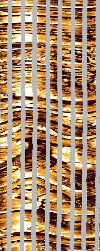
Bowland Shale Reservoir Intervals               43

                                                                                                                                                             Downloaded from https://academic.oup.com/gji/article/228/1/39/6355446 by guest on 08 October 2021

Figure 2. Wireline log character at PH-1. The primary shale gas target is the Upper and Lower Bowland Shales at the base of the well. The overburden
consists of a full Millstone Grit sequence and a thin, incomplete, Lower Coal Measures. A significant unconformity separates the Lower Coal Measures from
Permo-Triassic Manchester Marl, Sherwood Sandstone and Mercia Mudstone (not logged). MD, Measured Depth; GR, Gamma Ray; RHOB, Bulk Density;
NPOR, Neutron Porosity; DTC, Compressional Slowness; DDLL, Deep Laterolog Resistivity; GRUR, Uranium Concentration from Spectral Gamma Ray;
DTS-FAST, Fast Shear Wave Slowness; DTS-SLOW, Slow Shear Slowness (Contains OGA Well Log           C Data accessed and published with permission of BGS).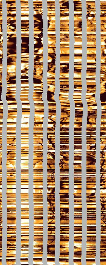
44      I. Anderson et al.

                                                                                   (b)

                                                                                                                                                                     Downloaded from https://academic.oup.com/gji/article/228/1/39/6355446 by guest on 08 October 2021
                                                                                   (c)

      (a)

                                                                                           (d)

Figure 3. A collection of images illustrating the presence of natural fractures within the Bowland Shale [after Fauchille et al. (2017) and Clarke et al. (2018)].
A full caption is provided in the inset text box (Contains OGA Well Log   C Data accessed and published with permission of BGS).

   The upscaling of such studies to wireline log and/or seismic data                Effective medium models
also poses an additional challenge. Accurately measuring the degree
                                                                                    In this work, a rock physics models are built to characterize the
of VTI anisotropy and gaining an understanding of the inherent
                                                                                    elastic properties of the Bowland Shale, the foundations of which are
causes of it can better inform modelling work at the larger scale
                                                                                    built on effective medium theory (EMT). EMT allows for the mixing
(i.e. wireline log or seismic scale), but upscaling these effects can
                                                                                    of multiple constituents (i.e. minerals, pores or fluids) considering
be troublesome. Laboratory measurements can only be performed
                                                                                    their volume fraction, individual elastic properties and (generalized)
on either intact samples or samples with healed (i.e. mineralized)
                                                                                    shape. The background theory to many of the effective medium
fractures that may not be representative of the fractured rocks at
                                                                                    models used in this work can be found in Mavko et al. (2009) and
depth. Furthermore, the relative contributions of microscale features
                                                                                    recent reviews such as Zhang (2017), Zhang et al. (2017), Guo &
that affect VTI anisotropy to anisotropy measurements acquired at
                                                                                    Liu (2018) and Dvorkin et al. (2021). We outline some of the theory
the broader scale (e.g. shear wave splitting) is uncertain.
                                                                                    pertinent to this work within the Appendix.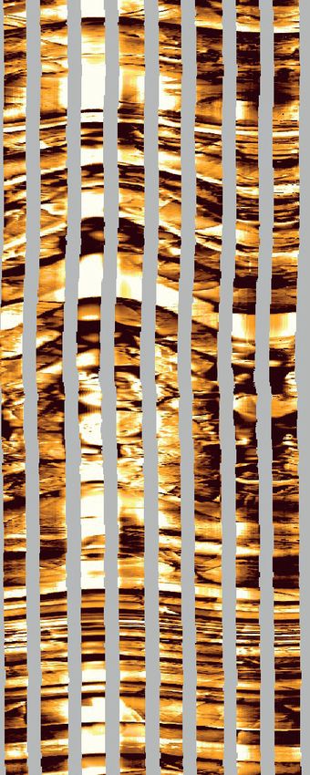
Bowland Shale Reservoir Intervals                 45

    (a)                                                (b)                                                (c)

                                                                                                                                                                 Downloaded from https://academic.oup.com/gji/article/228/1/39/6355446 by guest on 08 October 2021
Figure 4. Dynamic Compact Micro-Imager (CMI-Dynamic) log and shear anisotropy logs plotted for three depth intervals within the Bowland Shale at PH-1.
Shear anisotropy appears to be greatly influenced by fractures. In the case of the middle and right plots, subvertical fractures (shown as sinusoidal shapes)
appear to be causing the anisotropy, whereas, on the left plot, vertical, induced fractures appear to be the main cause (Contains OGA Well Log
                                                                                                                                               C Data accessed

and published with permission of BGS).

METHODS                                                                           quantitative lithology measurements derived from direct measure-
                                                                                  ments of elemental yields within the formation (e.g. Elemental Cap-
Rock properties                                                                   ture Spectroscopy (Herron & Herron 1996) but may not be included
                                                                                  as part of a standard wireline logging suite, and was not run at PH-1
Full characterization of a shale gas reservoir requires the integration
                                                                                  (Table 1). Determining quantitative lithology using traditional log-
of various scales of data and the degree of uncertainty associated
                                                                                  ging suites is achieved more often using a multimineral inversion
with these data sets increases with increasing scale of coverage.
                                                                                  approach, such as that followed by Schlumberger’s Elemental Log
Core studies provide accurate quantification of mineralogy, total or-
                                                                                  Analysis program (ELAN, Quirein et al. 1986).
ganic content (TOC), porosity, permeability and saturation however
                                                                                     The ELAN program is packaged within Schlumberger’s Techlog
sample sizes are often limited. Wireline logging provides continu-
                                                                                  petrophysical software and was accessed for this work. Analysis of
ous measurements of various physical properties every 0.1524 m
                                                                                  wireline logs is the inverse of the forward problem stated as (Quirein
(though actual bed resolution varies by tool type) however these
                                                                                  et al. 1986):
often require transformation into relevant rock properties. Seismic
data provides 3-D measurements of reflectivity at 10s-m resolution                t = Rv,                                                                 (2)
however well logs are required to produce a meaningful inversion
and generate predictions of rock or reservoir properties. The first               where t is the tool vector consisting of the log readings at a cer-
step in performing a petrophysical analysis of the RQ at PH-1 and                 tain depth, R is the response matrix of constant parameters and v
generating data for the rock physics model is to calculate continuous             is the volume component vector. The aim of multimineral inver-
logs of mineralogy, TOC, porosity, and saturation. Throughout the                 sion is determining v, given a series of tool measurements, t and
analysis, attempts were made to honour any information from PH-1                  a user-defined response matrix, R. The inversion approach (Mayer
core reports, including mineralogical data from XRD tests, porosity,              & Sibbit 1980) involves iteratively solving the above forward prob-
permeability and saturation data from Mercury immersion and He-                   lem, minimizing the error between reconstructed tool response and
lium pycnometry tests and TOC data from Source Rock Analyzer                      actual tool response (Quirein et al. 1986). If a fixed response matrix
(SRA) pyrolysis (Table 2).                                                        is assumed, the volume of each component can be inverted for in
                                                                                  this approach.
                                                                                     Prior knowledge of the typical mineralogical assemblages within
                                                                                  the formation is required, as should an understanding of the appro-
Mineralogy logs—elemental log analysis (ELAN)                                     priate logs to be used as input. The program can invert for the same
                                                                                  number of mineralogical components as input log measurements
Determining complex mineralogy from wireline logs is a chal-
                                                                                  plus one (Quirein et al. 1986). The tool response for each mineral
lenging task in the shale reservoirs. Spectroscopy logging provides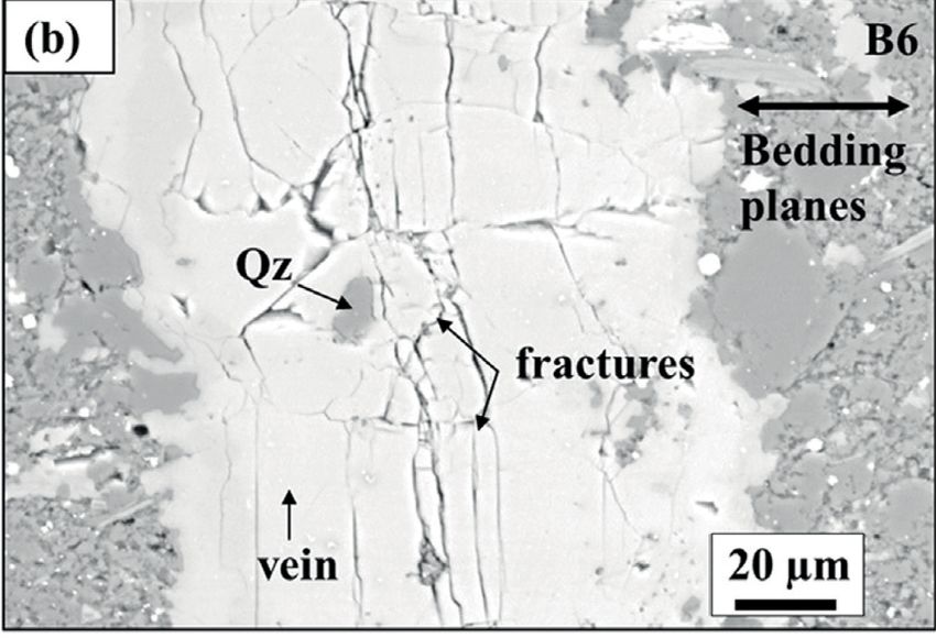
46      I. Anderson et al.

                  Table 3. Default response parameters for the three log inputs to the ELAN model for the three minerals to be inverted.
                  The neutron porosity log is calibrated to limestone, which results in a zero-porosity value for pure limestone and a
                  negative reading for quartz.
                                        Bulk density (g cm–3 )         Neutron porosity (v v–1 )      Compressional slowness (μs ft–1 )
                  Clay                          2.63                             0.37                               55.3
                  Quartz                        2.65                            –0.03                               55.5
                  Carbonate                     2.71                              0                                 47.5

must also be known (e.g. the RHOB log in a 100 per cent quartz                  density of kerogen. The density of kerogen will vary with maturity,
formation will read 2.65 g cm–3 ). In practice, response parameters             which itself varies with depth of the Bowland Shale in the PH-1
would be extracted from a database using adjacent wells and/or lab-             well. Clarke et al. (2018) demonstrate vitrinite reflectance (Ro ) to
oratory studies. While ideally, a bespoke set of response parameters            vary between 1.5 and 2.25 (corresponding to the early-wet gas to
would be determined for the Bowland Shale using wireline logs                   early-dry gas window). For this maturity range, kerogen densities
(including elemental logs ‘Elemental Capture Spectroscopy’) and                 of around 1.4–1.5 g cm–3 are reasonable (Alfred & Vernik 2013),
core analysis from multiple wells, for this work, as only one well              and in our calculations we set the parameter to 1.4 g cm–3 . Kerogen

                                                                                                                                                           Downloaded from https://academic.oup.com/gji/article/228/1/39/6355446 by guest on 08 October 2021
was available, with some limited core data, the response parameters             concentration is plotted alongside measurements from core data
were kept at program defaults (Schlumberger 2019, Table 3).                     (calculated from TOC using the same approach) for comparison in
   Three wireline logs that are strongly influenced by lithology were           Fig. 5 (track 8).
selected for use in the ELAN model: NPOR, RHOB and DTC.
Throughout the inversion, reconstructed tool measurements were
compared with actual measurements to ensure errors were kept to a               Water saturation
minimum. Log outputs were also compared with core XRD (Table 2)                 Estimation of water saturation is a challenging task in shales with
information to ensure reasonable results (Fig. 5).                              many of the well-adopted methods developed on clean or shaly
                                                                                reservoir sands. While this thesis does not address the calculation
                                                                                of water saturation in detail, a method considered most applica-
TOC and kerogen concentration
                                                                                ble in shaly settings [the Indonesia method proposed by Poupon
Several approaches exist to determining TOC and Kerogen concen-                 & Leveaux (1971)] was picked to determine an approximation of
trations from wireline logs. The most popular methods include de-               saturation. The equation uses formation resistivity, the volume of
veloping empirical correlations with laboratory TOC measurements                shale/clay and porosity as follows:
(Fertl & Chilingar 1988) or the analysis of the separation between                     ⎧                            ⎫(2/n)
porosity-based and fluid-based logs (logR, Passey et al. 1990).                       ⎪
                                                                                       ⎪                   1        ⎪
                                                                                                                    ⎪
                                                                                       ⎪
                                                                                       ⎨                            ⎪
                                                                                                                    ⎬
As this latter approach is largely based on the elevated resistivity                                     Rt
                                                                                SW =                                      ,                    (5)
response due to liquid hydrocarbons it is not always transferable to                   ⎪
                                                                                       ⎪   Vsh (1−0.5Vsh )
                                                                                                                φ ⎪
                                                                                                                 m
                                                                                                                    ⎪
                                                                                       ⎪
                                                                                       ⎩      √              +      ⎪
                                                                                                                    ⎭
overmature gas shales and therefore is not followed in this work.                                Rsh           a Rw
   Of the different correlations proposed between wireline logs and
TOC, one of the strongest involves Uranium concentration (GRUR;                 where Vsh is shale volume (taken as clay volume from the ELAN
Fig. 2). As authigenic Uranium precipitates at the sediment-water in-           model), ϕ is porosity and Rt is formation resistivity. Picking appro-
terface under anoxic conditions and accumulates along with organic              priate values for tortuosity, cementation, and saturation exponents
matter, Uranium and TOC have been shown to strongly correlate                   (a, m and n) can be a challenge. Values of 1, 2 and 2, are widely used
(Supernaw et al. 1978; Lüning & Kolonic 2003). In the Bowland                  in the conventional setting, however, these are appropriate only for
Shale, we observe high Uranium concentrations, particularly within              clay-poor rocks with well-connected pores. Some authors have sug-
the UBS, up to 10 ppm and corresponding to total GR readings of                 gested that the cementation exponent is the fundamental parameter
∼200 API (Fig. 2). Using this log data and TOC measurements                     that should be adjusted in the case of shales, which led Maleki-
available from core data (Table 2), a linear correlation is estab-              mostaghim et al. (2019) to conduct a laboratory study to determine
lished:                                                                         a reasonable value for shale. We use their determined value of 1.6 in
                                                                                our calculations. The resistivity of water (Rw ) and of shale (Rsh ) are
T OC = 0.015 × Ur − 0.02,                                             (3)       fixed at 0.03 and 5, respectively. This method provides a reasonable
where TOC is measured as a fraction and Ur is in ppm. TOC was                   fit to the lower values of core-measured water saturation (Fig. 5;
then converted to Kerogen using the approach of Herron & Le                     track 9) but does not accurately capture the higher core-derived
Tendre (1990) and Vernik & Nur (1992):                                          values.

       C × TOC × ρb
VK =                ,                                                 (4)
            ρk                                                                  Permeability
where C is a TOC to Kerogen conversion factor. While the maturity               The relationship of permeability and porosity is complex, and reser-
of the Bowland Shale at PH-1 makes it difficult to infer original               voir zones of similar porosity can exhibit markedly different per-
kerogen type (Clarke et al. 2018), it is generally believed to consist          meabilities. This has led some authors to recognize the presence of
of a mixture of Types II (marine) and III (terrestrial) (Andrews 2013;          ‘flow units’ using cross-plots of core-derived porosity and perme-
Slowakiewicz et al. 2015; Hennissen et al. 2017; Clarke et al. 2018).           ability data (Corbett & Potter 2004; Aguilera 2014). In the absence
For these kerogen types, situated in the gas window, Tissot & Welte             of substantial core test data, permeability models become more un-
(1978) suggest a conversion factor around 1.2 is suitable, which we             certain, though fitting an exponential trend is often considered a
follow in our calculations. ρ b is the RHOB log reading and ρ k is the          reasonable approximation (Halliburton 2019).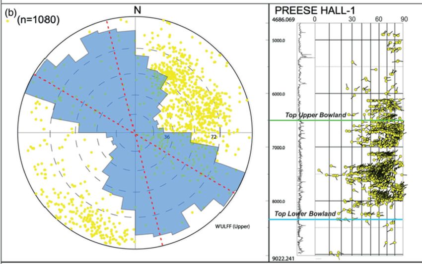
Bowland Shale Reservoir Intervals                 47

                                                                                                                                                                  Downloaded from https://academic.oup.com/gji/article/228/1/39/6355446 by guest on 08 October 2021

Figure 5. Log display illustrating the input logs to the rock physics model and core analysis data. Mineralogy and porosity (tracks 3–5 and 7) are derived from
the ELAN inversion model. Kerogen concentration (track 8) is derived from a linear regression model fitted to GRUR and core TOC. Water saturation (track
9) is estimated using the Indonesia method. Sw, Water Saturation (Contains OGA Well Log      C Data accessed and published with permission of BGS).
48 I. Anderson et al.
from average values obtained from core XRD data. Likewise, car-
bonate is modelled as a calcite/dolomite mixture. The proportions
of each mineral within its mixed group (i.e. clay and carbonate) do
not change within the model.
(2) The pore system within the Bowland Shale is mainly within
or associated with organic matter (Ma et al. 2016). To represent
this, a kerogen/gas mixture is created using the approach followed
by Carcione (2000) whereby the mixture consists of hydrocarbon
bubbles embedded within a kerogen matrix. Carcione (2000) first
used Wood (1955)’s equation to create a water/oil mixture, which we
follow but consider gas rather than oil. We take the water saturation
log as the water fraction and assume the hydrocarbon saturation
to be composed entirely of gas. Secondly, Carcione (2000) used
Kuster & Toksöz (1974)’s model to embed spherical fluid (water
and gas) pores into the kerogen matrix. This approach was also
followed by Guo et al. (2013) in their model for the Barnett Shale.
Downloaded from https://academic.oup.com/gji/article/228/1/39/6355446 by guest on 08 October 2021
Following Guo et al. (2013), we assume that the percentage of the
total porosity allocated to kerogen is fixed at 20 per cent throughout
Figure 6. Total porosity versus permeability cross-plot using data from
core analysis at PH-1. The exponential regression was used to estimate a
the shale. This will likely vary with maturity, but given their work
permeability log from ELAN porosity (Contains OGA Well Log C Data focused on the Barnett Shale, we consider it a reasonable general
accessed and published with permission of BGS). value for gas mature shales. The remaining 80 per cent of total
porosity is then added as isolated, fluid-filled (also water and gas)
Some limited effective porosity and matrix permeability core pores in step 3.
test results are available for PH-1 (Table 2), and while they were (3) Berryman (1980)’s SCA model is then used to create a mix-
not sufficient in number to carry out a detailed rock typing exercise, ture of the solid minerals (quartz, carbonate and clay), porous kero-
they did allow the building of an approximate permeability model gen and remaining isolated pores. The fractions of each constituent
(Fig. 6). Note that the core-derived matrix permeability values are are taken from the appropriate input log. We consider quartz and
very low, ranging from 2 to 50 nD. This exponential function was carbonate as spherical (aspect ratio of 1), and the kerogen, clays and
used to estimate a continuous permeability from the ELAN porosity. pores as ellipsoidal in shape (aspect ratio of 0.1).
The permeability curve was used in the final classification but not
in the rock physics model itself.
Anisotropic model
Rock physics model Anisotropy is considered within the rock physics model by adding
vertical, aligned, water-filled cracks into the rock to simulate the ef-
In building a rock physics model for the Bowland Shale, two broad
fect of natural, sub-vertical fractures within the formation. The shear
aims were pursued. First, to account for the lithological heterogene-
wave splitting log forms the basis for the inversion, with the aim be-
ity described in previous sections, while honouring observations
ing to quantify the degree of vertical/sub-vertical fractures observed
made regarding the fabric of the shale, and to investigate its impact
on the micro-imagery log data by calibrating an anisotropic rock
on elastic properties. Secondly, given the observations of natural
physics model to shear anisotropy observed from the cross-dipole
fractures within the shale and the effects on shear wave anisotropy,
sonic logging data. However, as was highlighted previously, there is
to invert the Hudson crack density parameter (a metric that can be
evidence from the micro-imagery log that zones of drilling-induced
seen as a proxy for the density of natural fractures) and quantify the
tensile fractures are also contributing to the shear wave splitting
degree of anisotropy associated with it.
behaviour within the shale. Attempt was not made to decouple the
effects of natural and drilling-induced fractures on the shear wave
Isotropic model anisotropy log, though effective medium techniques have proven
efficient in distinguishing the two phenomena (Prioul et al. 2007).
A rock physics model essentially seeks to transform rock properties Instead, a prominent zone of intense drilling-induced fractures be-
(such as lithology, porosity, and fluid saturation) to elastic properties tween 2127 and 2170 m (measured depth) was eliminated entirely
(Grana 2014). In shales, the task is challenging due to the presence as to avoid it dominating the inversion calculations. Fig. 4 (left)
of complex microstructural fabrics, mineralogical variability, and showed the micro-imagery log response and associate shear wave
the presence of microcracks and fractures which all, in turn, sig- anisotropy character for a subsection of this zone.
nificantly affect the elastic properties of the rock. Therefore, rock To ensure that the inverted crack porosity and non-crack porosity
physics models for shales usually involve multiple modelling steps (from the ELAN model) do not exceed the total porosity of the rock,
and utilize several numerical algorithms to best approximate the our inversion scheme begins with initial estimates of crack density
rock’s complex physical properties and account for anisotropy. The (per unit volume). We assume that crack density (ρ c ) is linearly
rock physics model implemented in this work sought to encompass related to shear wave anisotropy (γ ) as:
the effects of porosity, kerogen and mineralogy on elastic properties
and involves several steps outlined as follows: ρc = k × γ , (6)
(1) Elastic constants for mixed clay and mixed carbonate are cal- where k is a factor that converts shear wave anisotropy (expressed
culated using the Hashin–Strikman average. Clay is modelled as an as a per cent) to crack density (expressed as a fraction). According
illite/kaolinite mixture with the proportion of each mineral taken to Kachanov & Mishakin (2019, their eq. 11), crack porosity (ϕ c )Bowland Shale Reservoir Intervals 49
can then be estimated from crack density as: Validation of isotropic model
To assess the durability of the isotropic rock physics model, com-
ϕc = α × ρ c , (7)
pressional (P-wave) velocity (VP ) and shear (S-wave) velocity (VS )
where α is the aspect ratio of the cracks. curves were modelled for a section near the base of the UBS and
Once crack porosity is estimated, an isotropic rock is then con- checked against the actual VP and VS logs (Fig. 9). Both modelled
structed according to the method outlined in the previous section. curves show a good match with the actual data. The VP model dis-
The porosity added in the isotropic model is adjusted by subtract- plays the strongest match with a correlation coefficient (R) of 0.89
ing the crack porosity from the total porosity to ensure that when for this interval, an intercept close to zero and a gradient near one
cracks are added in subsequent modelling, the total porosity is not (Fig. 9c). A small number of low VP values are not captured in the
exceeded. Following this, the Hudson model is used to add vertical model (e.g. at 2300 m, also evident as datapoints positioned far
cracks, with the shape of the cracks fixed as very narrow ellipsoids above the linear regression trend), but as these are few, the overall
(aspect ratio of 0.1). performance of the VP model was considered adequate.
The Hudson model provides an output of the full anisotropic The VS model shows a slightly weaker match, with an R-value
stiffness tensor for that crack density. We use this to calculate of 0.77 for this interval. A systematic, slight overprediction is ob-
equivalent slowness logs by assuming transverse isotropy with a served as evidenced by the linear regression fit positioning further
Downloaded from https://academic.oup.com/gji/article/228/1/39/6355446 by guest on 08 October 2021
horizontal plane of symmetry (HTI) whereby the fast shear wave up the y-axis (‘Modelled VS ’) than the Y = X trend in Fig. 9(d).
(DTSfast ) propagates normal to bedding and the slow shear wave The poorer correlation could be partially explained by differences
(DTSslow ) propagates parallel to bedding. Thus, the modelled shear between the log types. The shear velocity log is derived from the
wave anisotropy becomes: cross-dipole sonic tool which has a typical bed resolution of ∼1.4 m.
However, the input logs to the ELAN model form part of a suite
(DT Sslow − DT Sfast ) of tools (termed quad combo) most of which can achieve bed reso-
γ = × 100. (8) lutions ∼30 cm. While all wireline logs are presented with a con-
DT Sfast
sistent 0.1524 m sampling rate, the bed resolution (i.e. the thinnest
Therefore, a log of modelled shear wave anisotropy for a given unit that can be identified) achieved by each log is variable. Cou-
k (eq. 8) is determined. The quality of fit between this modelled pling these differences in resolution with uncertainties regarding
curve and the actual anisotropy log is assessed by calculating the the depth-matching of separate logging runs could partly explain
mean squared error (MSE), and the process is repeated for different the poorer relationship observed in the VS model. Nevertheless, in
values of k (ranging from 0.002 and 0.011). Using this approach, the the absence of additional information to assess this, the correla-
resulting MSE ranged between 6.2 and 0.03 (Fig. 7a), with the latter tions were considered reasonable, and sufficient for use in the rock
corresponding to a k of 0.08. At k values above this, the modelled physics templates and the subsequent inversion.
overpredicts the degree of anisotropy and at k values below this, it
underpredicts (Fig. 7b).
Rock physics templates
Following assessment of rock physics model’s performance, cross-
plots were produced to compare the measured elastic properties
from wireline logs at PH-1 with the predicted elastic properties
R E S U LT S
from the rock physics model and to provide some insight into the
link between the Bowland Shale’s rock and reservoir properties and
Reservoir properties
geophysical data. Fig. 10 presents these cross-plots with a focus
The results of the multimineral inversion using ELAN, reveal that on the lithological character of the shale. The wireline log data is
quartz is the dominant mineral within the Bowland Shale (Fig. 8). plotted as scattered data coloured by lithology classification (fur-
Most of the shale contains quartz concentrations between 50 and ther outlined in Fig. 11). The rock physics model is presented as
80 per cent with means of 59.4 and 52.0 per cent for the UBS and a pseudo-ternary diagram in rock physics space. A full range of
LBS, respectively. Clay and carbonate concentrations are lower, with clay, carbonate and quartz concentrations are iterated over; how-
means around 24.5 and 20 per cent, respectively though clay con- ever, kerogen concentration and water saturation are fixed at their
centration displays a normal distribution around the mean, whereas median values (3.8 and 9.8 per cent, respectively). Further argument
the carbonate distribution is skewed towards the lower values. The around the median values is provided in the Discussion section. Two
mean carbonate content in the LBS is greater (25.5 per cent) than in models of fixed porosity are considered; a zero-porosity model rep-
the UBS (18.0 per cent), and while carbonate content is generally resented as black lines with colour-fill, and a 10 per cent porosity
low, there are some intervals with very high concentrations up to model represented as grey lines with no fill.
80–90 per cent. The colour-fill used in both the scattered data and the model is
TOC content is largely between 1 and 4 per cent and is noticeably designed to highlight certain lithologies using a simplified version
higher in the UBS (2.7 per cent mean) than the LBS (1.5 per cent of the sCore scheme for shale lithology classification (Gamero-Diaz
mean). Total porosity is mainly less than 6 per cent with means of et al. 2012). Fig. 11 demonstrates the relationship between mineral
4.2 and 3.8 per cent for the UBS and LBS, respectively. Lastly, our content and lithology classification with the data points plotted from
modelled water saturation is almost exclusively less than 30 per cent, the ELAN model. The number of lithological classifications is fewer
which with means of 11.2 and 10.3 per cent for the UBS and LBS, than that used in Gamero-Diaz et al. (2012) and the colour scheme
respectively. These values appear quite low and fail to capture the adjusted to allow greater contrast between the lithologies and assist
higher water saturation core measurements as illustrated on Fig. 5 with visualization of the cross-plots. Also shown beneath the model
(track 9). The values of 100 per cent in this instance correspond to and data points are general zones of brittle and ductile rocks (after
zero porosity sections of the shale. Perez Altamar & Marfurt 2014). Brittleness index was calculated for50 I. Anderson et al.
(a)
Downloaded from https://academic.oup.com/gji/article/228/1/39/6355446 by guest on 08 October 2021
(b)
Figure 7. Plots illustrating the fit of the inversion technique to the shear wave anisotropy log. Upper: plot of Mean Squared Error (MSE) with different k (ratio
of crack density to shear wave anisotropy) values, showing that the lowest MSE corresponds to a k of 0.008. Lower: Plot of predicted versus actual shear wave
anisotropy for the entire Bowland Shale interval with the points coloured by k value. A k value of 0.008 produces modelled values that lie close to the y = x
line (Contains OGA Well Log C Data accessed and published with permission of BGS).
each data point using the Rickman et al. (2008) method where Emin low strength; less stress is required to induce strain in the rock),
and ν max (ductile rock) were set to 26.1 GPa and 0.40, respectively highest ν values (i.e. low strength; high transverse strain upon axial
and Emax and ν min (brittle rock) were set to 67.6 GPa and 0.08, loading) and lowest AI values (i.e. low resistance to a propagating
respectively. The results of this calculation were used to interpret compressional wave). VP to VS ratio alone does not appear a useful
zones of brittle and ductile zones elastic properties on each cross- indicator for this lithology, as it spans a range of values between 1.7
plot. and 2.1 (Fig. 10c) and displaying some overlap with the carbonate
In each figure, four rock physics templates are shown: (1) Lamé regions of the shale.
incompressibility multiplied with bulk density (λρ) versus Lamé The predominant lithology is siliceous mudstone which displays
rigidity multiplied by bulk density (μρ) (Goodway et al. 1997, greater rigidity (μρ > 40 GPa g cm–3 ) than the argillaceous mud-
2010), (2) Acoustic Impedance (AI) versus VP to VS ratio, (3) VP stone and equal, to slightly lower incompressibility (λρ, Fig. 10a).
versus VS and (4) Poisson’s ratio (ν) versus Young’s modulus (E). It exhibits the lowest VP to VS ratio (Bowland Shale Reservoir Intervals 51
Downloaded from https://academic.oup.com/gji/article/228/1/39/6355446 by guest on 08 October 2021
Figure 8. Histograms of rock and reservoir properties calculated for the Bowland Shale. The histograms are separated into the UBS (red) and LBS (blue). For
each histogram, the mean and standard deviation are annotated (Contains OGA Well Log C Data accessed and published with permission of BGS).
(up to 110 GPa g cm–3 ), accompanied by a subtle increase in μρ Fluctuations in these parameters will cause changes in elastic prop-
(Fig. 10a). An increase is observed for both AI (from 14 to 16 km s–1 erties and affect the shape of the triangular mesh on the charts that
· g cm–3 ) and VP to VS ratio (from 1.7 to 1.9, Fig. 10b), though as represents the rock physics model. However, when producing such
previously discussed, this trend in VP to VS ratio is also observed for a generalized template this is difficult to avoid. Producing multiple
the argillaceous mudstone. It is also characterized by high ν and E charts with multiple distributions of these fixed parameters is pos-
(Fig. 10d). This high Poisson’s ratio translates to a slight decrease sible, but in doing so, the predictive power of them is lost and it
in brittleness, relative to the siliceous mudstone lithology. becomes harder to interpret the results in a general sense.
We also observe errors between the template lithology and lithol- On the whole, the results suggest that lithology has an acute
ogy of the data points (for example, some mixed mudstone data control on the elastic properties of the shale. The shale exhibits
points fall within the calcareous mudstone template zone (Fig. 10a)). predominantly brittle characteristics as evidenced by the relation-
This could be explained by the fact that porosity, kerogen content, ship between the well log data points and the generalized brittleness
water saturation and some textural parameters (e.g. aspect ratios classification. The most brittle sections of the shale appear to lie
of minerals) are all fixed in the generation of the model template. within the mixed mudstone lithology. As quartz content is often52 I. Anderson et al.
(Fig. 12). On the basis of the above observations, given this interval
has moderate-high porosity and relatively low carbonate concentra-
(a) (b) tions, we would expect this interval to display low-moderate crack
densities, however this cannot be confidently tested.
Rock physics templates were again produced but in this instance
with data points coloured by inverted crack density (Fig. 13). The
relationship between elastic properties and crack density is not an
obvious one, but they do clearly show a preference for plotting
within the brittle sections of the cross-plot (see Fig. 10 for the full
brittleness template). Areas of high crack density (yellows, greens)
correlate to high μρ (12 km s–1 · g cm–3 , Fig. 13b) and Young’s modulus (>50 GPa,
Fig. 13d) but cover a range of VP to VS ratio (Fig. 13b) and Pois-
Downloaded from https://academic.oup.com/gji/article/228/1/39/6355446 by guest on 08 October 2021
son’s ratio (Fig. 13d). We previously described how high μρ, high
Young’s modulus and low AI correspond to both siliceous and cal-
careous mudstones, and that the clearest indicator of carbonate is
high λρ. Taking this into account when interpreting Fig. 13, and
in alignment with the observations of Fig. 12, it would appear that
while natural fractures do show a preference for clay-poor zones,
there is little clarity provided in these plots as to whether they are
forming preferentially in siliceous or calcareous beds.
(c) (d) Reservoir quality evaluation
To evaluate the presence of high RQ intervals within the Bowland
Shale section at PH-1, five parameters are used: clay concentration,
porosity, permeability, TOC content and water saturation (Table 4).
Figure 9. Plots of VP and VS compared to modelled VP and VS data (a, b) The zones that pass all these cut-offs are shown in log view (Fig. 14)
and associated cross-plots (c, d) (Contains OGA Well Log
C Data accessed and rock physics space (Fig. 15). The rock physics model is shown
and published with permission of BGS). in the same manner as Figs 10 and 13 but with data points coloured
where a RQ interval exists. To better identify the portion of the
considered the main contributor to shale brittleness, this is an un- plots where the density of RQ intervals is highest, a bivariate kernel
usual observation. However, these siliceous mudstone units also density estimation is used, with shading strongest where density is
display moderate porosity, which would serve to reduce the rigid- greatest.
ity of the rock. Brittleness appears to reach a maximum within Clay concentration is a key factor in the evaluation of a shale
low porosity, moderately calcareous mudstones, but then falls with gas reservoir. The best production within the Barnett Shale comes
further carbonate content. Carbonate minerals such as calcite and from zones with 27 per cent clay (Bowker 2003), and 50 per cent
dolomite exhibit greater Poisson’s ratio (∼0.30) than quartz (0.08, has been suggested as the maximum clay concentration for which a
Mavko et al. 2009), which may explain the reduction in brittleness shale could be hydraulically fractured (Bowker 2007). Based on this,
observed for carbonate-rich intervals when Rickman et al. (2008)’s a 50 per cent maximum cut-off was taken for clay concentration.
approach is used. This behaviour was also observed by Perez Alta- As the clay concentration in the majority of the Bowland Shale
mar & Marfurt (2014) in their Barnett Shale study and does suggest is beneath this cut-off (Fig. 14, track 3), this had minimal effect
that interpreting siliceous from carbonate-rich intervals using elas- in reducing the prospective interval besides eliminating a clay-rich
tic property cross-plots should ideally be checked against available interval at the very top of the UBS and three clay-rich intervals in
mineralogical data. the LBS.
Shale porosity is an important parameter in assessing the storage
potential of the formation. Jarvie (2012) suggests that porosity for
Crack density inversion
an effective shale gas reservoir should be between 4 and 7 per cent.
The inverted crack density is predominantly below 0.04 but does Taking 4 per cent as a minimum cut-off on its own has a marked
exceed 0.06 in some intervals (e.g. 2200, 2260 and 2285 m, Fig. 12). effect on reducing the prospective interval as it is very close to the
It appears to show an inverse relationship with total porosity and median value (3.8 per cent) thus eliminating near half of the shale.
clay fraction. In some intervals (e.g. those quoted above), high crack Notably, this eliminates the Pendleside Sandstone Member in the
density appears to be associated with high carbonate fractions, how- LBS [e.g. Fig. 14 (track 4) between 2500 and 2600 m].
ever this relationship is less apparent at greater depths (e.g. 2540 m) TOC is a metric of the potential for a shale to generate hydrocar-
where high carbonate fractions correspond to moderate crack den- bons which is usually used in combination with Hydrogen Index, S2
sity. On this plot, the zone of intense drilling-induced fractures (generation potential) and other geochemical parameters to assess
(DIFs) that was omitted from the inversion is highlighted in red source rock quality. It is purely a measure of the present-day organicBowland Shale Reservoir Intervals 53
Downloaded from https://academic.oup.com/gji/article/228/1/39/6355446 by guest on 08 October 2021
(a) (b)
(c) (d)
Figure 10. λρ versus μρ (a), AI versus VP /VS (b), VP versus VS (c) and ν versus E (d) cross-plots for the Bowland Shale. The scattered data is wireline log
elastic properties from PH-1 with samples every 0.1524 m, coloured by the lithology type determined from the ELAN model. The triangular mesh represents
the rock physics model iterating over concentrations of clay, quartz and carbonate with fixed kerogen concentration and water saturation. Porosity is fixed at 0
per cent (black lines with a colour fill) and 10 per cent (grey lines, no fill). Also shown is a simplified brittleness classification after Perez Altamar & Marfurt
(2014). The lithology colour scheme is shown in Fig. 11 (Contains OGA Well Log C Data accessed and published with permission of BGS).
richness of the formation which will have been reduced since de- respectively. The final cut-offs are defined in Table 4 and Fig. 14. A
position due to burial, maturation and expulsion of hydrocarbons. total rock thickness of 125 m is found pass all five of these criteria
Jarvie (2012) suggests that 1 per cent present-day TOC is sufficient (Fig. 14, track 9). We term this as RQ intervals, for future discus-
to be considered a shale gas reservoir. We take a slightly conserva- sion. While RQ intervals are observed across the entire Bowland
tive cut-off similar to Andrews (2013) of 2 per cent which is very Shale interval, they are predominantly found (92 per cent of the
near the median calculated TOC for the Bowland Shale interval (1.9 total thickness) within the UBS.
per cent). The λρ versus μρ plot reveals a well-defined zone in which RQ
The remaining cut-offs were selected by taking the median value intervals are clustered (Fig. 15a). The highest densities plot between
within the logged section. Minimum and maximum cut-offs were 30 and 50 GPa · g cm–3 λρ and 50–60 GPa · g cm–3 μρ. In the
selected in this manner for permeability and water saturation, remaining plots, the RQ interval is slightly less defined. On the AIYou can also read