Unemployment Effects of Stay-at-Home Orders: Evidence from High Frequency Claims Data - Institute for ...
←
→
Page content transcription
If your browser does not render page correctly, please read the page content below

IRLE WORKING PAPER
                                                                                #101-20
                                                                               July 2020

Unemployment Effects of Stay-at-Home Orders:
Evidence from High Frequency Claims Data

ChaeWon Baek, Peter B. McCrory, Todd Messer, and Preston Mui

Cite as: ChaeWon Baek, Peter B. McCrory, Todd Messer, and Preston Mui. (2020). “Unemployment Effects of
Stay-at-Home Orders: Evidence from High Frequency Claims Data”. IRLE Working Paper No. 101-20.
http://irle.berkeley.edu/files/2020/07/Unemployment-Effects-of-Stay-at-Home-Orders.pdf

http://irle.berkeley.edu/working-papers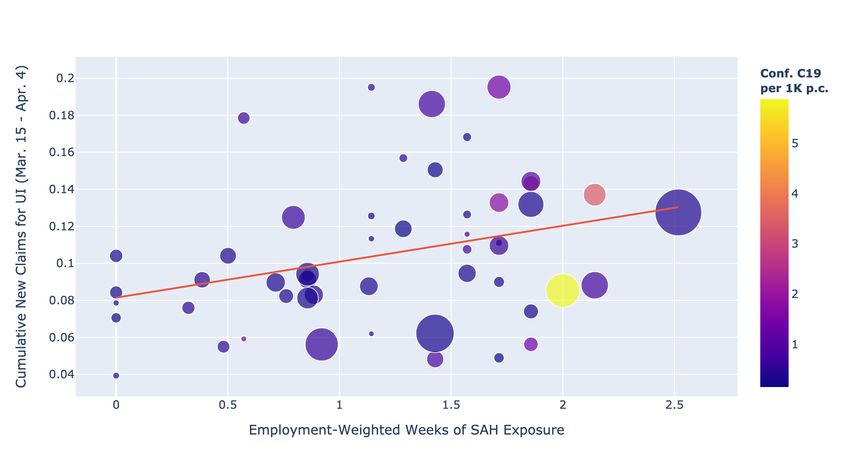
Unemployment Effects of Stay-at-Home Orders:
                Evidence from High Frequency Claims Data

         ChaeWon Baek∗ , Peter B. McCrory∗ , Todd Messer∗ , and Preston Mui∗

                                     First Draft: April 23, 2020
                                     This Draft: July 10, 2020

                                                  Abstract

          Epidemiological models projected that, without effective mitigation strategies, upwards of
      2 million Americans were at risk of death from the COVID-19 pandemic. Heeding the warning,
      in mid-March 2020, state and local officials in the United States began issuing Stay-at-Home
      (SAH) orders, instructing people to remain at home except to do essential tasks or to do work
      deemed essential. By April 4th, 2020, nearly 95% of the U.S. population was under such orders.
      Over the same three week period, initial claims for unemployment spiked to unprecedented
      levels. In this paper, we use the high-frequency, decentralized implementation of SAH orders,
      along with high-frequency unemployment insurance (UI) claims, to disentangle the relative
      effect of SAH orders from the general economic disruption wrought by the pandemic that
      affected all regions similarly. We find that, all else equal, each week of Stay-at-Home exposure
      increased a state’s weekly initial UI claims by 1.9% of its employment level relative to other
      states. Ignoring cross-regional spillovers, a back-of-the-envelope calculation implies that, of the
      17 million UI claims made between March 14 and April 4, only 4 million were attributable to the
      Stay-at-Home orders. This evidence suggests that the direct effect of SAH orders accounted for
      a substantial, but minority share, of the overall initial rise in unemployment claims. We present
      a stylized currency union model to provide conditions under which this estimate represents an
      upper or lower bound for aggregate employment losses attributable to SAH orders.

Keywords: COVID-19, Non-pharmaceutical Interventions, NPIs, Stay-at-Home orders, Unemploy-
ment Effect, UI Claims, Pandemic Curve, Recession Curve.
JEL Codes: C21, C23, E24, E65, H75, I18, J21

   ∗ UC-Berkeley, Department of Economics, Evans Hall, Office 642 (all). Corresponding Author: Peter B. McCrory

(pbmccrory@berkeley.edu). We thank Christina Brown, Bill Dupor, Yuriy Gorodnichenko, Christina Romer, Maxim
Massenkoff, and Benjamin Schoefer for helpful comments and suggestions.

                                                      1
1 Introduction
To limit the spread and severity of the COVID-19 pandemic, officials around the globe turned
to non-pharmaceutical interventions (NPIs), such as shutting down schools, restricting economic
activities to those deemed essential, and requiring people to remain at home whenever possible. In
mid-March 2020, Ferguson et al. (2020) issued a report projecting that, in the absence of the effective
implementation of NPI mitigation strategies, more than 2 million Americans were potentially at
risk of death from the COVID-19 respiratory disease, with many more facing uncertain medical
complications in the near- and long-run.
Soon after, state and local officials in the United States began announcing Stay-at-Home (SAH)
orders, which restricted residents from leaving their homes except for essential activities. The earliest
SAH order was implemented in the Bay Area, California on March 16th, 2020. Three days later,
the governor of California issued a state-wide SAH order. By March 24th, more than 50% of the
U.S. population was under a SAH order (see Figure 1). By April 4th, 95% of the U.S. population
was under a state or local SAH order, likely substantially reducing the supply of and demand for
locally produced goods and services.
At the same time, there was mounting evidence of substantial disruption to labor markets in the
United States. For the week ending March 21st, 2020, the Department of Labor (DOL) reported
that more than 3.3 million individuals filed for unemployment benefits.1 In the subsequent weeks
ending March 28th and April 4th, initial claims for unemployment once again hit unprecedented
highs of more than 6.9 million claims and 6.7 million claims, respectively. Taken together, total
unemployment insurance (UI) claims over this three week period was almost 17 million.
How much of the initially observed increase in UI claims was attributable to the newly implemented
SAH orders? This is not a straightforward question to answer since the increase in unemployment
claims could plausibly be attributed to a multitude of factors other than SAH orders that occurred
at the same time. For example, consumer and business sentiment both declined and economic
uncertainty rose as the pandemic worsened. One stark example of this economic uncertainty was
the swift drop in the value of the S&P 500 stock market index, which lost roughly 30% of its
value between February 20 and March 16, the first day a SAH order was announced in the United
States.
In this paper, we disentangle the local effects of SAH orders from the broader economic disruption
brought on by the COVID-19 pandemic and other factors affecting all states equally. We do so
by providing evidence of a direct causal link between the implementation of SAH orders and the
1 For comparison, in this week one year prior, there were just over 200 thousand initial claims for unemployment
insurance. This was also the first time since the DOL began issuing these reports that the flow into unemployment
insurance exceeded the number of individuals with continuing claims.
2Figure 1: Cumulative Share of Population under Stay-at-Home Order in the U.S.
Sources: Census Bureau, the New York Times; Authors’ Calculations
observed increase in UI claims. To the best of our knowledge, this paper is the first systematic
study of the causal link between SAH orders and UI claims in the United States. This is our main
contribution.
We show that the decentralized implementation of SAH orders across the U.S. induced high-
frequency regional variation as to when and to what degree local economies were subject to such
orders. We leverage the cross-sectional variation in the length of time that states were exposed to
such orders to estimate its effect on UI claims.2,3
We find that an additional week of exposure to SAH orders increased UI claims by approximately
1.9% of a state’s employment level, relative to unexposed states. The effect is precisely estimated
and robust to the inclusion of a battery of controls one might suspect are correlated with both
local labor market disruption and SAH implementation, lending it a causal interpretation. The
set of controls we consider include the severity of the local exposure to the coronavirus pandemic,
state-level political economy factors, and each state’s industry composition.
We use our cross-sectional estimate to calculate the implied aggregate effect of implemented SAH
2 Our variable of interest pertains to the government implementation of SAH orders. Our design does not aim
to capture the effects of, for example, social distancing behaviors that may have taken place in the absence of a
government order.
3 In this paper, we principally focus on UI claims for three reasons: (1) UI claims are among the highest frequency
indicators of real economic activity—especially as it relates to the labor market; (2) These data are consistently
reported at a subnational level; (3) The data are publicly and readily available.
3orders on the number of new unemployment claims. This exercise yields an estimate of approxi-
mately 4 million UI claims attributable to SAH orders through April 4, comprising roughly 24%
of total claims over the time period. We refer to this calculation as the relative-implied aggregate
estimate of employment losses from SAH orders.
We then investigate whether the change in unemployment claims is due to demand or supply side
factors using proxies for local economic activity. Using daily data from Google on local mobility
trends by county, we estimate the on-impact effect of SAH orders on visits to retail and workplace
locations, the former capturing demand shocks and the latter capturing supply shocks. We find
sharp, on-impact, declines in mobility in both the retail and mobility indices, suggesting that SAH
orders worked through both channels. The decline in both mobility indices persists for at least two
and a half weeks, the horizon over which we estimate the event studies.
It is well known that cross-sectional research designs, such as the one employed in our paper, hold
constant general equilibrium effects as well as other aggregate factors. Simply scaling up our cross-
sectional estimate may therefore give a biased impression of the aggregate effect of SAH orders on
UI claims in the United States.
To understand the nature of these general equilibrium forces, we present a simplified currency
union model to provide conditions under which the relative-implied estimate represents an upper
or lower bound on aggregate employment losses. When the SAH shock is viewed primarily as a
technology shock—and in the empirically relevant case—our estimate represents an upper bound
on the aggregate effect. However, when SAH orders are treated as a local demand shock, the
interpretation is a bit more subtle and depends upon the persistence of the shock and degree of price
flexibility. Across all combinations of price rigidity and persistence, we find that our back-of-the-
envelope estimate, at most, understates aggregate employment losses by a factor of approximately
two. With sticky prices and a zero-persistence shock, the relative-implied estimate associated with
the SAH-induced local demand shock understates aggregate employment losses by 12%.
Our evidence from the mobility indices suggests that the SAH shock should be viewed as a com-
bination of both local supply and demand shocks. The model results then imply a (non-binding)
upper bound on UI claims from SAH orders through April 4, 2020 of approximately 8 million. Thus,
relative to the total rise of around 16.5 million, at most around 50% of the total rise in UI claims
over this period can be attributed to SAH orders.
Finally, we document the robustness of our empirical results by considering two alternative research
designs. First, we consider a panel design that allows us to control separately for week fixed effects
and state fixed effects. The inclusion of such fixed effects controls for time-varying aggregate effects
and time-invariant state effects. Second, we estimate county-level specifications which allow us to
control for unobserved state-level factors, such as each state’s ability to respond to and process
4unprecedented numbers of unemployment claims. We find similar results in both cases.
Related Literature
Our paper relates most obviously to the rapidly growing economic literature studying the COVID-
19 pandemic, its economic implications, and the policies used to address the simultaneous public
health and economic crises. The epidemiology literature has focused on the health effects of NPIs.
In a notable study, Hsiang et al. (2020) estimate that, in six major countries, NPI interventions
prevented or delayed over 62 million COVID-19 cases.4 Our focus is, instead, on the macroeconomic
effects of the coronavirus pandemic. Broadly speaking, the macroeconomic literature on COVID-19
has split into two distinct yet highly related strands. Here we provide a representative, albeit not
exhaustive, review.
The first strand of research focuses on the relationship between macroeconomic activity, policy, and
the unfolding pandemic. Gourinchas (2020) and Atkeson (2020) are early summaries of how the
public health crisis and associated policy interventions interact with the economy. Both emphasize
the trade-off between flattening the pandemic curve while steepening the recession curve. Similarly,
Faria–e–Castro (2020) studies the effect of a pandemic-like event in a quantitative DSGE model in
order to assess the economic damage associated with the pandemic along with the fiscal interventions
employed in the U.S. to attempt to flatten the recession curve. Eichenbaum, Rebelo, and Trabandt
(2020) derive an extension of the standard Susceptible-Infected-Recovered (SIR) epidemiological
model to incorporate macroeconomic effects, formalizing the relationship between the flattening
the pandemic curve and amplifying the recession curve. We view our paper as providing causally
identified, empirical support for the claim that flattening the pandemic curve requires steepening
the recession curve.
The second strand of research uses high-frequency data to understand the economic fallout wrought
by the COVID-19 pandemic. Our paper aligns more closely with this strand of the literature. Baker
et al. (2020) show that economic uncertainty measured by stock market volatility, newspaper-based
economic uncertainty, and subjective uncertainty in business expectation surveys rose sharply as the
pandemic worsened. Lewis, Mertens, and Stock (2020) derive a weekly national economic activity
index and show that the COVID-19 outbreak had already had a substantial negative effect on the
United States economy in the early weeks of the crisis. Hassan et al. (2020) use firm earnings calls
to quantify the risks to firms as a result of the COVID-19 crisis. Coibion, Gorodnichenko, and
Weber (2020b) examine how the pandemic affected the labor market in general. Using a repeated
large-scale household survey, they show that by April 6th, 2020, 20 millions jobs were lost and the
labor market participation rate had fallen sharply.
4 The six countries are China, South Korea, Italy, Iran, France, and the United States.
5Our paper also relates to empirical work studying the effect of lockdown policies more specifically.
For example, Hartl, Wälde, and Weber (2020) study the effect of lockdowns in Germany on the
spread of the COVID-19. In contrast to these papers, we use geographic variation to understand
the effect of COVID-19 on economic activity. In that respect, our paper can be thought of a
high frequency version of Correia et al. (2020), who find that over the long term, NPI policies
implemented in response to the 1918 Influenza Pandemic ultimately resulted in faster growth during
the recovery following the pandemic.
Other papers employing geographic variation in NPI implementation to understand their contribu-
tion to the economic fallout associated with COVID-19 pandemic include the following: Kong and
Prinz (2020) use high-frequency Google search data as a proxy for UI claim activity to study the
labor market effects of various NPIs; Coibion, Gorodnichenko, and Weber (2020a) study the effect
of lockdowns on employment and macroeconomic expectations; Kahn, Lange, and Wiczer (2020)
document broad declines job market openings in mid-March prior to implementation of SAH or-
ders; Kudlyak and Wolcott (2020) provide evidence that the bulk of UI claims over this period
were classified as temporary, suggesting that the long-run costs of lockdowns may be mitigated, so
long as worker-firm matches persist until the recovery; and, Sauvagnat, Barrot, and Grassi (2020)
document regional lockdowns depressed the market value of affected firms.
A closely related paper is Friedson et al. (2020), which uses the state-wide SAH order implemen-
tation in California along with high frequency data on confirmed COVID-19 cases and deaths to
estimate the effect of this policy on flattening the pandemic curve. Unlike our approach, however,
the authors in this paper use a synthetic control research design to identify the causal effects on
this policy. The authors argue that the SAH order in California reduced the number of cases by
150K over three weeks; the authors perform a back-of-the-envelope calculation to calculate roughly
2-4 jobs lost over a three week period in California per case saved. In contrast to Friedson et al.
(2020), we are able to directly estimate the causal effect of SAH orders on UI claims. Taking their
benchmark number of cases saved over three weeks, we find that a SAH order implemented over
three weeks in California would increase UI claims by 6.4 per case saved.
2 Data
2.1 State-Level Stay-at-Home Exposure
We construct a county-level dataset of SAH order implementation based on reporting by the New
York Times. On March 24th, 2020, the New York Times began tracking all cities, counties, and
states in the United States that had issued SAH orders and the dates that those orders became
6effective.5
We calculate the number of weeks that each county c in the U.S. had been under a SAH order
between day t − k and day t (and counting the day that the policy became effective).6 We denote
this variable with SAHc,s,t,t−k , where s indicates the state in which the county is located. Except
when explicitly stated, we drop the t − k subscript and set k to be large enough so that this variable
records the total number of weeks of SAH implementation in county c through time t.
As an example, consider Alameda County, California. Alameda County was among the first counties
to be under a SAH order when one was issued on March 16th, 2020. Here, SAHAlameda,CA,M ar.28 =
13/7, as Alameda County had been under Stay-at-Home policies for thirteen days. Los Angeles
County, California, on the other hand, did not issue a SAH order before the State of California
did so. We therefore set SAHLosAngeles,CA,M ar.28 = 10/7 since the state-wide order was issued in
California on March 19th, 2020.
The previous two examples illustrate how, in some instances, county officials took action before
the state in which they were located did. While we are able to use this county-level variation to
study the impact of SAH orders on retail and workplace mobility, as measured by the Google
mobility index, our main outcome of interest, new unemployment claims, is available to us only at
the state-level.7
To aggregate county-level SAH orders to the state level, we construct a state-level measure of the
duration of exposure to SAH orders by taking an employment-weighted average across counties in
a given state. Formally, we calculate:
X Empc,s
SAHs,t ≡ × SAHc,s,t (1)
c∈s
Emps
Employment for each county is the average level of employment in 2018 as reported by the BLS
in the Quarterly Census of Employment and Wages (QCEW).8 One can think of SAHs,t as the
average number of weeks a worker in state s was subject to SAH orders by time t.
Figure 2 reports SAHs,Apr.4 for each state in the U.S. and the District of Columbia. California had
5 The most recent version of this page is available at https://www.nytimes.com/interactive/2020/us/
coronavirus-stay-at-home-order.html. Over time, the New York Times stopped separately reporting sub-state
orders when a state-wide SAH order was issued. We used the Internet Archive to verify the timing and location of
SAH orders as reported in the New York Times.
6 When a city implements a SAH order, we assign that date to all counties in which that city is located—unless
of course the county had already issued a SAH order.
7 While we lack sufficient data to estimate county-level effects on UI claims, in Section 6 we consider county-level
regressions in which we estimate the March to April change in log employment and the unemployment rate using
data published by the Bureau of Labor Statistics. We find quantitatively similar results even after conditioning on
state-level fixed effects.
8 The annual averages by county in 2019 were, at the time of writing, not yet publicly available.
7the highest exposure to SAH orders at 2.5, indicating that Californian workers were on average
subject to SAH orders for two and a half weeks. Conversely, five states (Arkansas, Iowa, Nebraska,
Northa Dakota, and South Dakota) had no counties under SAH orders by April 4. The average
value across all states of SAHs,Apr.4 is 1.2.
Figure 2: Employment-Weighted State Exposure to Stay-at-Home Policies Through Week Ending
April 4
The Employment-Weighted exposure to SAH policies for a particular state is calculated by multiplying the
number of weeks through April 4, 2020 that each county in the state was subject to SAH orders by the 2018 QCEW
average employment share of that county in the state, and summing over each states’ counties. Sources: Bureau of
Labor Statistics, the New York Times; Authors’ Calculations
2.2 Main Outcome Variable: State Initial Claims for Unemployment In-
surance
Our main outcome of interest is initial unemployment insurance claims. Initial UI claims is among
the highest-frequency real economic activity indicators available. As discussed in the introduction,
initial claims for unemployment insurance for the week ending March 21st, 2020 were unprecedented,
8with more than 3 million workers claiming benefits. By the end of that week, very few states or
counties had issued SAH orders. Figure 1 shows that by March 21st, only around 20% of the
U.S. population was under such directives. This suggests that a substantial portion of the initial
economic disruption associated with the COVID-19 crisis may have occurred in the absence of SAH
orders.
Let U Is,t indicate new unemployment insurance claims for state s at time t and U Is,t0 ,t1 denote
cumulative unemployment claims for state s from time t0 to t1 . In our baseline specification, we
consider the effect of SAH orders on cumulative weekly unemployment insurance claims by state
from March 14th, 2020 to April 4th, 2020:
U I s,M ar.21,Apr.4 = U Is,M ar.21 + U Is,M ar.28 + U Is,Apr.4 (2)
We then normalize this variable by employment for each state, as reported in the 2018 QCEW, to
construct our outcome variable of interest:
U I s,M ar.21,Apr.4
(3)
Emps
Our choice of April 4th, 2020 as the end date for this regressions is driven by the observation that,
by April 4th, 2020, approximately 95% of the U.S. population was under a SAH order. In Section 6,
we consider 2-week and 4-week horizon specifications and find quantitatively similar results.
3 Empirical Specification
We now turn to our research design. Our main design is a state-level, cross-sectional regres-
sion:
U I s,M ar.21,Apr.4
= α + βC × SAHs,Apr.4 + Xs Γ + s (4)
Emps
where α is a constant, βC is the coefficient on state-level exposure to SAH orders, Xs is a vec-
tor of controls with associated vector of coefficients Γ, and s represents the error term in this
equation.
To illustrate the motivation for our empirical design, in Figure 3 we compare the evolution of UI
claims to state employment of “early adopters,” defined as those states being in the top quartile
of SAH exposure through April 4, 2020, to that of “late adopters,” defined as those states being
in the bottom quartile.9 This figure provides prima facie graphical evidence of the main result of
9 The upper and lower edges of the boxes denote the interquartile range of each group, with the horizontal line
denoting the median. As is standard, the “whiskers” denote the value representing 1.5 times the interquartile range
9Figure 3: Box Plots by Week of Initial UI Claims Relative to Employment for Early and Late
Adopters of SAH orders
For each state we calculate SAH exposure through April 4th by multiplying the number of weeks each county
was subject to SAH through April 4 by the 2018 QCEW average employment share of that county in the state, and
summing over each state’s counties. Early adopters are those states in the top quantile of SAH exposure and late
adopters are those states in the bottom quartile. Sources: Bureau of Labor Statistics, Department of Labor, and the
New York Times; Authors’ Calculations.
our paper: in the first few weeks, early adopters initially had a higher rise in unemployment claims
relative to late adopters. By the week ending April 4th, 2020, the relative effect of adopting SAH
orders early largely disappears, reflecting the fact that by this point approximately 95% of the U.S.
population was under a SAH order, with most having been under the order for the full week ending
April 4th.
This figure also suggests that SAH orders alone likely do not account for all of the rise in unemploy-
ment claims.10 In the early weeks, late adopters also experienced historically unprecedented levels
of UI claims even though early adopters had higher claims on average. For example, consider the
week ending March 28. Here the difference between the median value of the two groups was approx-
imately 1% of state employment; in that week, the median value of initial claims to employment for
late adopters was roughly 3%, despite close to zero SAH exposure by this point. By April 4th, this
difference almost completely disappears. Late adopters, who were under SAH orders for a much
shorter period of time (or not at all, in some cases), converged to similar levels of unemployment
claims relative to employment.
boundaries.
10 We thank an anonymous referee for pointing out that this could have the alternative interpretation that local
SAH order implementation had substantial negative spillover effects on the rest of the country. See Section 5 for a
model-driven discussion of such potential spillover effects between states.
10Confounding Factors
In order for our estimate β̂C to have a causal interpretation, it must be the case that the timing
of SAH orders implemented at the state and sub-state-level be orthogonal with unobserved factors
affecting reported state-level UI claims.11
We provide further support for our causal interpretation by testing the magnitude and significance
of the estimate β̂C against the inclusion of three sets of important controls. The first set of controls
considers the impact that the COVID-19 outbreak itself had on local labor markets. States that
chose to implement SAH orders earlier may have done so simply because of the intensity, perceived or
otherwise, of the local outbreak. In most macro-SIR models, a larger real outbreak would directly
result in a larger drop in consumption due to a higher risk of contracting the virus associated
with consumption activity (e.g. Eichenbaum, Rebelo, and Trabandt (2020)). To account for this
concern, we control for the number of excess deaths, as reported by the Centers for Disease Control
and Prevention (CDC), relative to population. We also include the share of the population over
60, as this demographic was more at risk of serious health complications arising from contracting
COVID-19.
Additionally, one may be concerned that consumers’ perceptions of the outbreak differed from
its actual severity. During this time period, the reported number of new confirmed cases was an
important statistic reported by the media. This statistic, which suffers from differential testing
capability and definitions across states, differs from the measure of excess deaths as it focuses on
how local labor markets may have interpreted the severity of the outbreak.12 We therefore also
include the total confirmed cases relative to population.13 Note that the severity of the outbreak
would lead to an upward bias in our estimate β̂C if states were more likely to enact SAH orders
when the local outbreak was worse or perceived to have been worse, which may itself have led to
labor market disruptions.14
11 An additional reason for preferring April 4th is that over longer horizons, there is greater risk of omitted variable
bias (i.e. Cov[s SAHs,Apr.4 ] 6= 0). A salient example is the rollout of the Paycheck Protection Program (PPP) on
April 3rd. (The PPP was a central component of the CARES Act, a two trillion fiscal relief package signed into law
on March 27, 2020. The PPP authorized $350 billion dollars in potentially forgivable SBA guaranteed loans.) This
program provided forgivable loans to small businesses affected by the economic fallout of the pandemic, so long as
those loans were used to retain workers. On the margin, PPP incentivizes firms to not lay off their workers, which
would tend to lower UI claims for the week after April 4th. Depending upon how this interacts with the differential
timing of SAH implementation, the bias could go in either direction.
12 Evidence from Fetzer et al. (2020) suggests that the arrival of confirmed COVID-19 cases leads to a sharp rise in
measures of economic anxiety, which would have an effect on real economic activity through the change in household
and firm beliefs about the future state of the economy.
13 We rely upon confirmed COVID-19 cases as compiled at the county-by-day frequency by USAFacts. USAFacts
is a non-profit organization that compiles these data from publicly available sources, typically from daily reports
issued by state and local officials. See https://usafacts.org/visualizations/coronavirus-covid-19-spread-map/
for more details.
14 Our controls for excess deaths and confirmed cases are taken as cumulative sums as of the end of the sample
period, which is April 4th in the benchmark analysis. We experimented with using lagged values of these measures
as pre-period controls, and they had no effect on the magnitude or significance of our coefficient of interest. These
11The second set of controls we consider relates to the political economy of the state government. Some
states may have had more generous social safety nets that led workers to separate from firms earlier
than in states with less generous policies. Moreover, states with generous policies may also have
been more likely to respond earlier to the pandemic, thereby generating bias. To account for this
concern, we consider two political economy controls. First, we include the average UI replacement
rate in 2019, as reported by the Department of Labor’s Employment and Training Administration.15
Second, we include the Republican vote share in the 2016 presidential election.16 The first measure
is designed to capture the generosity of the social safety net, while the latter is meant to capture
political constraints on state and local officials to implement various public health NPIs.
Finally, our last set of controls is intended to address the concern that the timing of SAH implemen-
tation may be related to the sectoral composition within each state, and therefore the magnitude
of job losses experienced by that state irrespective of SAH orders. To address this concern, we use a
measure of predicted state-level UI claims as determined by industry composition within each state
and the monthly change in jobs as reported in the national jobs report in March by the BLS. These
numbers are based on a survey reference period that concluded on March 14th, 2020—fortuitously
for us, two days before any SAH order was announced. Specifically we construct a Bartik-style
control:
X
Bs = ∆ ln Empi,M arch × ωi,s (5)
i
where ∆ ln Empi,M arch is the monthly percentage change in employment in industry i (3-digit
NAICs) for the month of March. ωi,s is the share of employment in industry i in the state, as
reported in the QCEW for 2018.
We also control for the extent of work-at-home capacity at the state-level. Dingel and Neiman
(2020) construct an index denoting the share of jobs that can be done at home by cities, industries,
and countries. We construct a state-level index by taking an state employment-weighted average of
the Dingel and Neiman (2020) industry-level (2-digit NAICS) work-at-home index. It may be the
case that states with a higher capacity to work from home may have been willing to implement
SAH orders earlier if the labor market disruption of such policies was perceived to be lower when
more workers are able to work from home. If this index is correlated with the number of initial UI
claims received by the state in the absence of implementing SAH orders, then failing to include this
results are available upon request.
15 See https://oui.doleta.gov/unemploy/ui_replacement_rates.asp for more details.
16 As reported by the New York Times at https://www.nytimes.com/elections/2016/results/president.
12control would introduce bias.17
Causal interpretations aside, the cross-sectional framework is nevertheless constrained in only an-
swering the following question: By how much did UI claims increase in a state that implemented
SAH orders relative to a state that did not? The constant term absorbs, for example, the general
equilibrium effects of stay-at-home orders which would affect all states within the U.S.—not just
those implementing SAH orders. To the extent that other states’ labor markets were affected in
any way by the local imposition of SAH orders, then β̂C will fail to capture the entire effect of such
policies. We postpone discussion of the mapping between the relative effect of SAH orders and their
aggregate effect until after presenting our cross-sectional results.
Figure 4: Scatterplot of SAH Exposure to Cumulative Initial Weekly Claims for Weeks Ending
March 21 thru April 4
The Employment-Weighted exposure to SAH policies for a particular state is calculated by multiplying the
number of weeks through April 4, 2020 that each county in the state was subject to SAH orders by the 2018
QCEW average employment share of that county in the state, and summing over each states’ counties. UI claims
are cumulative new claims between weeks ending March 21, 2020 and April 4, 2020, divided by average 2018 QCEW
average employment in the state. The size of each bubble is proportional to state population; The color gradient of
each observation is determined by the number of confirmed COVID-19 cases per thousand people.
Sources: Bureau of Labor Statistics, Census Bureau, the New York Times, USAFacts.org, Department of Labor;
Authors’ Calculations
17 In unreported regressions, we study whether the effect of SAH orders differentially depends upon the value of
the work-at-home index; we find no evidence that this is the case.
134 Results
4.1 Effects of SAH Orders on State-Level UI Claims
In Table 1, we present results from estimating Equation (4). Column (1) shows the univariate
specification, with no controls. The point estimate of approximately 1.9% (SE: 0.67%) implies that
a one-week increase in exposure to SAH orders raises the number of claims as a share of state
employment by 1.9% relative to states that did not implement SAH orders. Figure 4 displays this
result graphically. The bubbles are shaded according to the intensity of the confirmed COVID-19
cases per thousand people and the size of the bubbles are proportional to state population.
In Column (2), we control for the number of confirmed COVID-19 cases per one thousand people,
excess deaths by state, and the share of state population over the age of 60. As discussed, these are
intended to control for factors related to the pandemic that might simultaneously affect both the
timing of SAH implementation and the severity of state labor market disruptions. The change in
the coefficient is immaterial—economically and statistically. In Column (3) we control for political
economy factors: the state’s UI replacement rate in 2019 and the 2016 Trump vote share. Our
estimate β̂C falls only slightly to 1.8%. In Column (4) we include controls for each state’s sectoral
composition (and in turn its sensitivity to both the pandemic-induced crisis and timing of SAH
implementation). Our point estimate is again largely unchanged. Finally, in column (5), we select a
parsimonious specification that captures dimensions of each set of controls. We control for confirmed
cases, excess deaths, the UI replacement rate, and the WAH index (the only significant variable). In
this specification, which is our preferred specification, the estimate of βC is still 1.9%.18,19
Our results support the idea that policies that work to flatten the pandemic curve also imply a
steepening of the recession curve (Gourinchas, 2020). To quantify this steepning of the recession
curve, we use our point estimate of the relative effect on state-level UI claims of SAH orders
to calculate a back-of-the-envelope estimate of the total implied number of UI claims between
March 14 and April 4 attributable to SAH orders. We calculate the relative-implied estimate as
18 In the appendix, we consider three additional robustness exercises at the state-level. We alternate the horizon
over which the model is estimated (2 and 4 weeks), estimate the model by weighted least squares, and re-estimate
the model dropping one state at a time. The results are quantitatively and qualitatively similar.
19 In unreported regressions, we find that, when including all regressors, β̂
C is somewhat attenuated—albeit sta-
tistically indistinguishable from our baseline estimate; however, this attenuation is largely driven by the parametric
assumption of linearity on the share of votes for Trump in 2016, which places substantial leverage on Wyoming and
West Virginia. Dropping these states from the full specification with all control variables yields a point estimate of
1.8% (SE: 0.75%). These regressions are available upon request.
14follows:20
X
Relative-Implied-Aggregate-Claims = β̂C × SAHs,Apr.4 × Emps (6)
s
where s indexes a particular state. This is a back-of-the-envelope calculation as it simply scales up
the cross-sectional coefficient β̂C according to each state’s SAH exposure through April 4, 2020 and
each state’s level of employment.
This back-of-the-envelope calculation yields an estimate of 4 million UI claims attributable to SAH
orders through April 4. Ignoring cross-regional spillovers, this relative-implied estimate suggests that
approximately 24% of total claims through April 4, 2020 were attributable to such orders.
This calculation does not incorporate general equilibrium effects or spillovers that may have arisen
as a result of local SAH implementation. As we discuss in Section 5, when the SAH order is
interpreted as a local productivity shock, this represents an upper bound on aggregate employment
losses; when, however, the SAH implementation is treated as a local demand shock, the analysis is
a bit subtler. Yet, even in this case, we find that at most the relative-implied aggregate multiplier
understates true employment aggregate employment losses by a factor of 2. Through the lens of
the model, this provides an upper bound on total employment losses attributable SAH orders: 8
million UI claims through April 4, or approximately half of the overall spike in claims during the
initial weeks of the economic crisis induced by the COVID-19 pandemic.
An alternative back-of-the-envelope calculation to assess the magnitude of our estimate is to instead
focus the relative contribution of SAH orders in terms of typical cross-sectional variation in UI claims
in our sample. Our estimates imply that a state which implemented SAH orders one week earlier
saw an increase in UI claims by 1.9% of its 2018 employment level relative to a state one week later,
which is slightly less than 50% of the cross-sectional standard deviation of employment-normalized
claims between weeks ending March 21 and April 4.21
4.2 High Frequency Effects on Proxies for Local Economic Activity
In this subsection, we provide additional evidence that the SAH orders had immediate and highly
localized effects on daily indicators of local demand and local supply. This exercise is important
because of concerns that the state-level effects we estimate above simply reflect differential labor
market disruptions that would have occurred in the absence of SAH orders in precisely those places
most likely to implement SAH orders earliest. Additionally, the results thus far do not distinguish
between whether the effects of SAH orders are in terms of supply or demand.
20 We use the terminology “relative-implied” because in the cross-section we are only able to identify effects of SAH
orders relative to states not implementing SAH orders. We discuss this issue at greater length in Section 5.
21 We thank an anonymous referee for this particular recommendation.
15Table 1: Effect of Stay-at-Home Orders on Cumulative Initial Weekly Claims Relative to State
Employment for Weeks Ending March 21 thru April 4, 2020
(1) (2) (3) (4) (5)
Bivariate Covid Pol. Econ. Sectoral All
SAH Exposure thru Apr. 4 0.0194∗∗∗ 0.0192∗∗ 0.0178∗∗ 0.0209∗∗∗ 0.0187∗∗
(0.00664) (0.00742) (0.00818) (0.00637) (0.00714)
COVID-19 Cases per 1K -0.00213 0.00194
(0.00621) (0.00676)
Excess Deaths per 1K 0.0446 0.0480
(0.109) (0.113)
Share Age 60+ 0.237
(0.281)
Avg. UI Replacement Rate 0.0719 0.0726
(0.0794) (0.0787)
2016 Trump Vote Share -0.0225
(0.0508)
Work at Home Index -0.331+ -0.388+
(0.192) (0.229)
Bartik-Predicted Job Loss -2.401
(7.528)
Constant 0.0815∗∗∗ 0.0357 0.0621 0.181∗∗ 0.182∗∗
(0.00848) (0.0543) (0.0481) (0.0742) (0.0821)
Adj. R-Square 0.0829 0.0434 0.0618 0.0966 0.0763
No. Obs. 51 51 51 51 51
UI s,M ar.21,Apr.4
This table reports results from estimating equation (4): Emps
= α+βC ×SAHs,Apr.4 +Xs Γ+s , where
each column considers a different set of controls Xs . Column (5)—a parsimonious model controlling for pandemic
severity, political economy factors, and state sectoral composition—is our benchmark specification. The dependent
variable in all columns is our measure of cumulative new unemployment claims as a fraction of state employment,
as calculated in Equation (3). The interpretation of the SAH Exposure coefficient (β̂C ; top row) is the effect on
normalized new UI claims of one additional week of state exposure to SAH. The Employment-Weighted exposure to
SAH for a particular state is calculated by multiplying the number of weeks through April 4, 2020 that each county
in the state was subject to SAH with the 2018 QCEW average employment share of that county in the state, and
summing over each states’ counties.
Robust Standard Errors in Parentheses
+ p < 0.10, ** p < 0.05, *** p < 0.01
We estimate the local effect of SAH using high frequency proxies for economic activity from Google’s
Community Mobility Report, which measures changes in visits to establishments in various cate-
gories, such as retail and work.22 Early on in the COVID-19 pandemic, Google began publishing
data documenting how often its users were visiting different types of establishments. The data are
reported as values relative to the median visitation rates by week-day between January 3, 2020 and
22 https://www.google.com/covid19/mobility/
16February 6, 2020.23 ,24
We use the retail and workplace mobility indices because these two indices are consistently recorded
for the time sample we study. Failing to find an effect on these proxies for local economic activity
would call into question the results we find in the aggregate, at the state-level. We interpret retail
mobility as broadly representing “demand” responses to SAH orders and workplace mobility as
representing “supply,” at least on-impact. Over longer-horizons, workers laid off because of demand-
side disruptions will, naturally, cease commuting to and from work.
Formally, we estimate event studies of the following form:
K
X
M obilityc,t = αc + φCZ(c),t + βk SAHc,t+k + Xc,t + Dc,t + Dc,t + εc,t (7)
k=K
where M obilityc,t represents either the retail or workplace mobility index published by Google for
county c on day t, and SAHc,t is a dummy variable equal to 1 on the day a county imposes SAH
orders. We set K = −17 and K = 21 so that the analysis examines three weeks prior and two
and half weeks following the imposition of SAH orders.25 The event study is estimated over the
period February 15th through April 24th, 2020. We non-parametrically control for county size by
discretizing county employment into fifteen equally sized bins and interacting each bin with time
fixed effects. αc refers to the inclusion of county fixed effects. To isolate the local effect of SAH
orders on economic activity, we also include commuting zone-by-time fixed effects.26 This implies
that our event-study estimates are identified only off of differential timing of SAH implementation
among counties contained within the same commuting zone.
Results for retail mobility are presented in Figure 5. The day SAH orders went into effect, there was
an immediate decline of approximately 2% in retail mobility. This falls further to 7% the day after
SAH order implementation, before slowly recovering to approximately 2% lower retail mobility two
and half weeks following the SAH order imposition.27 The large transitory dip may reflect sentiment
among consumers to shut-in before revisiting grocery stores and pharmacies. Alternatively, the
23 One possible limitation of this data is that the sample of accounts included in the surveys is derived from only
those with Google Accounts who opt into location services. We believe sample selection bias is unlikely to be a major
concern given Google’s broad reach (there are over 1.5 billion Gmail accounts, for example).
24 Note that for privacy reasons, data is missing for some days for some counties. When possible, we carry forward
the last non-missing value. Excluding counties with missing values yields the same result; this figure is available from
the authors upon request.
25 Because our sample is necessarily unbalanced in event-time, we also include “long-run” dummy variables, D
c,t
and Dc,t . Dc,t is equal to 1 if a county imposed SAH orders at least K days prior. Dc,t is equal to 1 if a county will
impose SAH at least K periods in the future.
26 We use the United States Department of Agriculture (USDA) 2000 county to commuting zone crosswalk. This
is available at https://www.ers.usda.gov/data-products/commuting-zones-and-labor-market-areas/.
27 Restricting the sample to exclude never-takers yields the same result. This design identifies the mobility effects
off of counties that ultimately implemented SAH orders but at different times.
17transitory nature of the shock may reflect negative, within-labor market spillovers of SAH orders,
given our inclusion of commuting zone-by-time fixed effects. Regardless, the lack of a pretrend is
noticeable and provides additional support for a causal interpretation.
Results for retail mobility capture the demand effect of SAH orders. However, SAH orders may
have also had an effect on the supply of locally produced goods and services. For example, SAH
orders may affect firms’ ability to produce by preventing households from accessing their places of
work. To test the importance of the supply channel, we re-estimate our event study using workplace
mobility as the outcome variable.28
Figure 6 shows the result. As with the retail mobility event study, the workplace mobility index
exhibits no differential pre-trend prior to the county-level imposition of SAH orders. In the first
two days following the imposition of SAH orders, workplace mobility declined sharply relative to
non-treated counties within its commuting zone. This relative decline in workplace mobility persists
for nearly two and half weeks following. This suggests a sharp reduction in firms’ ability to produce
using labor.
We draw two conclusions from these high-frequency event studies. First, the lack of pretrends in
the event studies suggest that the timing of SAH orders can be seen as plausibly randomly assigned
with respect to local labor market conditions. This provides corroborating evidence for our cross-
sectional identification strategy. In particular, it suggests that there were real effects of the SAH
orders on local economies. Second, SAH orders had both local supply and local demand effects.
Both retail mobility and workplace mobility fell substantially on impact and remained persistently
low for at least two weeks following implementation of SAH orders.
5 Aggregate Versus Relative Effects
Our empirical strategy relies on cross-sectional variation in the timing and location of SAH orders
to identify the relative effect such policies had on labor markets during the initial weeks of the
COVID-19 outbreak in the United States. In this section, we discuss in greater detail the sorts of
spillovers that are likely to be relevant and the conditions under which the relative-implied aggregate
estimate (see equation (6)) represents a lower or upper bound on the aggregate effects of SAH orders
on UI claims. This is important for how one should interpret our back-of-the-envelope calculation
that in the early period of the crisis, approximately only 24% of UI claims through April 4, 2020
were related to SAH orders.
28 An obvious concern with simply replacing the outcome variable is that changes in workplace mobility, unlike
retail mobility, is highly dependent on the ability of individuals to work from home. The timing of SAH orders may be
partially driven by the ability of workers in some regions to transition to working at home. In unreported regressions,
we also non-parametrically control for this possibility by partitioning the WAH variable into 15 equally sized bins
and interacting each bin with time fixed effects. The event study is essentially unchanged.
18Figure 5: County Retail Mobility Event Study
This figure plots estimated coefficients from the county-level, event-study specification in equation (7), where
coefficients have been normalized relative to one day prior to county-level SAH orders went into effect. The model
includes as controls county fixed effects, commuting zone-by-time fixed effects, and indicators for county employment
bins interacted with time to non-parametrically control for county size. The outcome variable is the retail mobility
index published in Google’s Community Mobility Report. This index is constructed using visits and duration of visits
to retail establishments. The time unit is days.
Standard Errors: Two-Way Clustered by County and Day
Sources: Google, the New York Times; Census Bureau; United States Department of Agriculture; Authors’
Calculations
To the extent that there are cross-regional (either positive or negative) spillovers of SAH orders,
our estimate will not capture the aggregate effect of SAH orders. This limitation is related to
the stable unit value (SUTVA) assumption in the causal inference literature, which requires that
potential outcomes be independent of the treatment status of other observational units. Because of
considerable trade between U.S. states, SUTVA is likely to be violated in our setting.29
To guide our discussion, we use a benchmark currency-union model to study the effects of SAH
orders on the local economy, the rest of the currency union, and the entire economy as a whole.
We present results for an economy characterized either by sticky prices or flexible prices, with SAH
orders modeled as either a pure local demand shock or a pure local productivity/supply shock; the
29 SUTVA violations are likely to be more salient in the cross-section when the model is estimated over longer
horizons. This is, in part, why we choose as our baseline the 3-week horizon specification.
19Figure 6: County Workplace Mobility Event Study
This figure plots estimated coefficients from the county-level, event-study specification in equation (7), where
coefficients have been normalized relative to one day prior to county-level SAH orders went into effect. The model
includes as controls county fixed effects, commuting zone-by-time fixed effects, and indicators for county employment
bins interacted with time to non-parametrically control for county size. The outcome variable is the workplace mobility
index published in Google’s Community Mobility Report. This index is constructed using visits and duration of visits
to places of employment. The time unit is days.
Standard Errors: Two-Way Clustered by County and Day
Sources: Google, the New York Times; Census Bureau; United States Department of Agriculture; Authors’
Calculations
evidence from Subsection 4.2 suggests that both channels were operative.30 We then briefly sum-
marize other important cross-regional spillovers not well-captured by the currency model we study.
The most salient of these spillovers relate to the informational effect of early SAH implementation
in some parts of the country.
5.1 Currency Union Model: Supply and Demand Shock Implications of
SAH Orders
In this section, we consider the implications of local demand or supply shocks in a benchmark cur-
rency union model under either sticky or flexible prices. The model we consider is a simpler version
30 Additionally, as is discussed in Brinca, Duarte, and Faria-e Castro (2020), it is appropriate to view the COVID-19
pandemic (and associated policy responses) as some combination of demand and supply shocks. We consider pure
demand and supply shocks to illustrate the economic implications of each in isolation.
20of the baseline, separable utility, complete markets model presented in Nakamura and Steinsson
(2014), modified to incorporate productivity shocks and discount rate shocks (to model negative
local supply and demand shocks, respectively).31 We follow Nakamura and Steinsson (2014) in cal-
ibrating the model to the U.S. setting. The full model specification is relegated to the Appendix;
here we present only those aspects of the model modified to study the effects of SAH orders.
5.1.1 Modeling SAH Orders
Our first model experiment is to treat the implementation of SAH orders as a pure local demand
shock. To incorporate this into the model, we introduce a consumption preference shock, δt . This
preference shock causes home region households to prefer, all else equal, delaying consumption into
the future. This may be a reasonable way to model the SAH shock for a variety of reasons. First,
to the extent that the drop in retail mobility, as shown in Figure 5, represents a decline in goods
consumption, households may simply be delaying such purchases until temporarily closed stores
reopen. Second, the inability to purchase locally furnished goods and services may lead households
to temporarily save more than they might otherwise choose to do, which would be observationally
equivalent to a discount rate shock only to consumption.
Households in the home region maximize the present discounted value of expected utility over
current and future consumption Ct and labor supply Nt .
∞
" #
1−σ 1+ψ
X
t (Ct ) (Nt )
E0 β δt −χ ,
t=0
1−σ 1+ψ
where β is the rate of time discounting, σ is the inverse intertemporal elasticity of substitution, ψ
is the inverse Frisch elasticity of labor supply, and χ is the weight on labor supply. The discount
rate shock process follows
log δt = ρδ log δt−1 + δt . (8)
We close the household side of the model by assuming preferences for varieties are constant elastic-
ity of substitution (CES), which gives rise to the standard CES demand curve via cost minimiza-
tion.
Alternatively, the SAH orders may be modeled as a local productivity shock. Even if demand for
31 Implications from a model with different preference structures (e.g. Greenwood, Hercowitz, and Huffman (1988)
preference) and with incomplete market are qualitatively the same. Unlike the original focus of Nakamura and
Steinsson (2014), the model we consider does not incorporate government spending shocks, as that is not our focus
in this paper.
21locally produced goods is unchanged, firms may be constrained in supplying the goods and services
demanded by local households or by the rest of the currency union. We model this interpretation
as a region-level productivity shock for intermediate-goods-producing firms. A firm i in the home
region faces the following production function
yh,t (i) = At Nh,t (i)α ,
where yh,t (i) is the output of a firm i, Nh,t (i) is the amount of labor input hired by the firm, and
At is region-wide technology in the home region. α is the returns to scale parameter on labor. The
aggregate supply shock At evolves according to the following process:
log At = ρA log At−1 + A
t . (9)
Firms maximize profits subject to demand by households. Nominal rigidities are specified à la Calvo
(1983) with associated price-reset parameter θ.
Finally, we close the model by assuming bond markets are complete, labor markets are perfectly
competitive, and, when prices are sticky, the monetary authority follows a union-wide Taylor rule.
A full derivation is available in the Appendix.
5.1.2 Model Results: Modeling SAH Order Shocks under Flexible and Sticky Prices
We model the implementation of SAH orders as a one-time negative shock with either δt = −1
(for local demand shocks) or A
t = −1 (for local supply shocks). We choose zero decay parameters
on the shock series to illustrate the dynamics of the model in settings in which the shock induced
by the SAH order is temporary. Specifically, we set ρA = ρδ = 0. For the purposes of mapping
the relative-implied employment losses to aggregate employment losses, this is without loss for the
results for the technology shock but not without loss with respect to the demand shock with sticky
prices. Below, we discuss what happens when the demand shock exhibits some persistence.
We calibrate the remaining variables according to Nakamura and Steinsson (2014) (see their Section
III.D.). When working with the sticky price model, we set the Calvo parameter θ = 0.75. In the
flexible price model, we set θ = 0.
We consider each of the two types of shocks in isolation under either sticky prices or fully flexible
prices. In each of the four scenarios, we calculate the on-impact responses of home region employ-
ment, foreign region employment, and aggregate employment to the local shock. Because the model
is calibrated to a quarterly frequency and because our empirical design estimates the relative effect
over a short horizon (3-weeks), the relevant horizon for mapping the model to the cross-section is
the on-impact relative effect between employment in the shocked home region and the non-shocked
22You can also read