Using mobile-device sensors to teach students error analysis
←
→
Page content transcription
If your browser does not render page correctly, please read the page content below
Using mobile-device sensors to teach students error analysis

                                                                                          Martı́n Monteiro∗
                                                                                     Universidad ORT Uruguay

                                                                       Cecila Stari, Cecila Cabeza, and Arturo C. Martı́†
                                                                            Instituto de Fı́sica, Facultad de Ciencias,
arXiv:2009.07049v1 [physics.ed-ph] 14 Sep 2020

                                                            Universidad de la República, Iguá 4225, Montevideo, 11200, Uruguay
                                                                                     (Dated: September 16, 2020)

                                                                                               Abstract
                                                   Science students must deal with the errors inherent to all physical measurements and be conscious
                                                 of the need to expressvthem as a best estimate and a range of uncertainty. Errors are routinely
                                                 classified as statistical or systematic. Although statistical errors are usually dealt with in the first
                                                 years of science studies, the typical approaches are based on manually performing repetitive ob-
                                                 servations. Our work proposes a set of laboratory experiments to teach error and uncertainties
                                                 based on data recorded with the sensors available in many mobile devices. The main aspects
                                                 addressed are the physical meaning of the mean value and standard deviation, and the interpre-
                                                 tation of histograms and distributions. The normality of the fluctuations is analyzed qualitatively
                                                 comparing histograms with normal curves and quantitatively comparing the number of observa-
                                                 tions in intervals to the number expected according to a normal distribution and also performing
                                                 a Chi-squared test. We show that the distribution usually follows a normal distribution, however,
                                                 when the sensor is placed on top of a loudspeaker playing a pure tone significant differences with a
                                                 normal distribution are observed. As applications to every day situations we discuss the intensity
                                                 of the fluctuations in different situations, such as placing the device on a table or holding it with
                                                 the hands in different ways. Other activities are focused on the smoothness of a road quantified
                                                 in terms of the fluctuations registered by the accelerometer. The present proposal contributes to
                                                 gaining a deep insight into modern technologies and statistical errors and, finally, motivating and
                                                 encouraging engineering and science students.

                                                                                                   1
I.    INTRODUCTION

     In many experimental situations when a measurement is repeated –for example when we
measure a time interval with a stopwatch, the landing distance of a projectile or a voltage
with a digital multimeter– successive readings give slightly different results under identical
conditions. This occurs beyond the care we take to always launch the ball exactly the same
way or to connect the components of the circuit so that they are firmly attached. In effect,
this phenomenon occurs in the real world because most measurements present statistical
uncertainties1,2 . When facing repeated observations with different results it is natural to
ask ourselves which value is the most representative and what confidence level can we have
in that value. The International Standard Organization (ISO)3 (see also4,5 ) defines the
errors evaluated by means of the statistical analysis of a series of observations as type A,
in contrast with other sources of errors that are systematic and defined as type B. The
evaluation of the latter is estimated using all available non-statistical information such as
instrument characteristics or the individual judgment of the observer. In this work, we focus
on the teaching of statistical errors in the first years of science and engineering studies using
modern sensors.

     The study of error analysis and uncertainties plays a prominent role in the first years of
all science courses.On this matter, AAPT recommends6 that students should be able to use
statistical methods to analyze data and should be able to critically interpret the validity and
limitations of the data displayed. In general, a physicist must be able to design a measurement
procedure, select the equipment or instruments, perform the process and finally express the
results as the best estimate and its of uncertainty. Perhaps the most important message
is to persuade students that any measurement is useless unless a confidence interval is
specified. It is expected that, after finishing their studies, students are able to discuss
whether a result agrees with a given theory and, if it is reproducible, or to distinguish a new
phenomenon from a previously known one. With this objective, various experiments are
usually proposed in introductory laboratory courses7–12 . These experiments usually involve
a great amount of repetitive measurements such as dropping small balls12 , measuring the
length of hundreds or thousands of nails using a vernier caliper9 or randomly sampling
an alternating current source10 . The measurements obtained are usually examined from a
statistical viewpoint plotting, histograms, calculating mean values and standard deviations

                                              2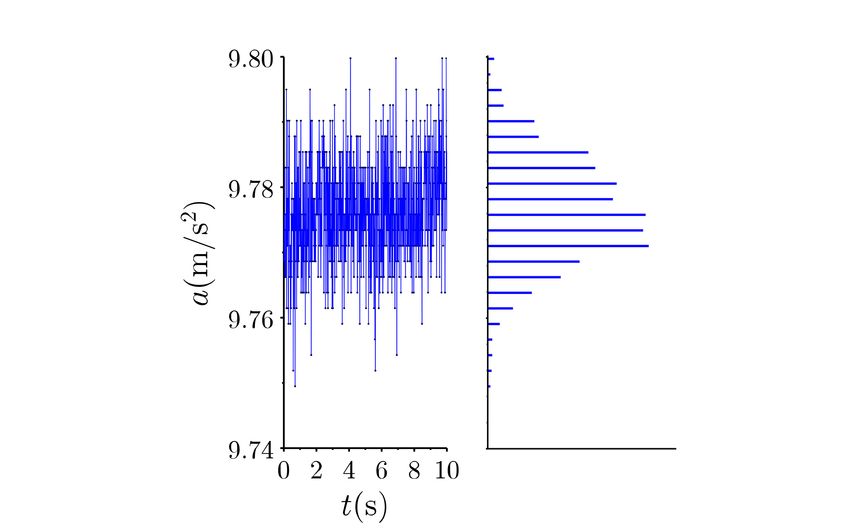
and, eventually, comparing them with those expected from a known distribution, typically a
normal distribution. Although these experiments are illustrative, most of them are tedious
and do not adequately reflect the present state of the art.

   In contrat with the expectable learning outcomes mentioned above, recent studies13–15
report several difficulties associated with error analysis among students. The study by Séré
et al 13 highlighted the lack of understanding of the need to make several measurements, the
poor insight into the notion of confidence intervals or the inability to distinguish between
random and systematic errors. Another investigation14 remarked the inconsistency of the
common view of students with generally accepted scientific models. On many occasions, the
student’s model of thinking is close to a point paradigm as opposed to a more elaborated
probabilistic interpretation of the measurements. A reseach-based assesment showed that
although the impact of introductory laboratory courses was positive, only a relatively small
percentage of students developed a deeper understanding of measurement uncertainty16 .

   The fluctuations present in the sensors of modern mobile devices give rise to an alternative
approach to teaching error analysis. Indeed, most smartphones and tablets come equipped
with several built-in sensors such as accelerometers, magnetometers, proximeters or ambient-
light sensors. Several Physics experiments using these sensors have been proposed in recent
years (see for example17–19 ). In almost all the experiments, only mean values are taken
into consideration; however, due to their sensitivity, sensor readings also display statistical
fluctuations. Although being detrimental in many situations, these fluctuations can be used
favorably to illustrate basic concepts related to the statistical treatment of measurements.
Using these sensors, it is certainly possible to acquire hundreds or thousands of repeated
values of a physical magnitude in a few seconds and analyze them in the mobile device or in
a PC. We propose here a set of laboratory activities to teach error analysis and uncertainties
in introductory Physics laboratories based on the fluctuations registered by mobile-device
sensors. In the next Section we describe the basic set of activities while Section III is focused
on other applications that take into account sensor fluctuations in non-standard situations.
Finally, in Section IV we present the summary and conclusion.

                                              3
II. A LABORATORY BASED ON MOBILE DEVICES
Among all the sensors, accelerometers, capable of measuring the acceleration of the de-
vice in the three independent spatial directions, are the most ubiquitous in mobile devices.
Though it is possible to use accelerometers or anyone of the others or even more than one
sensor simultaneously here, for the sake of clarity, the proposed experiments are mainly
based on the z component of the acceleration az , defined as perpendicular to the screen.
As a general rule, the characteristics of the sensors can be found using specific applications
(apps) or looking for datasheets in the internet. The range (difference between the maximum
and minimum value that it is capable of measuring) and the resolution (minimum difference
that the sensor can register, which is sometimes incorrectly termed as accuracy) of several
sensors are summarized in Table I. It is worth remarking that, although being universally
known as accelerometers, in fact, they are force sensors20,21 . Indeed, a device standing on a
table would register a value close to the gravitational acceleration in the vertical axis while
a free-falling device would register a value close to zero in the same axis.
Phone Sensor Range (m/s2 ) Resolution (m/s2 )
Samsung Galaxy S7 K6DS3TR ±78.4532 0.0023942017
LG G3 LGE ±39.226593 0.0011901855
Nexus 5 MPU-6515 ±19.613297 0.0005950928
iPhone 6 MPU-6700 - -
Samsung J6+ LSM6DSL ±39.2266 0.0011971008
Xiaomi Redmi Note7 ICM20607 ±78.4532 0.0011901855
Samsung Galaxy S9 LSM6DSL ±78.4532 0.0023942017
Samsung A20S ICM40607 ±78.4532 0.0023956299
TABLE I. Range and resolution of several common mobile devices obtained with the Androsensor
app. Notice that sensors can usually operate within different ranges ±2g, ±4g, ±8g,..., which are
set by the mobile-device manufacturer. The resolution depends on the choice of range.
In the case of the iPhone the manufacturer does not provides this information.
In general, a specific piece of software, or an app, is necessary. Digital stores offer many
apps that are able to communicate with the sensors. In particular, Physics Toolbox Suite22 ,
4Androsensor and PhyPhox23 , whose screenshots are shown in Fig. 1, are suitable for the
experiments proposed here. Using these apps it is possible to select the relevant sensors, and
to setup the parameters such as the duration of the time series and the sampling frequency.
The registered data can be analyzed directly on the smartphone screen or transferred to the
cloud and studied on a PC using a standard graphics package. Others useful characteristics
of these apps are the delayed execution and the remote access via wi-fi or browser. These
capabilities allow the experimenter to avoid touching or pushing the mobile device once the
experiments has started.
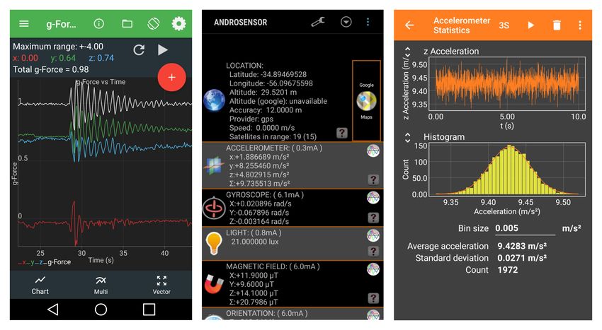
FIG. 1. Screenshots of three suitable apps: Physics Toolbox suite (left), Androsensor (center),
Phyphox (right). The right panel shows a Phyphox screenshot of the experiment Statistical Basics
including a temporal series of the vertical component of the acceleration (top) and the corre-
sponding histogram (bottom) overlapped with a Gaussian curve with the same mean and standard
deviation indicated in the image.
A. Normal distribution of the sensors’ fluctuations
The first experiment consists of recording the fluctuations of the vertical component of
the accelerometer sensor with the mobile device in three different situations: laid on a table,
hand-held and resting on another smartphone playing a 600 Hz pure tone. In all the cases, we
5choose, unless stated otherwise, a delay of 3 s and register az for 30 s. The delay is important
in order to avoid touching the device when the register starts and thus introducing spurious
values. Let us denote N the number of measurements registered by the sensor, az the mean
value and σaz the standard deviation.
The results of the experiment are summarized in Fig. 2 in which the top panels display the
temporal series, az (t), and the bottom panels show the histograms using the same respective
colors. In all the cases the accelerations fluctuate stationarily around mean values. Although
these values are close to the well-known value of the gravitational acceleration, they are
slightly different and they are not expected to represent a measure of that magnitude.
This is due to several reasons, for instance it depends on the horizontalitly of the table or
the hand or also on the calibration of the sensor. It is interesting for students to check
that the mean value changes when the device is laid on a table with the screen pointing
upwards or downwards. Another possible, and equivalent, alternative (not shown here)
consists of plotting ax (t) or ay (t) which exhibit similar temporal evolutions and histograms
but fluctuating around a value close to 0 m/s2 .
The differences in the intensity of the fluctuations exhibited in the three mentioned sit-
uations are evident in the top panels of Fig. 2. The intensity is clearly larger when the
smartphone is hand-held (red) or under the influence of the 600Hz tone (green) in compari-
son with the smartphone on a table (blue). The standard deviation of each series, indicated
in the legend boxes, is clearly related to the intensity of the fluctuations. This observa-
tion substantiates the use of the standard deviation in the framework of the applications
proposed in Section III.
A relevant aspect to study is the distribution of the fluctuations and how it compares
with the normal distribution. The firt approach to testing the normality of the distribution
is qualitative. In the bottom panels (Fig. 2), the histograms are compared with normal
(Gaussian) functions with the same mean values and standard deviation and the vertical
scale adjusted so that the area under the normal curve and the sum of the bins of the
histogram are equal. It can be observed that the histograms and normal functions agree
very well in the cases of the blue and red curves. By increasing the number of samples N
and simultaneously decreasing the width of the bins, it is possible to see that the agreement
improves even more (not shown here). Contrarily, in the green case, the pure tone breaks
the normality of the distributions as it is clearly revealed by the disagreement between the
6FIG. 2. Fluctuations registered by the accelerometer. The top panels display az (t) with the
device horizontal in three different situations: laid on a table (blue), hand-held (red) and resting
on another smartphone playing a 600 Hz pure tone (green). The smartphone was the LG-G3 with a
∆t = 0.004 s sampling period. The bottom panels display the histograms and the continuous lines
with the same color are normal (Gaussian) functions with same mean value, standard deviation
and normalization. Legend boxes indicate χ2 values, calculated with 8 bins, and the corresponding
confidence levels (CL).
histogram and normal curve.
The second and more quantitative approach to verifying the normality of the distributions
is given by the comparison of the fraction of observations in a given interval around the mean
value and the expected percentage according to a normal distribution. Table II displays these
percentages for the experiment depicted in Fig. 2. It can be seen that, in agreement with the
7qualitative test, the observed and expected percentages are quite similar when the device is
on the table or hand-held where they present considerable divergences under the influence
of the 600 Hz tone.
Experiment Table Hand Speaker Theoretical
N 3554 3579 3547 -
x ± σ (m/s2 ) 9.474 ± 0.019 9.362 ± 0.066 9.492 ± 0.054 -
(x − σ, x + σ) 69.3% 67.9% 58.2% 68.2%
(x − 2σ, x + 2σ) 95.2% 95.5% 99.2% 95.4%
(x − 3σ, x + 3σ) 99.7% 99.7% 100.0% 99.7%
TABLE II. Fraction of observations in intervals around the mean defined in units of the standard
deviation compared with the expected number according to a normal distribution. Each column
corresponds to each of the temporal series plotted in Fig. 2.
To gain further insight into the normality of the distributions, a chi-squared test compar-
ing the difference between the number of observations measured and expected in each bin1 ,
was performed. Each χ2 valued can be associated with a confidence level that determines
the rejection of the hypothesis of normal distribution. Clearly in the blue and red cases the
χ2 test indicates the compatibility of the normal distribution hypothesis while in the green
case this hypothesis must be rejected.
B. Resolution in digital sensors
By zooming in on the temporal series displayed in Fig. 2, it can be seen that the sensor
values do not take continuous values, but only a discrete set is possible. This is more
evident in the experiment displayed in Fig. 3 where the horizontal axis has been zoomed
out in the left panel, and a horizontal histogram with the same values is shown in the right
panel. The difference between the discrete values in the vertical axis is the resolution of
the instrument, that is, the minimum difference that the sensor can register. This is typical
of digital instruments, where a continuous magnitude (such as acceleration, in this case)
is transformed by a sensor into an analog electrical signal, which is in turn transformed
by an analog-to-digital converter (ADC) into a digital signal which can only take certain
8FIG. 3. Discrete nature of the sensor data. The horizontal axis in the left panel was zoomed
out to emphasize the discrete nature of the accelerometer values. The right panel shows the same
values in a horizontal histogram with the same vertical scale.
discrete values. In this case, the acceleration sensor of the Samsung S7 is a K6DS3TR and
its resolution, indicated in Table I, is δ = 0.0023942017 m/s2 which corresponds exactly to
the difference between consecutive acceleration values.
The resolution of the sensor, δ, is the quotient between the range, 2R, and the number
of different values that the sensor can register, 2n ,
2R
δ= (1)
2n
where n is the number of bits of the sensor and the factor 2 stands because it registers not
only positive measures, but also negative accelerations. Taking into consideration Table I,
it can be determined that this sensor is capable of measuring 2R/δ = 65536 different values
and since 65536 = 216 , this means that it is a 16-bit sensor, which can be easily verified on
the data sheets.
C. Standard error and optimal number of measurements
The standard deviation, if N is large enough, is characteristic of the set of all the possible
observations whereas the standard error, or standard deviation of the mean, generally defined
9N 563 1156 1746 2348 2941 3535 4166 4733 5327 5919
σaz (m/s2 ) 0.020 0.019 0.018 0.019 0.020 0.019 0.019 0.019 0.019 0.020
TABLE III. Standard deviations of az (t) corresponding to several experiments under identical
conditions but with different number of measurements.
√
as σ(a¯z ) = σaz / N represents the margin of uncertainty of the mean value obtained in a
particular set of measurements1 . The result of a specific measurement is usually expressed
as az ± σ(a¯z ) representing the best estimate and the confidence in that value. In Table. III
the standard deviation is shown as a function of N . As mentioned above, it is clear from
that data that σaz is nearly constant and, as a consequence, σ(a¯z ) is proportional to N −1/2 .
The choice of N in a specific experiment is a delicate question. Indeed, if we could repeat
the measurements infinite times the standard error would vanish and we could achieve a
perfect knowledge of the best estimate. However, as the decrease of the standard error with
the number of observations is slow, it is impractical to increment this number excesively.
A common criterion is to take a number of measurements, often referred as the optimal
number of measurements, Nopt , such that the statistical uncertainty is of the same order as
the systematic (or type B) errors. Here, in the absence of other sources of systematic errors,
the standard error should be of the same order as the resolution of the digital instrument:
p
σ(a¯z ) = σaz / Nopt ∼ δ. In the experiment depicted in Table III with a LG G3, the
resolution is δ = 0.0012 m/s2 , therefore Nopt ∼ 250.
III. OTHER APPLICATIONS
In this Section we propose a couple of activities in which the knowledge of the fluctuations
measured by a sensor can contribute to quantify another magnitude.
A. The steady hand game
An interesting experiment is to study the intensities of the fluctuations depending on
the way in which the experimenter holds his/her device. This activity can be adapted for
a group of students as a challenge consisting of trying to hold the device as steadily as
10FIG. 4. Comparative table of the standard deviation σ for different mobile devices in different
activities as a function of the different models (see Table I). Lines are guides for the eyes
possible. Another possibility (not recommended by the authors) is to study the fluctuations
of the gait of a pedestrian as a function of the alcohol beverage intake similar to24 .
The steadiness of the device is quantified by the standard deviation of a given temporal
series. The intensities of the fluctuations in different situations and for different sensors
are displayed in Fig. 4. It is evident from these values that the mobile device on the table
exhibits in all the cases less fluctuations than when the device is held by the experimenter.
Moreover a more stable position is achieved by keeping the device close to the trunk as
opposed to the classical selfie position. Another point worth mentioning is that the intensity
of the fluctuations depends on the specific sensor but exhibits in all cases the same trends
mentioned above. Several interesting extensions to this experiment can be proposed: the
dependence on the characteristics of the experimenter (age, training, concentration). The
origin of the fluctuations, mechanical or electronical, can be considered in case of having an
antivibration table. When using interferometric methods a precise calibration of the mobile
device sensor could also be performed.
11B. The smartphone as a way to assess road quality
Recently, smartphones’ sensors were proposed to assess road quality25 . In this activity,
which can be performed outdoors, students can assess the quality of a road. A means of
transport, in this case a car, is employed under similar conditions (speed), but other pos-
sibilities, such as a bike, are equally feasible. The intensities of the fluctuations traveling
by car on different roads are listed in Table IV. To get an insight of the fluctuations at-
tributable to the road the noise with the car stopped and the engine idle is indicated in the
first road. A similar measurement performed in a flying aircraft is included solely for the
sake of comparison. This activity can be extended to evaluate comfort in any other means
of transport media, for example, elevators.
Situation N σG3 (m/s2 ) N σXR7 (m/s2 )
Engine idle 1181 0.3818 4984 0.0352
Smooth pavement 1200 1.3487 4974 0.5642
Stone pavement - - 4952 1.1491
Aircraft 1999 0.4374 - -
TABLE IV. Assessment of the quality of different roads. Standard deviation of az while the device
is on the floor of the car with the screen orientated upwards.
IV. SUMMARY AND CONCLUSION
The activities discussed above were successfully proposed at our university to freshman
Engineering and Physics students. In previous laboratory experiments students already
knew the usefulness of the sensor to study several phenomena in which the noise was a factor
to avoid. However, when sensors were proposed to study fluctuations, they were surprised
to discover a kind of underlying world. Despite having gone through statistical topics in
several courses, the normal distribution appearing as an experimental fact rather than a
mathematical consequence, was original. It is worth discussing, how the distributions of the
other sensors change. For example, magnetometer fluctuations, significantly influenced by
motors or ferromagnetic material in the vicinity, do not follow normal distributions. Several
12challenges can be proposed in relation to sports, comfort evaluations or quality control.
The main conclusion is that modern mobile-device sensors are useful tools for teaching
error analysis and uncertainties. In this work we proposed several activities that can be
performed to teach uncertainties and error analysis using digital instruments and the builtin
sensors included in modern mobile devices. It is straightforward to obtain experimental
distributions of fluctuations and compare them with the expected ones. It is shown that the
distributions usually obey normal (Gaussian) statistics; however, it is easy to obtain non
normal distributions. The role of noise intensity, spreading or narrowing the distributions
open up the possibilities of new applications. Holding the mobile device in different ways
also gives an idea of how firmly it is held. Registering acceleration values in a car can
assess the smoothness of a road. In this approach, the lengthy and laborious manipulations
of traditional approaches based on repetitive measurements, are avoided allowing teaching
to focus on the fundamental concepts. These experiments could contribute to motivating
students and showing them the necessity of considering uncertainty analysis. Several possible
extensions related to non-normal statistics can be considered, such as Poison distribution8 ,
distribution of maxima, Chauvenet criterion26 , or Benford law27 .
ACKNOWLEDGMENT
The authors would like to thank PEDECIBA (MEC, UdelaR, Uruguay) and express their
gratitude for the grant Fisica Nolineal (ID 722) Programa Grupos I+D CSIC 2018 (UdelaR,
Uruguay).
∗ monteiro@ort.edu.uy
† marti@fisica.edu.uy
1 John Taylor. Introduction to error analysis, the study of uncertainties in physical measurements.
University Science Books, 1997.
2 Ifan Hughes and Thomas Hase. Measurements and their uncertainties: a practical guide to
modern error analysis. Oxford University Press, 2010.
3 OIML ISO. Guide to the expression of uncertainty in measurement (gum). Geneva, Switzerland,
1995.
134 Barry N Taylor, Peter J Mohr, and M Douma. The nist reference on constants, units, and
uncertainty. available online from:. physics. nist. gov/cuu/index, 2007.
5 Bureau International des Poids et Mesures. Evaluation of measurement data–guide to the
expression of uncertainty in measurement, 2008.
6 Joseph Kozminski, Heather Lewandowski, Nancy Beverly, Steve Lindaas, Duane Deardorff,
Ann Reagan, Richard Dietz, Randy Tagg, Jeremiah Williams, Robert Hobbs, et al. Aapt
recommendations for the undergraduate physics laboratory curriculum. American Association
of Physics Teachers, 29, 2014.
7 I. M. Meth and L. Rosenthal. An experimental approach to the teaching of the theory of
measurement errors. IEEE Transactions on Education, 9(3):142–148, 1966.
8 E. Mathieson and T. J. Harris. A student experiment on counting statistics. American Journal
of Physics, 38(10):1261–1262, 1970.
9 P. C. B. Fernando. Experiment in elementary statistics. American Journal of Physics, 44(5):460–
463, 1976.
10 Arvind, P. S. Chandi, R. C. Singh, D. Indumathi, and R. Shankar. Random sampling of an
alternating current source: A tool for teaching probabilistic observations. American Journal of
Physics, 72(1):76–82, 2004.
11 Tadeusz Wibig and Punsiri Dam-o. ‘hands-on statistics’—empirical introduction to measure-
ment uncertainty. Physics Education, 48(2):159–168, feb 2013.
12 K K Gan. A simple demonstration of the central limit theorem by dropping balls onto a grid
of pins. European Journal of Physics, 34(3):689–693, mar 2013.
13 Marie-Geneviève Séré, Roger Journeaux, and Claudine Larcher. Learning the statistical analysis
of measurement errors. International Journal of Science Education, 15(4):427–438, 1993.
14 Saalih Allie, Andy Buffler, Bob Campbell, Fred Lubben, Dimitris Evangelinos, Dimitris Psillos,
and Odysseas Valassiades. Teaching measurement in the introductory physics laboratory. The
Physics Teacher, 41(7):394–401, 2003.
15 MF Chimeno, MA Gonzalez, and J RAMOS Castro. Teaching measurement uncertainty to
undergraduate electronic instrumentation students. International Journal of Engineering Edu-
cation, 21(3):525–533, 2005.
16 Trevor S. Volkwyn, Saalih Allie, Andy Buffler, and Fred Lubben. Impact of a conventional
introductory laboratory course on the understanding of measurement. Phys. Rev. ST Phys.
14Educ. Res., 4:010108, May 2008.
17 Rebecca Vieyra, Chrystian Vieyra, Philippe Jeanjacquot, Arturo Marti, and Martı́n Monteiro.
Five challenges that use mobile devices to collect and analyze data in physics. The Science
Teacher, 82(9):32–40, 2015.
18 Katrin Hochberg, Jochen Kuhn, and Andreas Müller. Using smartphones as experimental
tools—effects on interest, curiosity, and learning in physics education. Journal of Science Edu-
cation and Technology, 27(5):385–403, 2018.
19 Martin Monteiro and Arturo C Marti. Using smartphone pressure sensors to measure vertical
velocities of elevators, stairways, and drones. Physics Education, 52(1):015010, 2017.
20 Martı́n Monteiro, Cecilia Cabeza, and Arturo C Martı́. Exploring phase space using smartphone
acceleration and rotation sensors simultaneously. European Journal of Physics, 35(4):045013,
2014.
21 Martı́n Monteiro, Cecilia Cabeza, and Arturo C. Marti. Acceleration measurements using
smartphone sensors: Dealing with the equivalence principle. Revista Brasileira de Ensino de
Fı́sica, 37:1303 –, 03 2015.
22 Rebecca Vieyra and Chrystian Vieyra. Physics toolbox suite, July 2019.
23 S Staacks, S Hütz, H Heinke, and C Stampfer. Advanced tools for smartphone-based experi-
ments: phyphox. Physics Education, 53(4):045009, may 2018.
24 Tirra Hanin Mohd Zaki, Musab Sahrim, Juliza Jamaludin, Sharma Rao Balakrishnan,
Lily Hanefarezan Asbulah, and Filzah Syairah Hussin. The study of drunken abnormal hu-
man gait recognition using accelerometer and gyroscope sensors in mobile application. In 2020
16th IEEE International Colloquium on Signal Processing & Its Applications (CSPA), pages
151–156. IEEE, 2020.
25 PM Harikrishnan and Varun P Gopi. Vehicle vibration signal processing for road surface mon-
itoring. IEEE Sensors Journal, 17(16):5192–5197, 2017.
26 Braden J Limb, Dalon G Work, Joshua Hodson, and Barton L Smith. The inefficacy of chau-
venet’s criterion for elimination of data points. Journal of Fluids Engineering, 139(5), 2017.
27 Jonathan R Bradley and David L Farnsworth. What is benford’s law? Teaching Statistics,
31(1):2–6, 2009.
15You can also read