What drives bitcoin? An approach from continuous local transfer entropy and deep learning classification models
←
→
Page content transcription
If your browser does not render page correctly, please read the page content below
What drives bitcoin? An approach from continuous local transfer
                                                     entropy and deep learning classification models
                                                                      Andrés García-Medina1,2,* and Toan Luu Duc Huynh3,4,5
                                                 1
                                                  Centro de Investigación en Matemáticas, Unidad Monterrey, Apodaca, 66628, Mexico
                                             2
                                                 Consejo Nacional de Ciencia y Tecnología, Cátedras Conacyt, Ciudad de México, 03940,
                                                                                        Mexico
                                                               3
                                                                 WHU - Otto Beisheim School of Management, Germany
                                                                 4
                                                                   University of Economics Ho Chi Minh City, Vietnam
                                                                             5
                                                                               IPAG Business School, France
                                                                    *
                                                                      Corresponding author: andres.garcia@cimat.mx
arXiv:2109.01214v1 [q-fin.ST] 2 Sep 2021

                                                                                               September 6, 2021

                                                                                                      Abstract
                                                         Bitcoin has attracted attention from different market participants due to unpredictable price patterns.
                                                     Sometimes, the price has exhibited big jumps. Bitcoin prices have also had extreme, unexpected crashes. We
                                                     test the predictive power of a wide range of determinants on bitcoins’ price direction under the continuous
                                                     transfer entropy approach as a feature selection criterion. Accordingly, the statistically significant assets
                                                     in the sense of permutation test on the nearest neighbour estimation of local transfer entropy are used as
                                                     features or explanatory variables in a deep learning classification model to predict the price direction of
                                                     bitcoin. The proposed variable selection methodology excludes the NASDAQ index and Tesla as drivers.
                                                     Under different scenarios and metrics, the best results are obtained using the significant drivers during the
                                                     pandemic as validation. In the test, the accuracy increased in the post-pandemic scenario of July 2020 to
                                                     January 2021 without drivers. In other words, our results indicate that in times of high volatility, Bitcoin
                                                     seems to autoregulate and does not need additional drivers to improve the accuracy of the price direction.

                                              Keywords: Econophysics, Behavioral Finance, Bitcoin, Transfer Entropy, Deep Learning

                                           Introduction
                                           Currently, there is tremendous interest in determining the dynamics and direction of the price of Bitcoin due
                                           to its unique characteristics, such as its decentralization, transparency, anonymity, and speed in carrying out
                                           international transactions. Recently, these characteristics have attracted the attention of both institutional
                                           and retail investors. Thanks to technological developments, investor trading strategies are benefited by digital
                                           platforms; therefore, market participants are more likely to digest and create information for this market. Of
                                           special interest is its decentralized character, since its value is not determined by a central bank but, essentially,
                                           only by supply and demand, recovering the ideal of a free market economy. At the same time, it is accessible to
                                           all sectors of society, which breaks down geographic and particular barriers for investors. The fact that there are
                                           a finite number of coins and the cost of mining new coins grows exponentially has suggested to some specialists
                                           that it may be a good instrument for preserving value. That is, unlike fiat money, Bitcoin cannot be arbitrarily
                                           issued, so its value is not affected by the excessive issuance of currency that central banks currently follow, or by
                                           low interest rates as a strategy to control inflation. In other words, it has been recently suggested that bitcoin
                                           is a safe-haven asset or store of value, having a role similar to that once played by gold and other metals.
                                               The study of cryptocurrencies and bitcoin has been approached from different perspectives and research
                                           areas. It has been addressed from the point of view of financial economics, econometrics, data science, and more
                                           recently by econophysics. In these approaches, various methodologies and mathematical techniques have been
                                           utilised to understand different aspects of these new financial instruments. These topics range from systemic
                                           risk, the spillover effect, autoscaling properties, collective patterns, price formation, and forecasting in general.
                                           Remarkable work in the line of multiscale analysis of cryptocurrency markets can be found in [39]. However, this
                                           paper is motivated by using the econphysics approach, incorporated with rigorous control variables to predict
                                           Bitcoin price patterns. We would like to offer a comprehensive review of the determinants of Bitcoin prices. The
                                           first pillar can be defined as sentiment and social media content. While Bitcoin is widely considered a digital
financial asset, investors pay attention to this largest market capitalization by searching its name. Therefore,
the strand of literature on Google search volume has become popular for capturing investor attention [38].
Concomitantly, not only peer-to-peer sentiment (individual Twitter accounts or fear from investors) [36, 6] but
also influential accounts (the U.S. President, media companies) [18, 10, 7] significantly contribute to Bitcoin price
movement. Given the greatest debate on whether Bitcoin should act as a hedging, diversifying or safe-haven
instrument, Bitcoin exhibits a mixture of investing features. More interestingly, uncertain shocks might cause
changes in both supply and demand in Bitcoin circulation, implying a change in its prices [14]. Thus, the diverse
stylized facts of Bitcoin, including heteroskedasticity and long memory, require uncertainty to be controlled in
the model. While uncertainties represent the amount of risk (compensated by the Bitcoin returns)[2], our
model also includes the price of risk, named the ‘risk aversion index’ [3]. These two concepts (amount of risk
and the price of risk) demonstrate discount rate factors in the time variation of any financial market [11]. In
summary, the appearance of these determinants could capture the dynamics of the cryptocurrency market.
Since cryptocurrency is a newly emerging market, the level of dependence in the market structure is likely
higher than that in other markets [28]. Furthermore, the contagion risk and the connectedness among these
cryptocurrencies could be considered the risk premium for expected returns [31, 20]. More importantly, this
market can be driven by small market capitalization, implying vulnerability of the market [21]. Hence, our
model should contain alternative coins (altcoins) to capture their movements in the context of Bitcoin price
changes. Finally, investors might consider the list of these following assets as alternative investment, precious
metals being the first named. They are not only substitute assets [37] but also predictive factors (for instance,
gold and platinum) [19], which additionally include commodity markets (such as crude oil [22, 23], exchange
rate [9], equity market [29]), and Tesla’s owner [1]). In summary, there are voluminous determinants of Bitcoin
prices. In the scope of this study, we focus on the predictability of our model, especially the inclusion of social
media content, representing the high popularity of information, on the Bitcoin market. However, the more
control variables there are, the higher the accuracy of prediction. Our model thus may be a useful tool by
combining the huge predictive factors for training and forecasting the response dynamics of Bitcoin to other
relevant information.
This study approaches Bitcoin from the framework of behavioural and financial economics using an approach
from econophysics and data science. In this sense, it seeks to understand the speculative character and the
possibilities of arbitrage through a model that includes investor attention and the effect of the news, among
other factors. For this, we will use a causality method originally proposed by Schreiber [35], and we will use
the information as characteristics of a deep learning model. The current literature only focuses on specific
sentiment indicators (such as Twitter users [36] or the number of tweets [33, 32]), and our study crawled the
original text from influential Twitter social media users (such as the President of United States, CEO of Tesla,
and well-known organizations such as the United Nations and BBC Breaking News). Then, we processed
language analyses to construct the predictive factor for Bitcoin prices. Therefore, our model incorporates a new
perspective on Bitcoin’s drivers.
In this direction, the work of [25] uses the effective transfer entropy as an additional feature to predict
the direction of U.S. stock prices under different machine learning approaches. However, the approximation
is discrete and based on averages. Furthermore, the employed metrics are not exhaustive to determine the
predictive power of the models. In a similar vein, the authors of [15] perform a comparative analysis of machine
learning methods for the problem of measuring asset risk premiums. Nevertheless, they do not take into account
recurrent neural network models or additional nontraditional features. Furthermore, an alternative approach to
study the main drivers of Bitcoin is discussed in [27], where the author explores wavelet coherence to examine
the time and frequency domains between short- and long-term interactions.
Our study embodied a wide range of Bitcoin’s drivers from alternative investment, economic policy un-
certainty, investor attention, and so on. However, social media is our main contribution to predictive factors.
Specifically, we study the effect that a set of Twitter accounts belonging to politicians and millionaires has on the
behaviour of Bitcoin’s price direction. In this work, the statistically significant drivers of Bitcoin are detected
in the sense of the continuous estimation of local transfer entropy (local TE) through nearest neighbours and
permutation tests. The proposed methodology deals with non-Gaussian data and nonlinear dependencies in the
problem of variable selection and forecasting. One main aim is to quantify the effects of investor attention and
social media on Bitcoin in the context of behavioural finance. Another aim is to apply classification metrics to
indicate the effects of including or not the statistically significant features in an LSTM’s classification problem.
Results
This section describes the data under study, the variable selection procedure, and the main findings on Bitcoin
price direction.
2Data
An important part of the work is the acquisition and preprocessing of data. We focus on the period of time
from 01 January 2017 to 09 January 2021 at a daily frequency for a total of n = 1470 observations. As a
priority, we consider the variables listed in Supplementary Table S1 as potential drivers of the price direction
of Bitcoin (BTC). Investor attention is considered Google Trends with the query="Bitcoin". Additionally,
the number of mentions is properly scaled to make comparisons between days of different months because by
default, Google Trends weighs the values by a monthly factor. Then, the log return of the resulting time series
is calculated. The social media data are collected from the Twitter API (https://developer.twitter.com/
en/docs/twitter-api). Nevertheless, the API of Twitter only enables downloading the latest 3,200 tweets
of a public profile, which generally was not enough to cover the period of study. Then, the dataset has been
completed with the freely available repository of https://polititweet.org/. In this way, the collected number
of tweets was 21,336, 22,808, 24,702, 11,140, and 26,169 for each of the profiles listed in Supplementary Table S1
in the social media type, respectively. The textual data of each tweet in the collected dataset are transformed
to a sentiment polarity score through the VADER lexicon [17]. Then, the scores are aggregated daily for each
profile. The resulting daily time series have missing values due to the inactivity of the users, and then a
third-order spline is considered before calculating their differences. The last is to stationarize the polarity time
series. It is important to remember that Donald Trump’s account was blocked on 8 January 2021, so it was also
necessary to impute the last value to have series of the same length.
The economic policy uncertainty index is a Twitter-based uncertainty index (Twitter-EPU). The creators
of the index used the Twitter API to extract tweets containing keywords related to uncertainty ("uncertain",
"uncertainly", "uncertainties", "uncertainty") and economy ("economic", "economical", "economically", "eco-
nomics", "economies", "economist", "economists", "economy"). Then, we use the index consisting of the
total number of daily tweets containing inflections of the words uncertainty and economy (Please consult
https://www.policyuncertainty.com/twitter_uncert.html for further details of the index). The risk aver-
sion category considers the financial proxy to risk aversion and economic uncertainty proposed as a utility-based
aversion coefficient [3]. A remarkable feature of the index is that in early 2020, it reacted more strongly to the
new COVID-19 infectious cases than did a standard uncertainty proxy.
As complementary drivers, it includes a set of highly capitalized cryptocurrencies and a heterogeneous port-
folio of financial indices. Specifically, Ethereum (ETH), Litecoin (LTC), Ripple (XRP), Dogecoin (DOGE),
and the stable coin TETHER are included from yahoo finance (https://finance.yahoo.com/). The com-
ponents of the heterogeneous portfolio are listed in Supplementary Table S1, which takes into account the
Chicago Board Options Exchange’s CBOE Volatility Index (VIX). This last information was extracted from
Bloomberg (https://www.bloomberg.com/). It is important to point out that risk aversion and the financial
indices do not have information that corresponds to weekends. The imputation method to obtain a complete
database consisted of repeated Friday values as a proxy for Saturday and Sunday. Then, the log return of the re-
sulting time series is calculated. This last transformation was also made for Twitter-EPU and cryptocurrencies.
The complete dataset can be found in the Supplementary Information.
Usually, the econophysics and data science approaches share the perspective of observing data first and
then modelling the phenomena of interest. In this spirit, and with the intention of gaining intuition on the
problem, the standardized time series (target and potential drivers), as well as the cumulative return of the
selected cryptocurrencies and financial assets (see Supplementary Figs. S1 and S2, respectively) are plotted.
The former figure shows high volatility in almost all the studied time series around March 2020, which might
be due to the declaration of the pandemic by the World Health Organization (WHO) and the consequent fall
of the worlds main stock markets. The latter figure exhibits the overall best cumulative gains for BTC, ETH,
LTC, XRP, DOGE, and Tesla. It is worth noting that the only asset with a comparable profit to that of the
cryptocurrencies is Tesla, which reaches high cumulative returns starting at the end of 2019 and increases its
uptrend immediately after the announcement of the worldwide health emergency. Furthermore, Fig. 1 shows the
heatmap of the correlation matrix of the preprocessed dataset. We can observe the formation of certain clusters,
such as cryptocurrencies, metals, energy, and financial indices, which tells us about the heterogeneity of the data.
It should also be noted that the VIX volatility index is anti-correlated with most of the variables. Additionally,
the main statistical descriptors of the data are presented in Table 1. The first column is the variable’s names
or tickers. The subsequent columns represent the mean, standard deviation, skewness, kurtosis, Jarque Bera
test (JB), and the associated p value of the test for each variable, i.e., target, and potential drivers. Basically,
none of the time series passes the test of normality distribution, and most of them present a high kurtosis,
which is indicative of heavy tail behaviour. Finally, stationarity was checked in the sense of Dickey-Fuller and
the Phillips-Perron unit root tests, where all variables pass both tests.
3Variable selection
Given the observed characteristics of the data in the previous section, it is more appropriate to use a non-
parametric approach to determine the significant features to be employed in the predictive classification model.
Therefore, the variable selection procedure consisted of applying the continuous transfer entropy from each
driver to Bitcoin using the nearest neighbour estimation known as KSG estimation citeKraskov2004. Figure 2
shows the average transfer entropy when varying the Markov order k, l and neighbour parameter K from one
to ten for a total of 1,000 different estimations by each driver. The higher the intensity of the colour, the higher
the average transfer entropy (measured in nats). The grey cases do not transfer information to BTC. In other
words, these cases do not show a statistically significant flow of information, where the permutation test is
applied to construct 100 surrogate measurements under the null hypothesis of no directed relationship between
the given variables.
The tuple of parameters {k, l, K} that give the highest average transfer entropy from each potential driver
to BTC are considered optimal, and the associated local TE is kept as a feature in the classification model of
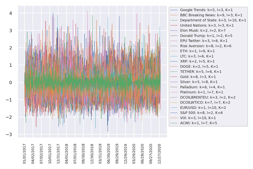
Bitcoin’s price direction. Figure 3 shows the local TE from each statistically significant driver to BTC at the
optimal parameter tuple {k, l, K}. Note that the set of local TE time series is limited to 23 features. Conse-
quently, the set of originally proposed potential drivers is reduced from 25 to 23. Surprisingly, NASDAQ and
Tesla do not send information to BTC for any value of {k, l, K} in the grid of the 1,000 different configurations.
Bitcoin’s price direction
The task of detecting Bitcoin’s price direction was done through a deep learning approach. The first step
consisted of splitting the data into training, validation, and test datasets. The chosen training period runs
from 1 January 2017 to 4 January 2020, or 75% of the original entire period of time, and is characterized as
a prepandemic scenario. The validation dataset is restricted to the period from 5 January 2020 to 11 July
2020, or 13% of the original data, and is considered the pandemic scenario. The test dataset involves the
postpandemic scenario from 12 July 2020 to 9 January 2021 and contains 12% of the complete dataset. Deep
learning forecasting requires transforming the original data into a supervised data set. Here, samples of 74
historical days and a one-step prediction horizon are given to the model to obtain a supervised training dataset,
with the first dimension being a power of two, which is important for the hyperparameter selection of the batch
dimension. Specifically, the sample dimensions are 1024, 114, and 107 for training, validation, and testing,
respectively. Because we are interested in predicting the direction of BTC, the time series are not demeaned
and instead are only scaled by their variance when feeding the deep learning models. An important piece in a
deep learning model is the selection of the activation function. In this work, the rectified linear unit (ReLU)
was selected for the hidden layers, which is defined as max(x, 0), where x is the input value. Then, for the
output layer, the sigmoid function is chosen because we are dealing with a classification problem. Explicitly,
this function takes the form σ(x) = 1/(1 + exp(−x)). Therefore, the appropriate loss function to monitor is the
PN
binary cross-entropy defined as Hp (q) = − N1 i=1 xi log(p(xi ))+(1−xi ) log(1−p(xi )). In addition, an essential
ingredient is the selection of the stochastic gradient descent method. Here, Adam optimization is selected based
on adaptive estimation of the first- and second-order moments. In particular, we used version [34] to search for
the long-term memory of past gradients to improve the convergence of the optimizer.
There exist several hyperparameters to take into account when modelling a classification problem under a
deep learning approach. These hyperparameters must be calibrated on the training and validation datasets to
obtain reliable results on the test dataset. The usual procedure to set them is via a grid search. Nevertheless,
deeper networks with more computational power are necessary to obtain the optimal values in a reasonable
amount of time. To avoid excessive time demands, we vary the most crucial parameters in a small grid and apply
some heuristics when required. The number of epochs, i.e., the number of times that the learning algorithm
will pass through the entire training dataset, is selected under the early stopping procedure. It consists of
monitoring a specific metric, in our case the binary accuracy. Thus, if for a predefined number of steps, the
metric does not decrease, we consider the number of epochs at which the binary accuracy reaches its highest
values as optimal. Another crucial hyperparameter is the batch, or the number of samples to work through
before updating the internal weight of the model. For this parameter the selected grid was {32, 64, 128, 256}.
Additionally, we consider the initial learning rates at which the optimizer starts the algorithm, which were
{0.001, 0.0001}. As an additional method of regularization, the effect of dropping between consecutive layers
is added. This value can take values from 0 to 1. Our grid for this hyperparameter is {0.3, 0.5, 0.7}. Finally,
because of the stochastic nature of the deep learning models, it is necessary to run several realizations and
work with averages. We repeat the hyperparameter selection with ten different random seeds for robustness.
The covered scenarios are the following: univariate (S1), where bitcoin is self-driven; all features (S2), where
all the potential drivers listed in table 1 are included as features of the model; significative features (S3), only
statistically significant drivers under the KSG transfer entropy approach are considered as features; local TE,
only the local TE of the statistically significant drivers are included as a feature; and finally the significative
4features + local TE (S5) scenario, which combines scenarios (S3) and (S4). Finally, five different designs
have been proposed for the architectures of the neural networks, which are denoted as deep LSTM (D1), wide
LSTM (D2), deep bidirectional LSTM (D3), wide bidirectional LSTM (D4), and CNN (D5). The specific designs
and diagrams of these architectures are displayed in Supplementary Fig. S3. In total, 6,000 configurations or
models were executed, which included the grid search for the optimal hyperparameters, the different scenarios
and architectures, and the realizations on different seeds to avoid biases due to the stochastic nature of the
considered machine learning models.
Tables 2 and 3 present the main results for the validation and test datasets, respectively. The results are
in terms of the different metrics explained in the Methods section and are the average of ten realizations as
previously explained. Table 2 explicitly states the best value for the dropout, learning rate (LR), and batch
hyperparameters. In both tables, the hashtag (#) column indicates the number of times the specific scenario
gives the best score for the different metrics considered so far. Hence, the architecture design D3 for case S3
yields the highest number of metrics with the best scores in the validation dataset. In contrast, in the test
dataset, the highest number of metrics with the best scores correspond to design D2 for case S1. Nevertheless,
design D5 from case S5 is close in the sense of the # value, where it presents the best AUC and PPV scores.
Discussion
We start from descriptive statistics as a first approach to intuitively grasp the complex nature of Bitcoin, as
well as its proposed heterogeneous drivers. As expected, the variables did not satisfy the normality assumption
and presented high kurtosis, highlighting the need to use nonparametric and nonlinear analyses.
The KSG estimation of TE found a consistent flow of information from the potential drivers to Bitcoin
through the considered range of K nearest neighbours. Even when, in principle, the variance of the estimate
decreases with K, the results obtained with K = 1 do not change abruptly for larger values. In fact, the
variation in the structure of the TE matrix for different Markov orders k, l is more notorious. Additionally,
attention must be paid to the evidence about the order k = l = 1 through values near zero. Practitioners
usually assume this scenario under Gaussian estimations. A precaution must then be made about the memory
parameters of Markov, at least when working with the KSG estimation. The associated local TE does not show
any particular pattern beyond high volatility, reaching values of four nats when the average is below 0.1. Thus,
volatility might be a better proxy for price fluctuations in future studies.
In terms of intuitive explanations, we found that the drivers of Bitcoin might not truly capture its returns
in distressed periods. Although we expected to witness that the predictive power of these determinants might
play an important role across time horizons, it turns out that the prediction model of Bitcoin relies on a choice
of a specific period. Thus, our findings also confirm the momentum effect that exists in this market [13]. Due
to the momentum effect, the timing of market booms could not truly be supported much for further analysis
by our models. In regard to our main social media hypothesis, the popularity of Bitcoin content still exists
as the predictive component in the model. More noticeably, our study highlights that Bitcoin prices can be
driven by momentum on social media [33]. However, the selection of training and testing periods should be
cautious with the boom and burst of this cryptocurrency. Apparently, while the fundamental value of Bitcoin
is still debatable [8], using behavioural determinants could have some merits in predicting Bitcoin. Thus, we
believe that media content would support the predictability of Bitcoin prices alongside other financial indicators.
Concomitantly, after clustering these factors, we found that the results seem better able to provide insights into
Bitcoin’s drivers.
On the other hand, the forecasting of Bitcoin’s price direction improves in the validation set but not for
all metrics in the test dataset when including significant drivers or local TE as a feature. Nonetheless, the
last assertion relies on the number of metrics with the best scores. Although the test dataset having the best
performance corresponds to the deep bidirectional LSTM (D3) for the scenario univariate (S3), this case only
beat three of the eight metrics. The other five metrics are outperformed by scenarios including significative
features (S3) and significative features + local TE (S5). Furthermore, the second-best performances are tied
with two of the eight metrics with leading values. Interestingly, the last case shows the best predictive power on
the CNN model using significant features as well as local TE indicators (D5-S5). In particular, it outperforms
the AUC and PPV overall. Moreover, it is important to note that the selected test period is atypical in the sense
of a bull period for Bitcoin as a result of the turbulence generated by the COVID-19 public health emergency;
this might induce safe haven behaviour related to this asset and increase its price and capitalization. This
atypical behaviour opens the door to propose future work to model Bitcoin by the self-exciting process of the
Hawkes model during times of great turbulence.
We would like to end by emphasizing that we were not exhaustive in modelling classification forecasting. In
contrast, our intention was to exemplify the effect of including the significant features and local TE indicators
under different configurations of a deep learning model through a variety of classification metrics. Two method-
ological contributions to highlight are the use of nontraditional indicators such as market sentiment, as well as
5a continuous estimation of the local TE as a tool to determine additional drivers in the classification model.
Finally, the models presented here are easily adaptable to high-frequency data because they are nonparametric
and nonlinear in nature.
Methods
Transfer Entropy
Transfer Entropy (TE) [35] measures the flow of information from system Y over system X in a nonsymmetric
way. Denote the sequences of states of systems X, Y in the following way: xi = x(i) and yi = y(i), i = 1, . . . , N .
The idea is to model the signals or time series as Markov systems and incorporate the temporal dependencies
by considering the states xi and yi to predict the next state xi+1 . If there is no deviation from the generalized
Markov property p(xi+1 |xi , yi ) = p(xi+1 |xi ), then Y has no influence on X. Hence, TE is derived using the last
idea and defined as
(k) (l)
X (k) (l) p(xi+1 |xi , yi )
TY →X (k, l) = p(xi+1 , xi , yi ) log (k)
, (1)
p(xi+1 |xi )
(k) (l)
where xi = (xi , . . . , xi−k+1 ) and yi = (yi , . . . , yi−l+1 ).
TE can be thought of as a global average or expected value of a local transfer entropy at each observation.
The procedure is based on the following arguments. TE can be expressed as a sum over all possible state
(k) (l)
transition ui = (xi+1 , xi , yi ) tuples and considers the probability of observing each such tuple [30] as the
weight factor. The probability p(ui ) is equivalent to counting the observations c(ui ) of ui and dividing by the
total number of observations. Then, if the count is replaced by its definition in the TE equation and it is
observed that the double summation runs over each observation a for each possible tuple observation ui , then
the expression is equivalent to a single summation over the N observations
(k) (l) c(u ) (k) (l) c(u ) (k) (l) N (k) (l)
X p(xi+1 |xi , yi ) 1 X Xi p(xi+1 |xi , yi ) 1 X Xi p(xi+1 |xi , yi ) 1 X p(xi+1 |xi , yi )
p(ui ) log (k)
= 1 log (k)
= log (k)
= log (k)
ui p(xi+1 xi ) N u a=1 p(xi+1 xi ) N u a=1 p(xi+1 xi ) N i=1 p(xi+1 xi )
i i
(2)
Therefore, TE is expressed as the expectation value of a local transfer entropy at each observation
(k) (l)
p(xi+1 |xi , yi )
TY →X (k, l) = log (k)
(3)
p(xi+1 xi )
The main characteristic of the local version of TE is to be measured at each time n for each destination element
X in the system and each causal information source Y of the destination. It can be either positive or negative
(k) (l)
for a specific event set (xi+1 , xi , yi ), which gives the opportunity to have a measure of informativeness or
noninformativeness at each point of a pair of time series.
On the other hand, there exist several approximations to estimate the probability transition distributions
involved in TE expression. Nevertheless, there is not a perfect estimator. It is generally impossible to minimize
both the variance and the bias at the same time. Then, it is important to choose the one that best suits the
characteristics of the data under study. That is the reason finding good estimators is an open research area [4].
This study followed the Kraskov-Stögbauer-Grassberger) KSG estimator [26], which focused on small samples
for continuous distributions. Their approach is based on nearest neighbours. Although obtaining insight into
this estimator is not easy, we will try it in the following.
Let X = (x1 , x2 , . . . , xd ) now denote a d-dimensional continuous random variable whose probability density
function is defined as p : Rd → R. The continuous or differential Shannon entropy is defined as
Z
H(X) = − p(X) log p(X)dX (4)
Rd
The KSG estimator aims to use similar length scales for K-nearest-neighbour distance in different spaces, as in
the joint space to reduce the bias [12].
To obtain the explicit expression of the differential entropy under the KSG estimator, consider N i.i.d.
samples χ = {X(i)}N i=1 , drawn from p(X). Beneath the assumption that i,K is twice the (maximum norm)
distance to the k-th nearest neighbour of X(i), the differential entropy can be estimated as
N
d X
ĤKSG,K (X) ≡ ψ(N ) − ψ(K) + log i,K , (5)
N i=1
6where ψ is known as the digamma function and can be defined as the derivative of the logarithm of the gamma
function Γ(x)
1 dΓ(K)
ψ(K) = (6)
Γ(K) dK
The parameter K defines the size of the neighbourhood to use in the local density estimation. It is a free
parameter, but there exists a trade-off between using a smaller or larger value of K. The former approach should
be more accurate, but the latter reduces the variance of the estimate. For further intuition, Supplementary
Fig. S4 graphically shows the mechanism for choosing the nearest neighbours at K = 3. Now, the KSG estimator
of TE can be derived based on the previous estimation of the differential entropy. First, TE has an alternative
representation as a sum of mutual information terms
k
TY →X (k, l) = I(Xi−1 l
: Yi−1 k
: Xi ) − I(Xi−1 l
: Yi−1 k
) − I(Xi−1 : Xi ). (7)
Second, consider the general expression for the mutual information of X and Y conditioned on Z, which is
written as a sum of differential entropy elements
I(X : Y |Z) = H(X, Z) + H(Y, Z) − H(X, Y, Z) − H(Z) (8)
Third, analogous to the KSG differential estimation, now taking into account a single ball for the Kth nearest
neighbours in the joint space, {x, y, z}, leads to
I(X : Y, Z) = ψ(K) − E{ψ(nxz ) − ψ(nyz ) − ψ(nz )}, (9)
where ε is the maximum norm to the Kth nearest neighbour in the joint space {x, y, z}; nz is the neighbour
count within norm ε in the z marginal space; and nxz and nyz are the neighbour counts within maximum norms
of ε in the joint {x, z} and {y, z} spaces, respectively. Finally, by substituting Eq. 9 into Eq. 7, we arrive at an
expression for the KSG estimator of TE.
In most cases, as analysed in this work, no analytic distribution is known. Hence, the distribution of
TYs →X (k, l) must be computed empirically, where Ys denotes the surrogate time series of Y . This is done by a
resampling method, creating a large number of surrogate time-series pairs {Ys , X} by shuffling (for permutations
or redrawing for bootstrapping) the samples of Y. In particular, the distribution of TYs →X (k, l) is computed by
permutation, under which surrogates must preserve p(xn+1 |xn ) but not p(xn+1 |xn , yn ).
Deep Learning Models
We can think of artificial neural networks (ANNs) as a mathematical model whose operation is inspired by
the activity and interactions between neuronal cells due to their electrochemical signals. The main advantages
of ANNs are their nonparametric and nonlinear characteristics. The essential ingredients of an ANN are the
neurons that receive an input vector xi , and through the point product with a vector of weights w, generate an
output via the activation function g(·):
f (xi ) = g(xu · w) + b, (10)
where b is a trend to be estimated during the training process. The basic procedure is the following. The first
layer of neurons or input layer receives each of the elements of the input vector xi and transmits them to the
second (hidden) layer. The next hidden layers calculate their output values or signals and transmit them as an
input vector to the next layer until reaching the last layer or output layer, which generates an estimation for an
output vector.
Further developments of ANNs have brought recurrent neural networks (RNNs), which have connections
in the neurons or units of the hidden layers to themselves and are more appropriate to capture temporal
dependencies and therefore are better models for time series forecasting problems. Instead of neurons, the
composition of an RNN includes a unit, an input vector xt , and an output signal or value ht . The unit is designed
with a recurring connection. This property induces a feedback loop, which sends a recurrent signal to the unit
as the observations in the training data set are analysed. In the internal process, backpropagation is performed
to obtain the optimal weights. Unfortunately, backpropagation is sensitive to long-range dependencies. The
involved gradients face the problem of vanishing or exploding. Long-short-term memory (LSTM) models were
introduced by Hochreiter and Schmidhuber [16] to avoid these problems. The fundamental difference is that
LSTM units are provided with memory cells and gates to store and forget unnecessary information.
Specifically, LSTM is composed of a memory cell (ct ), an input gate (it ), a forget gate (gt ), and an output
gate (ot ). Supplementary Fig. S5 describes the elements of a single LSTM unit. At time t, xt represents
the input, ht the hidden state, and c̃t the modulate gate, which is a value that determines how much new
7information is received or discarded in the cell state. The internal process of the LSTM unit can be described
mathematically by the following formula:
gt = σ(Ug xt + Wg ht−1 + bf ) (11)
it = σ(Ui xt + Wi ht−1 + bi ) (12)
c̃t = tanh(Ux xt + Wc ht−1 + bc ) (13)
ct = gt ∗ ct−1 + it ∗ c̃t (14)
ot = σ(Uo xt + Wo ht−1 bo ) (15)
ht = ot ∗ tanh(ct ) (16)
where U and W are weight matrixes, b is a bias term, and the symbol * denotes elementwise multiplication [24].
The final ANNs we need to discuss are convolutional neural networks (CNNs). They can be thought of as a
kind of ANN that uses a high number of identical copies of the same neuron. This allows the network to express
computationally large models while keeping the number of parameters small. Usually, in the construction of
these types of ANNs, a max-pooling layer is included to capture the largest value over small blocks or patches
in each feature map of previous layers. It is common that CNN and pooling layers are followed by a dense fully
connected layer that interprets the extracted features. Then, the standard approach is to use a flattened layer
between the CNN layers and the dense layer to reduce the feature maps to a single one-dimensional vector [5].
Classification Metrics
In classification problems, we have the predicted class and the actual class. The possible scenarios under a
classification prediction are given by the confusion matrix. They are true positive (TP), true negative (TN),
false positive (FP), and false negative (FN). Based on these quantities, it is possible to define the following
classification metrics:
• Accuracy = T P +T N
T P +T N +F P +F N
• Sensitivity, recall or true positive rate (TPR) = TP
T P +F N
• Specificity, selectivity or true negative rate (TNR) = TN
T N +F P
• Precision or Positive Predictive Value (PPV) = TP
T P +F P
• False Omission Rate (FOR) = FN
F N +T N
• Balanced Accuracy (BA) = T P R+T N R
2
P P V +T P R .
• F1 score = 2 P P V ×T P R
The most complex measure is the area under the curve (AUC) of the receiver operating characteristic (ROC),
where it expresses the pair (T P Rτ , 1 − T N Rτ ) for different thresholds τ . Contrary to the other metrics, the
AUC of the ROC is a quality measure that evaluates all the operational points of the model. A model with the
aforementioned metric higher than 0.5 is considered to have predictive power.
References
[1] Lennart Ante. “How Elon Musk’s Twitter Activity Moves Cryptocurrency Markets”. In: Available at SSRN
3778844 (2021).
[2] Scott R Baker, Nicholas Bloom, and Steven J Davis. “Measuring economic policy uncertainty”. In: The
quarterly journal of economics 131.4 (2016), pp. 1593–1636.
[3] Geert Bekaert, Eric C Engstrom, and Nancy R Xu. The Time Variation in Risk Appetite and Uncertainty.
Working Paper 25673. National Bureau of Economic Research; http://www.nber.org/papers/w25673,
2019.
[4] Terry Bossomaier et al. An introduction to transfer entropy. Springer, 2016, pp. 78–82.
[5] Jason Brownlee. Deep learning for time series forecasting: predict the future with MLPs, CNNs and LSTMs
in Python. Machine Learning Mastery, 2018.
[6] Tobias Burggraf et al. “Do FEARS drive Bitcoin?” In: Review of Behavioral Finance 13.3 (2020), pp. 229–
258.
8[7] Stefano Cavalli and Michele Amoretti. “CNN-based multivariate data analysis for bitcoin trend prediction”.
In: Applied Soft Computing 101 (2021), p. 107065.
[8] Pedro Chaim and Márcio P Laurini. “Is Bitcoin a bubble?” In: Physica A: Statistical Mechanics and its
Applications 517 (2019), pp. 222–232.
[9] Jeffrey Chu, Saralees Nadarajah, and Stephen Chan. “Statistical analysis of the exchange rate of bitcoin”.
In: PloS one 10.7 (2015), e0133678.
[10] Shaen Corbet et al. “The impact of macroeconomic news on Bitcoin returns”. In: The European Journal
of Finance 26.14 (2020), pp. 1396–1416.
[11] Sonali Das et al. “The effect of global crises on stock market correlations: Evidence from scalar regressions
via functional data analysis”. In: Structural Change and Economic Dynamics 50 (2019), pp. 132–147.
[12] Shuyang Gao, Greg Ver Steeg, and Aram Galstyan. “Efficient estimation of mutual information for strongly
dependent variables”. preprint at https://arxiv.org/abs/1411.2003. 2015.
[13] Klaus Grobys and Niranjan Sapkota. “Cryptocurrencies and momentum”. In: Economics Letters 180
(2019), pp. 6–10.
[14] Marc Gronwald. “Is Bitcoin a Commodity? On price jumps, demand shocks, and certainty of supply”. In:
Journal of International Money and Finance 97 (2019), pp. 86–92.
[15] Shihao Gu, Bryan Kelly, and Dacheng Xiu. “Empirical asset pricing via machine learning”. In: The Review
of Financial Studies 33.5 (2020), pp. 2223–2273.
[16] Sepp Hochreiter and Jürgen Schmidhuber. “Long Short-Term Memory”. In: Neural Computation 9.8 (Nov.
1997), pp. 1735–1780.
[17] Clayton Hutto and Eric Gilbert. “Vader: A parsimonious rule-based model for sentiment analysis of social
media text”. In: Proceedings of the International AAAI Conference on Web and Social Media 8.1 (2014),
pp. 216–225.
[18] Toan Luu Duc Huynh. “Does Bitcoin React to Trump’s Tweets?” In: Journal of Behavioral and Experi-
mental Finance 31 (2021), p. 100546.
[19] Toan Luu Duc Huynh, Tobias Burggraf, and Mei Wang. “Gold, platinum, and expected Bitcoin returns”.
In: Journal of Multinational Financial Management 56 (2020), p. 100628.
[20] Toan Luu Duc Huynh, Sang Phu Nguyen, and Duy Duong. “Contagion risk measured by return among
cryptocurrencies”. In: International econometric conference of Vietnam. Springer. 2018, pp. 987–998.
[21] Toan Luu Duc Huynh et al. ““Small things matter most”: The spillover effects in the cryptocurrency
market and gold as a silver bullet”. In: The North American Journal of Economics and Finance 54 (2020),
p. 101277.
[22] Toan Luu Duc Huynh et al. “Financial modelling, risk management of energy instruments and the role of
cryptocurrencies”. In: Annals of Operations Research (2020), pp. 1–29.
[23] Toan Luu Duc Huynh et al. “The nexus between black and digital gold: evidence from US markets”. In:
Annals of Operations Research (2021), pp. 1–26.
[24] Ha Young Kim and Chang Hyun Won. “Forecasting the volatility of stock price index: A hybrid model
integrating LSTM with multiple GARCH-type models”. In: Expert Systems with Applications 103 (2018),
pp. 25–37.
[25] Sondo Kim et al. “Predicting the Direction of US Stock Prices Using Effective Transfer Entropy and
Machine Learning Techniques”. In: IEEE Access 8 (2020), pp. 111660–111682.
[26] Alexander Kraskov, Harald Stögbauer, and Peter Grassberger. “Estimating mutual information”. In: Phys-
ical review E 69.6 (2004), p. 066138.
[27] Ladislav Kristoufek. “What are the main drivers of the Bitcoin price? Evidence from wavelet coherence
analysis”. In: PloS one 10.4 (2015), e0123923.
[28] Amine Lahiani, Nabila Boukef Jlassi, et al. “Nonlinear tail dependence in cryptocurrency-stock market
returns: The role of Bitcoin futures”. In: Research in International Business and Finance 56 (2021),
p. 101351.
[29] Salim Lahmiri, Stelios Bekiros, and Frank Bezzina. “Multi-fluctuation nonlinear patterns of European
financial markets based on adaptive filtering with application to family business, green, Islamic, common
stocks, and comparison with Bitcoin, NASDAQ, and VIX”. In: Physica A: Statistical Mechanics and its
Applications 538 (2020), p. 122858.
9[30] Joseph T. Lizier, Mikhail Prokopenko, and Albert Y. Zomaya. “Local information transfer as a spa-
tiotemporal filter for complex systems”. In: Phys. Rev. E 77 (2 Feb. 2008), p. 026110. url: https :
//link.aps.org/doi/10.1103/PhysRevE.77.026110.
[31] Toan Luu Duc Huynh. “Spillover risks on cryptocurrency markets: A look from VAR-SVAR granger
causality and student’st copulas”. In: Journal of Risk and Financial Management 12.2 (2019), p. 52.
[32] Muhammad Abubakr Naeem et al. “Does Twitter Happiness Sentiment predict cryptocurrency?” In: In-
ternational Review of Finance (2020).
[33] Dionisis Philippas et al. “Media attention and Bitcoin prices”. In: Finance Research Letters 30 (2019),
pp. 37–43.
[34] Sashank J Reddi, Satyen Kale, and Sanjiv Kumar. “On the convergence of adam and beyond”. preprint
at https://arxiv.org/abs/1904.09237. 2019.
[35] Thomas Schreiber. “Measuring information transfer”. In: Physical review letters 85.2 (2000), pp. 461–464.
[36] Dehua Shen, Andrew Urquhart, and Pengfei Wang. “Does twitter predict Bitcoin?” In: Economics Letters
174 (2019), pp. 118–122.
[37] Natthinee Thampanya, Muhammad Ali Nasir, and Toan Luu Duc Huynh. “Asymmetric correlation and
hedging effectiveness of gold & cryptocurrencies: From pre-industrial to the 4th industrial revolution”. In:
Technological Forecasting and Social Change 159 (2020), p. 120195.
[38] Andrew Urquhart. “What causes the attention of Bitcoin?” In: Economics Letters 166 (2018), pp. 40–44.
[39] Marcin Wątorek et al. “Multiscale characteristics of the emerging global cryptocurrency market”. In:
Physics Reports 901 (2020), pp. 1–82.
Acknowledgements
We thank Román A. Mendoza for support in the acquisition of the financial time series. To Rebeca Moreno
for her kindness in drawing the diagrams of the supplementary material. AGM thanks Consejo Nacional de
Ciencia y Tecnología (CONACYT, Mexico) through fund FOSEC SEP-INVESTIGACION BASICA (Grant No.
A1-S-43514). TLDH acknowledges funding from the University of Economics Ho Chi Minh City (Vietnam) with
registered project 2021-08-23-0530.
Author contributions statement
Conceptualization (AGM & TLDH), Data curation (AGM), Formal analysis (AGM), Funding acquisition (AGM),
Investigation (AGM & TLDH), Methodology (AGM), Writing original draft (AGM & TLDH), Writing - review
& editing (AGM & TLDH).
Additional information
Supplementary Information The online version contains supplementary material.
Correspondence and requests for materials should be addressed to AGM.
The authors declare no competing interests.
10Figure 1: Correlation matrix of the preprocessed time series
Table 1: The symbols *, **, and *** denote the significance at the 10%, 5%, and 1% levels, respectively
Variable Mean Std. Dev. Skewness Kurtosis JB p-value
BTC 0.0025 0.0424 -0.8934 12.7470 10073.5034 ***
Google Trends 0.0018 0.1915 0.2611 6.8510 2868.6001 ***
BBC Breaking News 0.0007 3.5295 -0.1789 15.5376 14686.4748 ***
Department of State -0.0013 4.0610 0.0941 8.4698 4362.1014 ***
United Nations 0.0007 3.2689 0.1748 0.2747 11.9228 **
Elon Musk 0.0035 1.8877 0.0672 3.8630 906.9805 ***
Donald Trump 0.0001 4.8294 0.0461 5.2434 1670.4686 ***
Twitter-EPU 0.0009 0.3001 0.3049 3.6071 812.4777 ***
Risk Aversion 0.0001 0.0726 3.7594 165.2232 1664075.5884 ***
ETH 0.0034 0.0566 -0.3991 9.7009 5759.1438 ***
LTC 0.0025 0.0606 0.6919 10.5404 6870.4947 ***
XRP 0.0027 0.0753 2.2903 36.2405 81162.9262 ***
DOGE 0.0026 0.0669 1.2312 15.0342 14113.2759 ***
TETHER 0.0000 0.0062 0.3255 20.0952 24581.8501 ***
Gold 0.0006 0.0082 -0.6595 5.5761 1995.0834 ***
Silver 0.0005 0.0164 -1.1304 13.0841 10720.4362 ***
Palladium 0.0015 0.0197 -0.9198 20.5312 25840.0775 ***
Platinum 0.0004 0.0145 -0.9068 10.7274 7196.3125 ***
DCOILBRENTEU -0.0004 0.0374 -3.1455 81.2272 403755.7220 ***
DCOILWTICO 0.0006 0.0358 0.7362 38.4244 89931.3161 ***
EUR/USD 0.0002 0.0042 0.0336 0.8999 49.0930 ***
S&P 500 0.0006 0.0125 -0.5714 20.5446 25746.7436 ***
NASDAQ 0.0008 0.0145 -0.3601 11.7771 8463.6169 ***
VIX -0.0061 0.0810 1.4165 8.4537 4833.8826 ***
ACWI 0.0006 0.0115 -1.1415 20.4837 25833.5682 ***
Tesla 0.0017 0.0371 -0.3730 5.5089 1877.5034 ***
11Figure 2: Average transfer entropy from each potential driver to BTC. The y-axis indicates the driver, and the
x-axis indicates the Markov order pair k, l of the source and target. From (a) to (j), nearest neighbours K run
from one to ten, respectively.
(a) (b) (c)
(d) (e) (f)
(g) (h) (i)
(j)
12Figure 3: Local TE of the highest significant average values on the tuple {k, l, K}. NASDAQ and Tesla are
omitted because they do not send information to BTC for any considered value on the grid of the tuple {k, l, K}
Table 2: Classification metrics on the validation dataset.
Design Case Dropout LR Batch Acc AUC TPR TNR PPV FOR BA F1 #
D1 S1 0.3 0.001 32 57.11 0.5388 84.75 25.28 56.63 40.97 55.02 67.89
S2 0.3 0.001 128 57.28 0.5391 80.33 30.75 57.18 42.40 55.54 66.80
S3 0.7 0.001 128 58.07 0.5379 74.43 39.25 58.51 42.86 56.84 65.51
S4 0.3 0.001 256 57.98 0.5304 75.41 37.92 58.30 42.74 56.67 65.76
S5 0.3 0.001 256 57.19 0.5100 87.54 22.26 56.45 39.18 54.90 68.64 1
D2 S1 0.3 0.001 64 59.82 0.5444 81.97 34.34 58.96 37.67 58.15 68.59 1
S2 0.3 0.001 32 61.14 0.5909 65.57 56.04 63.19 41.42 60.81 64.36
S3 0.3 0.001 128 62.28 0.6062 62.95 61.51 65.31 40.94 62.23 64.11 5
S4 0.5 0.0001 32 55.44 0.4964 75.08 32.83 56.27 46.63 53.96 64.33
S5 0.7 0.001 32 58.07 0.5706 63.77 51.51 60.22 44.74 57.64 61.94
D3 S1 0.3 0.001 128 56.23 0.4865 88.52 19.06 55.73 40.94 53.79 68.40 1
S2 0.3 0.001 64 59.65 0.5816 68.69 49.25 60.90 42.26 58.97 64.56
S3 0.3 0.001 128 60.09 0.5619 76.72 40.94 59.92 39.55 58.83 67.29
S4 0.3 0.001 32 58.16 0.5350 79.18 33.96 57.98 41.37 56.57 66.94
S5 0.3 0.001 256 59.47 0.5702 68.69 48.87 60.72 42.44 58.78 64.46
D4 S1 0.5 0.001 32 57.28 0.5276 80.16 30.94 57.19 42.46 55.55 66.76
S2 0.7 0.001 128 58.68 0.5447 66.23 50.00 60.39 43.74 58.11 63.17
S3 0.7 0.001 64 58.25 0.5468 64.26 51.32 60.31 44.49 57.79 62.22
S4 0.5 0.001 256 57.11 0.5092 78.36 32.64 57.25 43.28 55.50 66.16
S5 0.7 0.0001 32 57.11 0.5328 70.33 41.89 58.21 44.91 56.11 63.70
D5 S1 0.7 0.001 128 60.09 0.5834 72.13 46.23 60.69 40.96 59.18 65.92
S2 0.3 0.001 64 60.00 0.5683 67.70 51.13 61.46 42.09 59.42 64.43
S3 0.5 0.001 32 59.39 0.5648 68.03 49.43 60.76 42.67 58.73 64.19
S4 0.5 0.001 32 59.12 0.5572 75.57 40.19 59.25 41.16 57.88 66.43
S5 0.3 0.001 128 60.79 0.5825 70.33 49.81 61.73 40.67 60.07 65.75
13Table 3: Classification metrics on the test dataset.
Design Case Acc AUC TPR TNR PPV FOR BA F1 #
D1 S1 64.30 0.4981 90.99 11.67 67.01 60.38 51.33 77.18
S2 56.82 0.4946 74.08 22.78 65.42 69.17 48.43 69.48
S3 61.78 0.5188 79.58 26.67 68.15 60.17 53.12 73.42 2
S4 51.96 0.4898 60.70 34.72 64.71 69.06 47.71 62.65
S5 60.47 0.4842 83.66 14.72 65.93 68.64 49.19 73.74
D2 S1 60.75 0.4786 85.92 11.11 65.59 71.43 48.51 74.39
S2 52.06 0.4870 56.48 43.33 66.28 66.45 49.91 60.99
S3 53.46 0.4997 56.76 46.94 67.85 64.50 51.85 61.81
S4 55.70 0.4794 70.56 26.39 65.40 68.75 48.48 67.89
S5 50.93 0.4806 55.49 41.94 65.34 67.67 48.72 60.02
D3 S1 65.05 0.5072 95.21 5.56 66.54 62.96 50.38 78.33 3
S2 55.70 0.5248 63.38 40.56 67.77 64.04 51.97 65.50
S3 57.38 0.5176 67.32 37.78 68.09 63.04 52.55 67.71
S4 51.40 0.5051 52.96 48.33 66.90 65.75 50.65 59.12
S5 54.21 0.5094 60.56 41.67 67.19 65.12 51.12 63.70
D4 S1 61.21 0.4831 86.48 11.39 65.81 70.07 48.93 74.74
S2 48.13 0.4718 48.17 48.06 64.65 68.02 48.11 55.21
S3 47.20 0.4771 43.24 55.00 65.46 67.05 49.12 52.08 1
S4 45.98 0.4359 50.99 36.11 61.15 72.80 43.55 55.61
S5 51.96 0.4743 55.49 45.00 66.55 66.11 50.25 60.52
D5 S1 58.04 0.5017 78.59 17.50 65.26 70.70 48.05 71.31
S2 55.23 0.4942 62.39 41.11 67.63 64.34 51.75 64.91
S3 54.21 0.4994 63.10 36.67 66.27 66.50 49.88 64.65
S4 54.49 0.5269 62.39 38.89 66.82 65.60 50.64 64.53
S5 55.79 0.5316 61.83 43.89 68.49 63.17 52.86 64.99 2
14You can also read