2022 Quantification methodology and accounting framework for carbon sequestration in perennial cropping systems
←
→
Page content transcription
If your browser does not render page correctly, please read the page content below
Quantification methodology and
   accounting framework for
    carbon sequestration in
  perennial cropping systems
          TECHNICAL REPORT

             2022

                                     ©Unsplash
                                 0
Quantification methodology and
  accounting framework for carbon
 sequestration in perennial cropping
               systems
                                   Technical Report - 2022

Prepared by

Dr. Paula Sanginés de Cárcer (Quantis) • Dr. Alexi Ernstoff (Quantis) •
Dr. Alicia Ledo (Technical Consultant)

In collaboration with

Dr. Patrick Lawrence (Technical Consultant) • Richard Heathcote (Cool Farm Alliance) •
Daniella Malin (Cool Farm Alliance)

Contact details

Alexi Ernstoff                                   Daniella Malin
Global Science Lead, Quantis                     Deputy General Manager, CFA
alexi.ernstoff@quantis-intl.com                  daniella@coolfarmtool.com

                                                                                         1

                                                                                             ©Unsplash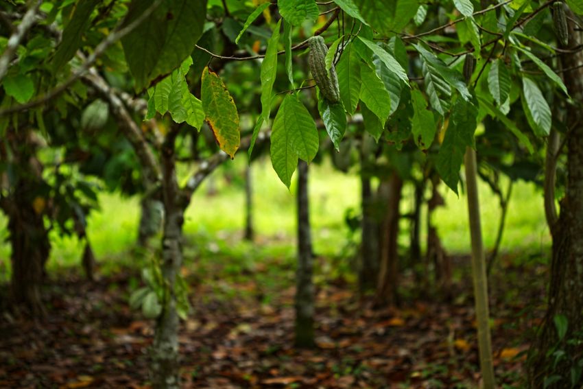
Project details
Project title   Quantification methodology and accounting framework for carbon
                sequestration in perennial cropping systems

Contracting     AM Fresh, Barry Callebaut, PepsiCo, Innocent, Mars, Mondelez, Nestlé,
organizations   Olam, Starbucks

Mission         The purpose of this report is to fill the knowledge gap regarding GHG
statement       accounting of carbon sequestration for perennial crops in order to
                provide the groundwork to answer: 1. What is the potential for perennial
                cropping systems to sequester carbon? 2. How can we develop a shared
                accounting methodology to help drive positive action? This report
                focuses on providing farm-level accounting methods for coffee, cocoa,
                apple, and citrus. The ultimate ambition is to use the best available
                scientific knowledge to shed light on the role of carbon removals in
                promoting sustainable perennial cropping systems. To apply the
                learnings and improve practice, additional funding and partners are
                invited to promote the integration of the methodology into geo
                Footprint and Cool Farm Tool and pilot the methodology.

Version         Final Report V1.0 January, 2022

                Alexi Ernstoff – PhD, Global science lead, Quantis
Project team    Alicia Ledo – PhD, Scientist & Environmental Consultant
                Daniella Malin - Deputy General Manager CFA
                Patrick Lawrence - PhD, Agricultural Systems and Sustainability
                Consultant, Repliculture LLC
                Paula Sanginés de Cárcer – PhD, Sustainability Consultant & Scientist
                in Forestry Sustainability, Quantis
                Richard Heathcote – CFA advisor and Sustainability Consultant

                                                                                           2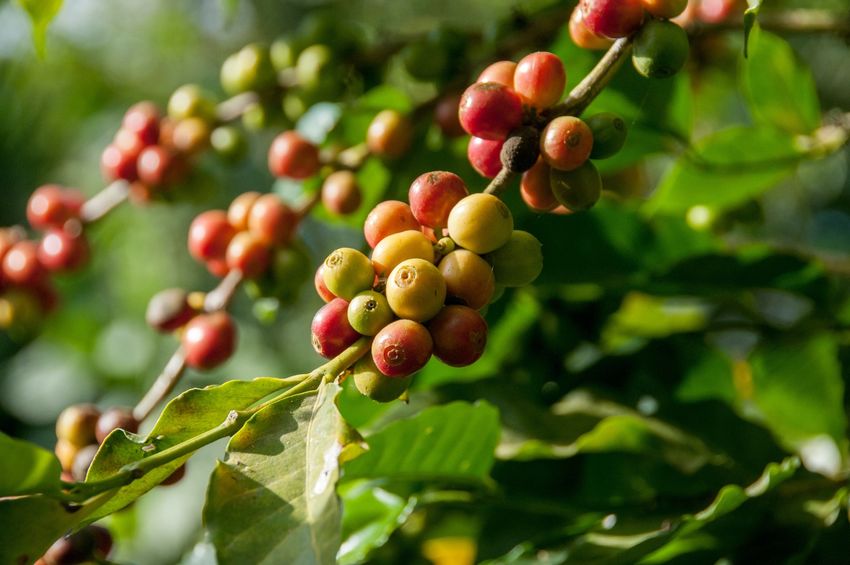
Acknowledgements
This methodology report is the result of the "Carbon sequestration in perennials" project
led by Cool Farm Alliance (www.coolfarmtool.org) and Quantis (www.quantis-intl.com)
and funded by:

We are grateful to the following people that gave valuable inputs to develop the
methodology through several exchanges and discussions:
   ●   Hans van Dieijen (Control Union)
   ●   Starry Sprenkle-Hyppolite (Conservation International)
   ●   Michiel Kuit (Agrilogic)
   ●   Eric Rahn (Alliance of Biodiversity International and CIAT)
   ●   Vern Long (World Coffee Research)
   ●   Maud Nicolas (World Coffee Research)
   ●   Prof. Rattan Lal (Ohio State University)
   ●   Barry Flaming (USAID)
   ●   Candace Vinke (Verra)

                                                                                            3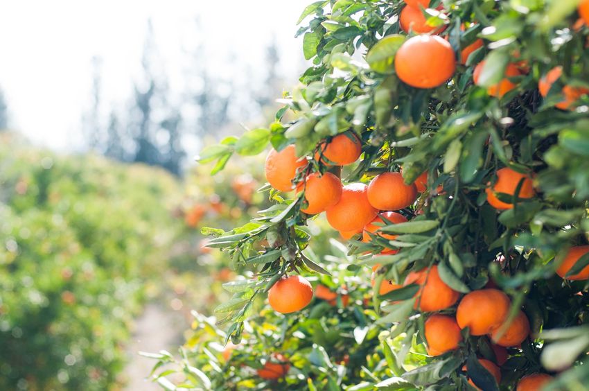
Disclaimer + use
Anyone is free to use and cite this methodological guidance for quantifying carbon
sequestration in perennial crops, namely cocoa, coffee, apple and citrus. Cool Farm
Alliance, Quantis, their associates and the funding partners cannot be held responsible for
any action or decision referencing these guidelines.
Generally, it is recommended that:
   ● All decisions consider multiple indicators (e.g. biodiversity, water, social metrics)
     and the potential for unintended consequences.
   ● Carbon sequestration is only reported when there has been a change in practice or
     management.
   ● Carbon sequestration is reported as the difference between two land management
     or land use scenarios. For perennial systems, an estimated (projected) average
     sequestration across a planting cycle is more appropriate than reporting year-by-
     year growth.
   ● The inherent reversibility of carbon sequestration in perennial systems is explicitly
     considered in assessment, communication, and monitoring.

Recommended citation: CFA & Quantis (2022). Quantification methodology and
accounting framework for carbon sequestration in perennial cropping systems.

                                                                                          4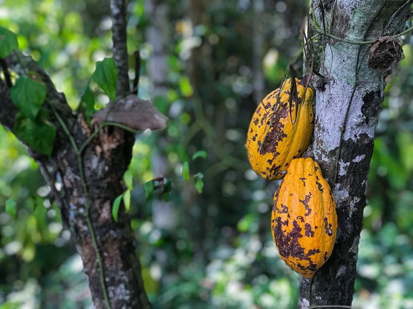
Table of contents
List of Figures .............................................................................................................................6
Glossary ......................................................................................................................................8
Summary ..................................................................................................................................10
1.      Introduction ......................................................................................................................12
     1.1.       Context .....................................................................................................................12
     1.2.       Objectives .................................................................................................................13
     1.3.       Method overview......................................................................................................14
2.      Inventory estimation ........................................................................................................16
     2.1.       Stoichiometric CO2 estimation ................................................................................16
     2.2.       Residue management ..............................................................................................16
3.      Estimating biomass ..........................................................................................................19
     3.1 Apple ...............................................................................................................................21
     3.2 Citrus ...............................................................................................................................23
     3.3. Cocoa .............................................................................................................................25
     3.4 Coffee ..............................................................................................................................28
     3.5 Shade trees, intercrops, and other perennial biomass ................................................30
4.      GHG accounting in CO2e ...................................................................................................34
     4.1.       Requirement of a reference state for accounting removals ..................................37
     4.2.       Carbon dioxide equivalents (CO2e) for removals ...................................................37
5.      Applicability and outlook .................................................................................................40
     5.1.       Applicability .............................................................................................................40
     5.2.       Future outlook .........................................................................................................40
A.1 Summary allometric equations developed in this study and respective carbon
fractions....................................................................................................................................47
A.2 References from literature review.....................................................................................50
        A.2.1 References used for Apple .......................................................................................50
        A.2.2 References used for Citrus ......................................................................................53
        A.2.3 References used for Cocoa ......................................................................................58
        A.2.4 References used for Coffee......................................................................................65

                                                                                                                                               5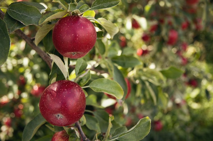
List of figures
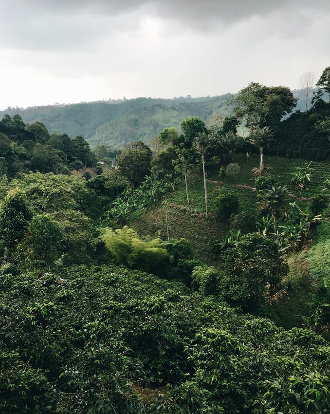
Figure 1. Typology illustration Example of how typology can influence allometry, i.e.
differences in tree shape and biomass accumulation can be expected when apple trees are
growing in different systems, e.g. wire-pole support (left) and traditional orchard without
support (right). Source: unsplash (left) .................................................................................. 19
Figure 2A-B. Apple Generic model as a function of age (year) fit for an individual apple
tree; A. (left) woody above ground biomass (AGB), which includes biomass in branches
and the main stem (RMSE = 11.8 kg), and B. (right) below ground biomass (BGB), which
includes the coarse and fine root (RMSE = 2.3 kg). ................................................................ 22
Figure 3A-B. Citrus Generic model parameterized as a function of age (year) for an
individual citrus tree; A. (left) woody above ground biomass (AGB), which includes
biomass in branches and the main stem (RMSE = 5.4), and B. (right) below ground biomass
(BGB), which includes the coarse and fine roots (RMSE = 0.9). ............................................. 24
Figure 4A-B. Cocoa high density Generic model parameterized as a function of age (year)
for an individual cocoa tree grown in a high density system; A. (left) woody above ground
biomass AGB, which includes biomass in branches and the main stem (RMSE = 11.9), and
B. (right) below ground biomass (BGB), which includes course and fine roots (RMSE = 8.7).
Cocoa high density has low accuracy especially for trees older than 15 years due to a
lack of sufficient primary data to fit the curve. ................................................................ 26
Figure 5A-B. Cocoa low density Generic model parametrized as a function of age (year)
for an individual cocoa tree grown in a low density system; A. (left) woody above ground
biomass (AGB), which includes biomass in branches and the main stem (RMSE = 31.8), and
B. (right) below ground biomass (BGB), which includes the coarse and fine roots (RMSE =
2.1). .......................................................................................................................................... 27
Figure 6A-B. Coffee monoculture Generic model parametrized as a function of age (year)
for an individual coffee tree grown as monoculture (no shade); A. (left) woody above
ground biomass (AGB), which includes biomass in branches and the main stem (RMSE =
2.38), and B. (right) below ground biomass (BGB), which includes the coarse and fine roots
(RMSE = 2.89). .......................................................................................................................... 29
Figure 7A-B. Coffee agroforestry Generic model parametrized as a function of age (year)
for an individual coffee tree grown in an agroforestry system (with shade); A. (left) woody
above ground biomass (AGB) which includes biomass in branches and the main stem
(RMSE = 5.88 kg), and B. (right) below ground biomass (BGB), which includes the coarse
and fine roots (RMSE = 2.43). A high uncertainty of the AGB estimation is present for
trees older than 20 years. ..................................................................................................... 30
Figure 8. Average stock over a cycle period is the area under the growth curve (i.e.
cumulative growth in a year * 1 year) divided over the cycle length including years of fallow.
.................................................................................................................................................. 35
6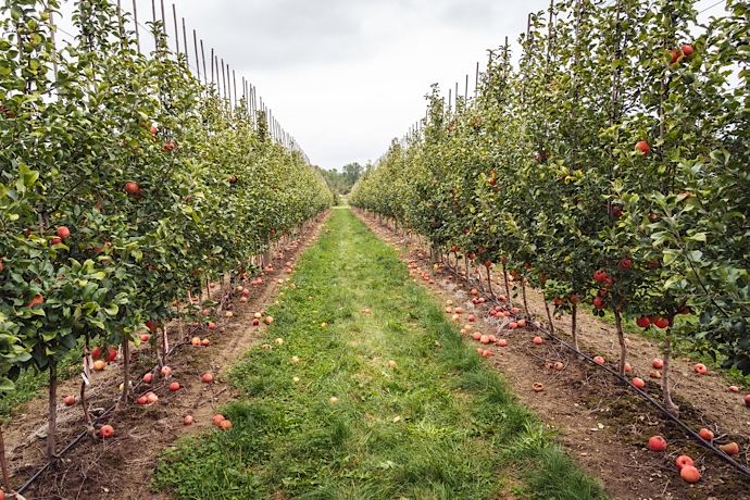
List of tables
Table 1. Allometric equations for shade trees, intercrops and hedges, where the age of the
tree in years and the diameter at breast height (DBH) can be used to estimate the biomass
(B) in kilograms per tree, the above ground biomass (ABG) in kilograms per tree, or the dry
matter (DM). fC_biomass is the fraction of molecular carbon in biomass. .................................. 30
Table A2. Allometric equations for individual trees, where AGBwoody= Woody above ground
biomass (kg/tree) including branches and stem; BGB = Below ground biomass for course
and fine roots (kg/tree); age (years); LEAF = leaf biomass (kg/tree); RMSE = root-mean-
square error. The allometric equations are valid within the given age range...................... 47
Table A3. fC_biomass, carbon (C) fraction in biomass. ................................................................ 49

                                                                                                                       7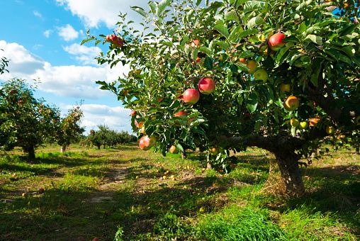
Glossary
Allometric equation: A mathematical expression describing the shape of trees due to
growth through time by relating a dependent variable (e.g. tree biomass) with measurable
independent variables (e.g. tree diameter at breast height, age and height).
Biomass: The material of living plant parts containing organic carbon and generally
expressed in kilograms (kg).
Carbon dioxide: A greenhouse gas molecule consisting of one carbon (C) and two oxygen
(O) atoms (CO2) with the molecular weight of 44 g/mol.
Carbon dioxide removal: The process of capturing CO2 from the atmosphere and storing it
in material form as organic or inorganic carbon.
Carbon sequestration: The process by which CO2 is removed from the atmosphere and
stored in organic stocks (e.g. soil and tree biomass).
Carbon stock: The amount of carbon in a carbon pool, i.e. a reservoir in an earth system,
often expressed as tonnes per hectare (t/ha).
Climate benefit: A climate benefit in this methodology refers to a removal of CO2 expressed
as a negative emission of CO2, while acknowledging that removals associated with any
given system may not influence global climate.
Climate impact: A climate impact refers to GHG emission, while acknowledging that
emissions for any given system may not influence global climate.
Carbon dioxide equivalent (CO2e): Equivalency of carbon dioxide (CO2e) is the quantity of
CO2 emission that would cause the same integrated radiative forcing over a given time
horizon, as an emitted amount of greenhouse gas. For various greenhouse gases this value
is obtained by multiplying the emission of a gas by the global warming potential for that
gas, referred to as a characterization factor in life cycle assessment. For removals, CO2e is
used to express the equivalent amount of CO2 removal (considering mass and time period)
that would be needed to neutralize an emission considering global warming potential 100
(GWP 100). This value is not the same as stoichiometric CO2 which represents the amount
of carbon in biomass at any given moment, and not the influence on climate over a time
horizon. Equivalent carbon dioxide emission is a common scale for comparing emissions of
different greenhouse gases but does not imply equivalence of the corresponding climate
change responses over various timescales according to the IPCC.
Diameter at Breast Height (DBH): A tree trunk’s diameter at 1.3 m above the ground.
Global warming potential (GWP): The GWP is defined as the ratio of the time-integrated
radiative forcing from the instantaneous release of 1 kg of a substance relative to that of
1 kg of a reference gas, where the conventional reference gas in greenhouse gas

                                                                                              8
accounting is CO2, and the time horizon is 100 years. By definition, the GWP of an emission
of CO2 is 1.

Growth model: A mathematical expression that relates easy-measurable variables (e.g.
tree age, DBH, height) with biomass.
Land management change (LMC): A change in land management that occurs within a land
use category. Management is a generic term for anthropogenic influence on land and
encompasses a wide variety of practices.
Land use: The total of arrangements, activities and inputs applied to a parcel of land. Land
use is classified according to the IPCC land use categories of forest land, cropland (annual
and perennial), grassland, wetlands, settlements, other lands.
Land-use change (LUC): The change from one land use category to another.
Neutralization potential: The indicator of negative carbon dioxide equivalents (-CO2e) and
the value that can be considered to neutralize emissions from sequestration.
Responsibility window: The time period the system under consideration is responsible for
carrying the impacts or benefits of gains and losses of sequestered carbon. The
responsibility window determines the reference state and the total relevant inventory for
an assessment year. In land-use change accounting this is referred to as the “look back
period” or the “amortization period,” which are typically equal in time period.
Reference state: The reference state is the stock quantity in units of stoichiometric CO2 per
land area to which cumulative changes in net stock are considered. The reference state is
defined as the stock amount just before the initiation of the responsibility window.
Stoichiometric CO2: Organic carbon (C) stocks within soils or biomass, that’s origin is from
atmospheric CO2 formed into biomass through photosynthesis, expressed in units CO2 by
adjusting the molecular weight ratio of CO2 to carbon (C) 44:12. This metric is not the same
as CO2e, which implies the influence on climate over a time horizon.
Stored CO2: In this guidance, stored CO2 refers to the C sequestered in stocks that keep CO2
out of the atmosphere and in a carbon stock for a period of time.
Perennial crop: Crops that – unlike annual and biennial crops – do not need to be replanted
each year or every two years.
Typology: A distinctive growth pattern of a tree/plant resulting from the combination of
factors such as type of species, variety, growing conditions and management practices.

                                                                                            9
Summary
Recent consensus science (IPCC, 2021) emphasizes that, to avoid extreme impacts of
climate change, large-scale and long-standing removal of atmospheric CO2 is essential
to neutralize residual greenhouse gas (GHG) emissions that cannot be feasibly reduced.
Most current methods and tools for product and corporate GHG accounting, however,
exclude the influence of land-based GHG emissions and CO2 removals.
To address this methodological gap, track progress and improve decision-making, one key
need is to understand the amount of carbon able to be removed from the atmosphere
through photosynthesis and sequestered by perennial crop farms. Recent work (Ledo et
al. 2018, 2020) has improved modelling of carbon sequestered by perennial plant biomass
above and below ground. A second major need is to be able to indicate emitted and
removed carbon dioxide equivalents (CO2e), a metric relevant for GHG accounting that
considers the atmosphere over a time horizon. In the case of sequestered carbon, the
concept of neutralization potential (-CO2e) is presented. Recent draft guidance for carbon
sequestration has been presented (Quantis, 2021) but, at the time of preparing this report,
there are no widely accepted methods for GHG accounting of carbon sequestration.
This work aimed to fill the methodological gap in current GHG accounting of carbon
sequestration and emissions associated with perennial biomass by developing a common
public methodology. A detailed literature review and stakeholder engagement phase
gathered available data on biomass measurements from previous destructive sampling for
apple, citrus, cocoa and coffee trees. A procedure then follows to fit a model to these
measurements and ultimately indicate neutralization potential (-CO2e) of carbon
sequestered in perennial systems. Neutralization potential is only valid if a land
management or practice change occurs that leads to additional carbon sequestration
(i.e. the difference between a reference state and a new, improved state). The methodology
also considers future reversibility of carbon sequestered in perennial systems (e.g. due to
planting cycles or unexpected events such as fires).
This work demonstrated insufficient measurements to accurately fit models for various
perennial crops. This indicates a need for future data-driven refinement and alternative
methods, such as remote sensing, and agreement on the needed accuracy of carbon
sequestration estimation for product and corporate GHG accounting. Further work, for
example, a digital tool and monitoring is needed to pilot this methodology and ground-
truth findings. Beyond sequestration’s influence on climate, it is always important to
consider other co-benefits and trade-offs (e.g. related to biodiversity, water, pest
management, and human labor) to support holistic decision-making for more resilient and
sustainable perennial cultivation systems.
1001
Introduction
111. Introduction
1.1. Context
The science presented by the Intergovernmental Panel on Climate Change (IPCC) indicates
a need to drastically reduce greenhouse gas (GHG) emissions to avoid extreme impacts of
climate change on human society (IPCC, 2021). There is increasing scientific evidence that,
when combined with deep GHG reductions, large-scale and long-standing removal of
carbon dioxide (CO2) from the atmosphere is necessary to neutralize remaining emissions
that cannot be feasibly reduced. With land-intensive sectors representing nearly a quarter
of global GHG emissions and, at the same time, having an opportunity to remove CO2
through carbon sequestration in soils and biomass, many companies in the food and
beverage industry are committing to targets to decrease emissions and remove CO2 from
the atmosphere, for example toward net-zero (SBTi, 2021). To set strategies and track
progress toward targets, science-based methods are needed to guide business action.
The science of carbon sequestration is increasingly understood, but at the time of
preparation of this report, common product footprinting practices such as the Publicly
Available Standard 2020:2011 (PAS2050), the EU Renewable Fuel Directive (RED) and the
GHG Protocol (ghgprotocol.org) do not consistently consider removals related to carbon
sequestration. There are two major scientific challenges that prevent consistent
accounting: one is estimating sequestered carbon in biomass and the other is accounting
for sequestered carbon in terms of CO2 equivalent (CO2e), which considers a gain from a
reference state and the length of time the CO2 is removed.
The process of carbon sequestration begins when organic carbon (C) is assimilated into
plants from atmospheric CO2 through photosynthesis, which removes CO2 from the
atmosphere and fixes it in biomass. Humans and nature can influence the fate of C in plant
biomass and whether it is re-emitted to the atmosphere as CO2 or CH4 (methane) or
sequestered over time. Deforestation, for example, through slash and burn practices to
prepare land for perennial cultivation, is an example of disturbing biomass and emitting
CO2. When performed at a large scale, increasing biomass stocks in agricultural systems, for
example through agroforestry, afforestation and reforestation, can remove CO2 from the
atmosphere (Roe et al., 2019, 2021). Various management practices that can increase
biomass stocks (e.g. the use of shade trees) over business as usual may also influence other
aspects of agricultural systems in relation to agrochemical inputs, biodiversity and human
labor (Clough et al., 2011). Improving decision-making related to perennial cultivation is an
opportunity to decrease emissions, increase removals and promote other benefits.
In addition to agroforestry, afforestation and reforestation, residue management can
12influence emissions and removals. Residue management can lead to carbon sequestration
in soils and/or can emit CO2, CH4 or N2O (nitrous oxide), which are more potent GHGs than
CO2. For instance, burning residues from pruning leads to emissions, whereas mulching
residues can potentially lead to soil carbon sequestration. Several research initiatives have
developed reliable methods to quantify crop biomass and the GHG accounting related to
its management (Ledo et al., 2018).
The estimation of fixed carbon in biomass as stoichiometric CO2 (i.e. the amount of CO2 that
was removed from the atmosphere, obtained by multiplying the amount of carbon in
biomass by the fixed stoichiometric ratio of molecular weights of CO2:C 44/12) is only one
need for GHG accounting. Other important needs are that the GHG accounting reflects only
additional carbon sequestration in comparison to a reference state and its storage time and
potential reversibility (release back to the atmosphere). Reversibility is especially
important for perennial systems which are typically planned to be removed when no longer
economical. To account for reversibility, there are a variety of approaches ranging from
ensuring permanence through monitoring or financial schemes (COWI, Ecologic Institute
and IEEP, 2021) to dynamic GHG accounting that considers the impacts on climate of
sequestering carbon temporarily and delaying re-emission to the atmosphere (Brandão &
Canals, 2013; Brandão et al., 2019; Levasseur & Miguel Brandão, 2012).
Time is a key consideration in GHG accounting. It is widely accepted (IPCC, 2021) that the
indicator for climate change is carbon dioxide equivalents (CO2e) using global warming
potential over a 100-year time horizon (GWP 100) of atmospheric behavior. Put simply,
using GWP 100, CO2 would need to be removed from the atmosphere for 100 years in
order to neutralize an equivalent CO2 emission into the atmosphere with respect to
accounting (EC-JRC-IES, 2010). Using CO2e obtained from GWP 100 is an accounting
convention to have a common scale for comparing and summing GHG flows (IPCC, 2013). If
CO2 is temporarily removed and likely to be released in the future, the accounting should
reflect this. As examples, if 1 tCO2 is known to be removed for 10 years, this could be
accounted for as -0.1 tCO2e (10%, or 10 out of 100 years). At the time of preparing this report,
there is no accepted convention for temporary CO2 removal and deriving neutralization
potential: the presented methods are thereby flexible and do not prescribe a single
approach.
1.2. Objectives
This project aims to fill the knowledge gap regarding accounting for carbon
sequestration in farm-level GHG assessments of perennial cropping systems.
To fill the methodological gap regarding GHG accounting of carbon sequestration in
perennial crops, AM FRESH, Barry Callebaut, innocent drinks, Mars, Mondelēz, Nestlé, Olam,
13PepsiCo and Starbucks launched this work with Quantis, the Cool Farm Alliance and Control
Union. This work aimed to establish an operational methodology and framework among
different stakeholders. The methodology is not intended to cover emissions from perennial
crop systems that are already covered by existing methods (for example, from fertilizer or
fuel use) (Hillier et al., 2011; Kayatz et al., 2020; Nemecek., 2019). Rather, it focuses on
emissions and removals related to perennial biomass.
This publicly available methodology provides a common framework to explore how
agricultural practices can influence the emissions and sequestration of organic carbon in
perennial systems, focusing on apple, citrus, cocoa and coffee. The ultimate aim is that
the methodology presented can supplement existing footprinting tools such as the Cool
Farm Tool and geoFootprint.
Further funding will be required to improve the methodology, for example by collecting
primary data to refine the typology parameterization and to digitalize the methodology into
a user-friendly tool. To apply the learnings and improve practice, funding and partners are
invited to promote the integration of this methodology into geoFootprint and the Cool Farm
Tool, and pilot the methodology.
1.3. Methodology overview
The methodology presented in this document includes:
• Carbon accumulation in perennial biomass, both above and below ground, as a
function of time. Quantification of biomass is achieved via growth models that have
been parameterized from primary, empirical data from literature.
• The carbon stored in the biomass is subsequently converted into stoichiometric
carbon dioxide (CO2) “stock” by the molecular weight ratio of CO2:C 44/12.
• Plant residue (e.g., from pruning) management (e.g., composting) is accounted for.
• Neutralization potential as negative carbon dioxide equivalents (-CO2e) is indicated
considering the average stock over a perennial cycle, the difference between a
reference or baseline system stock and the system following a land management
change, and the global warming potential over a 100-year time horizon (GWP 100).
1402
Inventory Estimation
152. Inventory estimation
The inventory (amount of) emission and sequestration as a result of the management of
biomass in perennial crops, shade trees, intercrops and other trees, is a key piece of this
methodology. This framework fills a major knowledge gap in current GHG accounting of
perennial systems and can complement existing methods to quantify GHG emissions due
to farm management.
2.1. Stoichiometric CO2 estimation
The term "stoichiometric" refers to the molecular ratio between CO2 and C (44/12), and
is conceptually different from carbon dioxide equivalents (CO2e). CO2e is characterized
inventory that considers a time horizon for the influence on the atmosphere (more
information in section 4). Estimating the amount of stoichiometric CO2 in a tree is an
important first step in creating an inventory to estimate further emission of carbon
molecules (CO2 and CH4) and carbon sequestration (-CO2).
To estimate the kilograms of stoichiometric CO2 removed from the atmosphere for the trees
in a perennial system the following equation can be used:
..
!"!_#$%&'(&%)*$+&' = $ ∗ &$+**, ∗ '-!"#$%&& ∗ /! Equation 1
Where:
• B is the biomass estimated by the individual based model (IBM) according to the
typology (section 3) and in terms of kilograms per tree, see appendix table A.2.
• ntrees is the number of trees being considered of the same typology of the individual
based model, for example per hectare.
• fC_biomass is the carbon (C) fraction in biomass, see appendix table A.3.
• 44:12 is the stoichiometric ratio of molecular weight of CO2:C.
2.2. Residue management
Residues are a key part of estimating emissions (and sequestration) from perennial
systems. Residues can lead to release of biogenic CO2, CH4, N2O. The individual-based model
that estimates perennial biomass is also useful to estimate plant residues. Residues are
any perennial biomass removed naturally or by management. Any plant part can
become residue; for example, leaves and roots die and become residues, branches are
pruned and become residues. Plant parts that can be managed are distinguished as litter
and leaves, pruned material, trees that die prematurely, woody material at the end of a
16cropping cycle, unsuitable fruit, and fruit pulp (Schulze and Freibauer, 2005, Wu et al. 2012,
Ledo et al., 2018). Roots are also considered as a source of residue but are not considered
in this method framework to be “manageable”; coarse roots are assumed to remain intact
during the tree lifetime whereas fine roots and are assumed to die and grow back every year
and either decompose to emit biogenic CO2 or add to the SOC pool (Aber et al. 1990;
Withington et al., 2006). By and large, 98% of fine roots will decompose within few years
and the model incorporates decomposition for fine roots during cultivation period.
The fate of managed residues included in the modeling framework include:
• Burning (Akagi et al., 2011)
• Spreading on soil (Liski et al., 2005, Weedon et al. 2009)
• Removing outside the farm boundary (considered out of the system boundary, and set
to “0” emission and sequestration)
• Composting: two main technologies, open and close compost, for woody parts, litter
and unsuitable fruits or parts of the fruit (Boldrin et al. 2009)
Wet residue management was not included in the modeling framework as it is considered
a processing step which is out of the system boundaries covered in this farm-level
methodology.
1703
Estimating biomass
183. Estimating biomass
This project parameterizes a generic model (Ledo et al., 2018) in order to estimate biomass
accumulation for commercially relevant perennial typologies for apple, citrus, cocoa, and
coffee (e.g. coffee robusta growing under shade in Vietnam). A typology is the combination
of crop, variety, growing system, agronomy and geography that defines an allometric
(shape) curve. Each typology has a different growth pattern and biomass accumulation
reflected in the allometric curve fitted to empirical data.
Figure 1. Typology illustration Example of how typology can influence allometry, i.e. differences in tree shape and
biomass accumulation can be expected when apple trees are growing in different systems, e.g. wire-pole support (left)
and traditional orchard without support (right). Source: unsplash (left)
It is generally known that naturally trees follow a sigmoid shape growing curve, meaning
that older trees decelerate the rate of biomass increase. However, this shape has not been
observed in empirical data on perennial crops (Ledo et al., 2018). This is likely because
typical crop cycles maximise productivity and are not long enough to observe the
deceleration in biomass. In other words, perennial crop trees rarely reach their “natural”
end-of-life since trees are replaced once the optimal yield production decreases. Using
different functions to model empirical data on perennial crops, it has been observed that
the power law function (not a sigmoidal function) provided the best fit, and is
mathematically simple (Stephenson et al., 2014).
The generic individual-based model (IBM) growth model for estimating biomass (B) is
therefore a power law function with the form of:
$ = ) *+, 0 Equation 2
where the parameters ) and - define the shape of the growth according to the typology,
and age is the independent variable. The required empirical data for model
parameterization are the biomass quantity of the different plant parts at different ages. For
every case, curves were fitted to estimate above and below ground biomass separately as
19a function of age. Also leaf biomass was estimated as a function of branches and crown size.
The accuracy of the parameterized model is mainly dependent on the quality and quantity
of the primary data available. Primary data in this case require destructive sampling (i.e.
killing of trees) to obtain the mass of biomass at each age. Parameter estimation was done
using nonlinear least-squares estimate fit to empirical data. The better the parametrization
and lower the Root Mean Square Error (RMSE), the better the fit of the model.
Appendix A.1 includes a summary of all allometric equations developed in this study.
Each typology and its parameterization is described below.
203.1 Apple
©Unsplash
Apples are one of the most valuable fruit crops in temperate regions. Apples are grown for
three main purposes: produce, juice production (juicing), and cider making. Produce and
juicing apples are traditionally grown on semi-dwarfing rootstock to allow for hand picking,
and are now increasingly grown on smaller root stocks on a post and wire system, at higher
densities. Cider apples (which have higher tannin content) are grown as 'bush orchards' on
semi-dwarfing root stocks and have a different pruning regime, and globally represent a
small proportion of all apples with production concentrated in regions of UK, Spain, and
France. China is the largest global producer of apples, mainly for concentrate juice
production (Wu et al., 2012).
21All biomass data retrieved from literature review were related to traditional growing
systems. Data for modern wire & pole systems were not found. Several studies showed
differences in biomass due to pruning regimes and rootstock. There was insufficient data,
however, to observe significant differences in pruning regimes and rootstock along with
other variables.
Following an extensive literature review and stakeholder consultation, data
were sufficient to parameterize:
- A single typology for apple orchards
Figure 2A-B. demonstrates the parameterization of above and below ground biomass for
apple.
Figure 2A-B. Apple Generic model as a function of age (year) fit for an individual apple tree; A. (left) woody above ground
biomass (AGB), which includes biomass in branches and the main stem (RMSE = 11.8 kg), and B. (right) below ground
biomass (BGB), which includes the coarse and fine root (RMSE = 2.3 kg).
223.2 Citrus
©Unsplash
Citrus includes oranges, mandarins, lemons, limes, grapefruits and citrons. Citrus is
cultivated in many regions of the world and is used mainly as edible fruit or juice. The
main producers are China, Brazil, USA and Spain (Pérez-Piqueres et al., 2019).
Commercial citrus is generally cultivated in monocultures and the main factor affecting
its growth pattern is the grafting methodology. It has been observed that different
rootstock sources and sions lead to different yields and biomass and are therefore a
major commercial consideration (Mourão Filho et al., 2007).
23Pruning is one of the key factors affecting citrus biomass, however there were insufficient
data to parameterize according to different pruning regimes. The effect of varieties, regions
and rootstock was also analysed; however, the lack of data did not allow to differentiate
typologies robustly.
Following an extensive literature review and stakeholder consultation, data were
sufficient to parameterize:
● A single typology for citrus orchards
Figure 3A-B. demonstrates the parameterization of above and below ground biomass for
citrus.
Figure 3A-B. Citrus Generic model parameterized as a function of age (year) for an individual citrus tree; A. (left)
woody above ground biomass (AGB), which includes biomass in branches and the main stem (RMSE = 5.4), and B. (right)
below ground biomass (BGB), which includes the coarse and fine roots (RMSE = 0.9).
243.3. Cocoa
©Unsplash
Cocoa (Theobroma cacao L.) is an important soft commodity worldwide, producing 5.3
million tonnes of dry beans in 2018 mostly by small holders in African countries (Neither
et al., 2020). Cocoa cultivation has been intensified where shade systems have been
gradually replaced with full-sun monocultures and the use of agrochemicals (Neither et
al., 2020). In addition to improving yield (with shade up to 30%), shade cultivation can
have added benefits related to biodiversity, diversity in income, and more resiliency to
climate change and pests (Blaser et al., 2018; UTZ, 2017).
25Cocoa biomass accumulation is affected by shade gradients, where yields can decrease
above 30% shade (UTZ, 2017), nutrient inputs through fertilizer, and climate zone. Shade
coverage ranges from intensive management with cacao-monoculture with high densities,
intermediate management with monospecific shade trees (legume-cocoa; timber species-
cocoa; rubber-cocoa), and extensive management with higher diversity of species and lower
cocoa densities. Data were sufficient to consider high and low density cocoa typologies;
however, for high density cocoa there were limited data above age 15 which should be
considered when interpreting results.
Following an extensive literature review and stakeholder consultation, data
were sufficient to parameterize:
- High density cocoa (> 1000 cocoa trees/ha)
- Low density cocoa (< 1000 cocoa trees/ha)
Figure 4-5A-B demonstrate the parameterization of above and below ground biomass for
cocoa.
Figure 4A-B. Cocoa high density Generic model parameterized as a function of age (year) for an individual cocoa tree
grown in a high density system; A. (left) woody above ground biomass AGB, which includes biomass in branches and the
main stem (RMSE = 11.9), and B. (right) below ground biomass (BGB), which includes course and fine roots (RMSE = 8.7).
Cocoa high density has low accuracy especially for trees older than 15 years due to a lack of sufficient primary data
to fit the curve.
26Figure 5A-B. Cocoa low density Generic model parametrized as a function of age (year) for an individual cocoa tree
grown in a low density system; A. (left) woody above ground biomass (AGB), which includes biomass in branches and the
main stem (RMSE = 31.8), and B. (right) below ground biomass (BGB), which includes the coarse and fine roots (RMSE = 2.1).
273.4 Coffee
©Unsplash
Coffee is a soft commodity with two main varieties covering 95% of the market:
arabica (Coffea arabica L.) and robusta (Coffea canephora L.). Arabica (which has
higher trade volumes than robusta) is commonly grown at higher elevations (between
1000 and 2500 m) than robusta (between 200 and 800 m). Coffee is a shade-tolerant
crop which is commonly grown in the understory. In spite of the multiple benefits of
coffee grown in agroforestry, in the recent decades there has been a global
transformation of coffee production into more intensified systems by removing shade
trees and increasing chemical fertilizations (Jezeer & Verweij, 2015).
28Coffee biomass accumulation is affected by shade gradients, variety (robusta and arabica),
nutrient inputs through fertilizer, and climate zone (Piato et al., 2020; Rodriguez 2011).
Similar to cocoa, there is an optimal shade coverage that is approximately 30% (UTZ, 2017).
The degree of shading and the degree of management are generally related where the more
intense management are often monoculture with no shading while more extensive
management through agroforestry has higher canopy shade. Shaded and unshaded coffee
had sufficient data for parameterization; however, there were a lack of sufficient empirical
data above age 20, which should be considered when interpreting results.
Following an extensive literature review and stakeholder consultation, data
were sufficient to parameterize:
- Coffee monoculture
- Coffee agroforestry
Figure 6-7A-B demonstrate the parameterization of above and below ground biomass for
coffee.
Figure 6A-B. Coffee monoculture Generic model parametrized as a function of age (year) for an individual coffee tree
grown as monoculture (no shade); A. (left) woody above ground biomass (AGB), which includes biomass in branches and the
main stem (RMSE = 2.38), and B. (right) below ground biomass (BGB), which includes the coarse and fine roots (RMSE = 2.89).
29Figure 7A-B. Coffee agroforestry Generic model parametrized as a function of age (year) for an individual coffee tree
grown in an agroforestry system (with shade); A. (left) woody above ground biomass (AGB) which includes biomass in
branches and the main stem (RMSE = 5.88 kg), and B. (right) below ground biomass (BGB), which includes the coarse and
fine roots (RMSE = 2.43). A high uncertainty of the AGB estimation is present for trees older than 20 years.
3.5 Shade trees, intercrops, and other
perennial biomass
Woody plants in the cultivated area that are not the main crop, namely shade trees, trees in
agroforestry systems, hedgerows and other perennial intercrops are generally referred to
as out of crop biomass (OOCB). To estimate OOCB published allometric equations were
used or empirical data was used to parametrize the generic allometric model. Perennial
grasses and non-woody crops were not covered in the current modeling approach.
The most common intercrop species (e.g. found in coffee and cocoa agroforestry systems)
were considered and the corresponding equations are presented in Table 1. To estimate
the C accumulated in hedgerows, values of AGB of the individuals for each species were run
using allometric equations from literature and considering a default age of 20 years.
Table 1. Allometric equations for shade trees, intercrops and hedges, where the age of the tree in years and
the diameter at breast height (DBH) can be used to estimate the biomass (B) in kilograms per tree, the above
ground biomass (ABG) in kilograms per tree, or the dry matter (DM). fC_biomass is the fraction of molecular
carbon in biomass.
Shade tree/Intercrop Allometric equation fC_biomass Source
Tropical shade trees in wet 0.45 Fitted in this study
areas (Canopy trees) ! = 0.344'() ! − 0.6043'() + 1.5602
Tropical shade trees in wet 0.45 Fitted in this study
areas (understory) ! = 0.1212'() ! − 0.0317'() + 0.1853
30Tropical shade trees in dry 0.5 Fitted in this study
areas ! = −0.0065'() ! + 0.7165'() + 1.1337
Temperate conifers 0.4 Fitted in this study
! = −0.0485'() ! + 7.3469'() − 12.712
Temperate broadleaf trees 0.4 Fitted in this study
! = 0.8101'() ! − 6.6956'() + 21.651
Temperate shrubs 0.45 Fitted in this study
! = −0.0099'() ! + 1.2424'() − 1.4514
Intercrop avocado (Persea 0.4 Kuit et al., 2020
americana Mill.) 34! = 2.7856'() ".$%&'
Intercrop cashew (Anacardium 0.4 Kuit et al., 2020
occidentale L. ) 34! = 43.807 '() %.(")!
Intercrop durian (Durio 0.4 Kuit et al., 2020
zibetinus L.) 34! = 3.2868 '() ".$&))
Intercrop jackfruit (Artocarpus 0.4 Kuit et al., 2020
heterophyllus Lam.) 34! = 0.0939 '() ).%*!'
Intercrup rubber (Hevea 0.4 Kuit et al., 2020
brasiliensis Müll.Arg.) 34! = 11.699 '() "."'$&
Intercrop other perennial 0.4 Ledo et al., 2018
woody species 34! = 1.5 '() ".")
Hedge ash (Fraxinus sp.) 0.4 Fitted in this study – using
Bage=20= 96.4 allomeric curves from
AGB = 0.085 × DBH2.4882 Lingner et al., 2018 and
growth from Yoshimoto et
al., 2007
Hedge maple (Acer sp.) 0.4 Fitted in this study – using
allomeric curves from
Bage=20 = 96.3 Lingner et al., 2018 and
DM = 0.067 × DBH2.5751 growth from Yoshimoto et
al., 2007
Hedge oak (Quercus sp.) 0.47 Fitted in this study – using
allomeric curves from
Bage=20 = 95.6 Lingner et al., 2018 and
DM = 0.089 × DBH2.4682 growth from Yoshimoto et
al., 2007
31Hedge poplar (Populus sp.) 0.3 Fitted in this study – using
allomeric curves from
Bage=20 = 96.5 Lingner et al., 2018 and
DM = 0.089 × DBH2.4682 growth from Yoshimoto et
al., 2007
Hedge (mixed-species & other 0.4 Fitted in this study – using
broadleaf) allomeric curves from
Bage=20 = 96 Lingner et al., 2018 and
growth from Yoshimoto et
al., 2007
3204
GHG accounting in -CO2e
334. GHG accounting in -CO2e
The overall framework for GHG accounting of the neutralization potential (-CO2e) of carbon
sequestration goes beyond the simple estimation of yearly carbon in biomass and its
multiplication by the stoichiometric ratio of CO2:C 44/12 (Equation 1). The GHG accounting
of neutralization potential must consider only additional increases in carbon stocks; for
example, the difference between the average stock in a new system following a land
management change and the average stock in a prior reference system (section 4.1-4.2).
Further, GHG accounting should also consider that sequestered carbon can be reversed
and thus the benefits on climate may not be long-standing. This means the neutralization
benefits of future removal should not be concentrated into a single accounting year, but
spread over a responsibility window (section 4.2). This is true for perennial cycles also when
assuming a permanent change to a new system and thus a permanent sequestration
of additional carbon stock, because in order for the change to be fully realized there needs
to be a full cycle.
Boxes 1-4 demonstrate the overall framework, according to the following steps
• Quantify the amount of biomass in individual trees (Box 1)
• Quantify the amount of stoichiometric CO2 stocked on average over a planting cycle
for the two systems in consideration (i.e. the reference system and the new system
following a land management change) (Box 2)
• Quantify the difference in the stocked stoichiometric CO2 in the two system (Box 3)
• Quantify the final CO2 that can be accounted for in a GHG assessment (Box 4)
4.1. Average stock over a cycle
Because perennial systems are cycling and trees grow through time and then are planned
to be removed and re-planted, it is not recommended to consider yearly growth of trees in
product and corporate footprinting, and instead to consider an anticipated average stock
over a perennial life cycle. The gain in average stock between two systems should be spread
over a cycle length which includes years of fallow (i.e. years without trees), and includes
mortality and pruning and other aspects that may influence stock each year.
An example of how to compute a stock average over a cycle is provided using a linear
growth curve in figure 8. In this example, a yearly accumulation of biomass in an area is 100
kg CO2/year and the trees are planned to be planted, removed, and re-planted in 8-year
cycles with 2 years of fallow in-between planting. In practice, when estimating an intensity
(i.e., per kg of crop product) the area under the curve (the sum of each year’s cumulative
stoichiometric CO2 stocked) can be divided by the cumulative yield produced over the
34entire cycle. Given the example in figure 8, if there was a hypothetical yield of 80 t/ha-y and
thus 800 t of crop product produced through the years of the cycle, the intensity would be
the area under the curve 3,200 kg CO2*y divided by 800 t or 4 kg CO2-year/ t of product. This
unit represents the per product allocation of carbon dioxide that has been
photosynthesized into biomass and kept out of the atmosphere over a year of time.
Area under the curve Cycle length
800 ∗ 8 1
∗ = 320 *+ ,-!_#$%&'(&%)*$+&'
2 8+2
*+ ,-!_#$%&'(&%)*$+&'
max
800
average
fallow
8 10
Years
Figure 8. Average stock over a cycle period is the area under the growth curve (i.e. sum of annual cumulative
growth * 1 year) divided over the cycle length including years of fallow.
35Box 1: Quantify the amount of biomass in individual trees.
Obtain the kilograms of
!" 2345677
biomass stocked in individual
89++
trees over their lifetime using
an allometric growth model.
Years
Box 2: Quantify the amount of stoichiometric CO2 on average stocked over a planting cycle for two systems.
51 7&%)/## 51 , 88 51 ,-"
&,-!_._/01 [!" #$!_#$%&'(&%)*$+&' ] = =/01 [ ] ∗ >$+** [89++] ∗ :,! [ ] ∗ [ ]
$+** 51 7&%)/## 9! 51 ,
System A System B
Obtain the average increase in stocked (reference) (change)
biomass in terms of stoichiometric CO2
over a planting cycle for the system(s) Cycle 1
(&,-!_._/01 ). This is a function of the
!" #$!_#$%&'(&%)*$+&'
average biomass accumulated in trees
over the planting cycle (Bavg), the Cycle 1
number of trees (ntree), the fraction of Average
carbon in biomass (:,! ), and the
stoichiometric adjustment of the Average
molecular weight ratio of CO2 to C
(44/12).
Years
Box 3: Quantify the difference in stocked stoichiometric CO2 on average for two systems.
Obtain the difference in the carbon stocked in the reference system System A System B
!"#$!_#$%&'(&%)*$+&'
and the new system following a land management change. (reference) (change)
∆&,-!_._/01
∆&,-!_._/01 !" #$!_#$%&'(&%)*$+&' = &,-!_._/01_23#$*)_4 − &,-!_._/01_23#$*)_.
Box 4: Quantify the neutralization potential of sequestered carbon that can be accounted for in a GHG assessment
The final neutralization potential (NP) accounting in terms of CO2 equivalents (CO2e) per year (y) should consider the
influence on the atmosphere of removing (hence negative sign) stoichiometric CO2 over a time period. This avoids taking a
full climate benefit, which requires future years of removal, in one accounting year. The time period over which one takes
responsibility for NP is the “responsibility window” (RW); similar in concept to the amortization period in land use change
(LUC) accounting or a characterization factor. For example, the RW can be 100 y as aligned with the conventional time
horizon for GWP 100, or adjusted to the cycle length or 20 y. After the RW any loss of average stock e.g. due to another
change in management is considered as an emission.
!" #$!+ −1 !" #$!+
−() = ∆&,-!_._/01 !" #$!_#$%&'(&%)*$+&' ∗
, 01 !" #$!_#$%&'(&%)*$+&' ∗ ,
Neutralization potential, valid to be attributed to System B each year over a Responsibility Window (RW)
364.2. Requirement of a reference state for accounting removals
Carbon sequestration should only be accounted for as a neutralization or a GHG
removal (negative emission) when there has been a gain of carbon stock in comparison
to a reference state or baseline. The concept of requiring a change in relation to a
reference or baseline can be referred to as “additionality” as described elsewhere (e.g.
https://cdm.unfccc.int/Reference/Guidclarif/glos_CDM.pdf). This is also aligned with the
IPCC consensus science (IPCC, 2021) that demonstrates a need to sequester carbon beyond
business-as-usual in order to neutralize remaining CO2 emissions, and is aligned with
general life cycle assessment (LCA) principles. When there has been no change in practice
or management, it is not recommended to account for carbon sequestration in a final
footprint (even if there is a change in stock through time as the trees grow). As an example,
if a monoculture perennial system has been changed to an agroforestry system that has
more carbon stock, there is a potential gain in carbon stock that could be accounted for;
however, the carbon stocked in biomass in a perpetual monoculture perennial system has
no climate relevance on its own and should not be accounted for.
4.3. Carbon dioxide equivalents (CO2e) for removals
The Cool Farm Tool and most of the other GHG accounting tools and approaches use the
metric of carbon dioxide equivalency (CO2e) for example as presented by the
Intergovernmental Panel on Climate Change (IPCC) 5th Assessment Report (IPCC, 2013). The
fundamental concept of CO2e characterization is that the impact of all GHG flows is
considered in reference to the influence of CO2 on radiative forcing over a defined time
horizon (because once emitted GHG will remain in part in the atmosphere over time). The
most commonly used time horizon for CO2e characterization is 100 years to protect human
life on earth today and the next generation. This is referred to as global warming potential
(GWP 100) and is essential to consider when accounting for carbon sequestration and
removals in terms of CO2e.
Put simply, following GWP 100, CO2 needs to remain removed for 100 years to have a full
neutralization benefit, where 1 t CO2 removed for ³100 years = -1 t CO2e.
Inherently, perennial cropping systems and tree planting e.g. for future harvesting as
timber or firewood, are rarely intended to be permanent. When permanent removal cannot
be ensured, is unknown, is not planned, or is unlikely, it is recommended to only take credit
for the climate benefit of known removal, i.e. for every accounting year a system exists.
Mathematically, this means the carbon sequestered in each accounting year is 1 year out of
100 years or 1% of a neutralization benefit, where 1 t CO2 removed for a year = -0.01 t CO2e.
37If the CO2 remains removed (i.e. the system remains cycling as intended), this benefit can be
accounted for every year over 100 years of time, such that after 10 years a cumulative -0.1 t
CO2e has been accounted for, and over 100 years a cumulative -1 t CO2e has been accounted
for. This approach would require setting the responsibility window (RW) to 100 and is
aligned with the concept of a GWP 100 characterization factor of -0.01 kg CO2e/kg CO2-year
stored following suggestions by the International Reference Life Cycle Data (ILCD)
documentation by the European Commission (EC-JRC-IES, 2010) and similar to work of
other authors (Brandão et al., 2019; Levasseur & Miguel Brandão, 2012).
Following recent guidelines on carbon sequestration for the dairy sector published
separately (Quantis 2021) and to align with land use change (LUC) accounting and needs for
shorter time windows for decision-making, there can be an adjustment of this 1%
characterization factor on a 20-year responsibility window (1/20) such that -0.05 t CO2e/t
CO2-year stored can be accounted for every year for 20 years and after that time if the
sequestered carbon is re-emitted it is accounted for as an emission.
Furthermore, since perennial cropping systems are often on a rotation period, which can
be different than 20 years, another option is to set the responsibility window (RW) to the
amount of years of the crop cycle length (years of planned crop cycle and years of fallow
planned in between subsequent plantings). When applied to an average stock gain, setting
the RW to the crop cycle length, yields the same results as assuming permanency and
spreading the benefit of the neutralization potential over the perennial cycle length.
This approach avoids taking full neutralization potential of an entire perennial cycle in one
year of accounting for product or corporate footprinting.
In all cases, when considering a neutralization potential in a footprint, monitoring of
carbon stocks is recommended such that neutralization potential is not received when the
carbon stocks are no longer existing, an emission would be accounted for if stocks are lost
(after the responsibility window), and there is an incentive for long-lasting change.
Furthermore, an important distinction is that removal of CO2 from the atmosphere through
carbon sequestration and accounting as -CO2e is not the same concept as reducing an
emission or footprint which implies a reduction of an emission source. Said differently,
lowering the emission factor is different than neutralizing emissions through a removal.
Thereby removals should not be summed to an emission factor to yield a lower emission
factor.
38You can also read