A Bi-Level Model for Detecting and Correcting Parameter Cyber-Attacks in Power System State Estimation
←
→
Page content transcription
If your browser does not render page correctly, please read the page content below
applied
              sciences
Article
A Bi-Level Model for Detecting and Correcting Parameter
Cyber-Attacks in Power System State Estimation
Nader Aljohani and Arturo Bretas *

                                          Department of Electrical & Computer Engineering, University of Florida, Gainesville, FL 32611-6200, USA;
                                          nzjohani@taibahu.edu.sa
                                          * Correspondence: arturo@ece.ufl.edu

                                          Abstract: Power system state estimation is an important component of the status and healthiness of
                                          the underlying electric power grid real-time monitoring. However, such a component is prone to
                                          cyber-physical attacks. The majority of research in cyber-physical power systems security focuses
                                          on detecting measurements False-Data Injection attacks. While this is important, measurement
                                          model parameters are also a most important part of the state estimation process. Measurement
                                          model parameters though, also known as static-data, are not monitored in real-life applications.
                                          Measurement model solutions ultimately provide estimated states. A state-of-the-art model presents
                                          a two-step process towards simultaneous false-data injection security: detection and correction.
                                          Detection steps are χ2 statistical hypothesis test based, while correction steps consider the augmented
                                          state vector approach. In addition, the correction step uses an iterative solution of a relaxed non-linear
                                          model with no guarantee of optimal solution. This paper presents a linear programming method
                                          to detect and correct cyber-attacks in the measurement model parameters. The presented bi-level
                                          model integrates the detection and correction steps. Temporal and spatio characteristics of the power
                                grid are used to provide an online detection and correction tool for attacks pertaining the parameters
                                   of the measurement model. The presented model is implemented on the IEEE 118 bus system.
Citation: Aljohani, N.; Bretas, A. A      Comparative test results with the state-of-the-art model highlight improved accuracy. An easy-to-
Bi-Level Model for Detecting and          implement model, built on the classical weighted least squares solution, without hard-to-derive
Correcting Parameter Cyber-Attacks        parameters, highlights potential aspects towards real-life applications.
in Power System State Estimation.
Appl. Sci. 2021, 11, 6540. https://       Keywords: bi-level model; cyber-physical security; false data injections; real-time monitoring
doi.org/10.3390/app11146540

Academic Editor: Sergio Toscani

                                          1. Introduction
Received: 3 June 2021
Accepted: 13 July 2021
                                               The Power System State Estimator (PSSE) is a major tool for real-time grid monitoring.
Published: 16 July 2021
                                          The end-goal of PSSE is to estimate the system states, typically buses complex voltages,
                                          given a set of measurements. Several protection schemes and grid functionality rely on the
Publisher’s Note: MDPI stays neutral
                                          output of the State Estimation (SE) process. The main inputs of PSSE are measurements
with regard to jurisdictional claims in
                                          set and model parameters. The first is a collection of different system measurement types.
published maps and institutional affil-   For example, circuit breaker status, real and reactive power flows, real and reactive power
iations.                                  injection, and voltage magnitudes. The measurement model parameters represent the
                                          components of the underlying physical system. With any perturbation in the measurement
                                          set and/or model parameters, the PSSE will result in a wrong estimate of the system states.
                                          Much research has addressed measurement cyber-attacks. These are usually modeled as
Copyright: © 2021 by the authors.
                                          False Data Injection (FDI). Measurement model parameters cyber-attacks, on the other
Licensee MDPI, Basel, Switzerland.
                                          hand, have limited research in the field of power systems. In fact, these parameters are
This article is an open access article
                                          considered static and without error during the SE process. Hence, no monitoring scheme
distributed under the terms and           is presented in real-life applications. These parameters are prone to cyber-attacks. The
conditions of the Creative Commons        cyber-attack in this context could be in the form of an external entity who is able to access
Attribution (CC BY) license (https://     the database and alter some of those parameters, or an internal entity who is able to gain
creativecommons.org/licenses/by/          super user privileges to change the database [1–5]. The former is a class of cyber-attack
4.0/).                                    called Remote to User attack (R2U) while the latter is known as User to Root attack (U2R).

Appl. Sci. 2021, 11, 6540. https://doi.org/10.3390/app11146540                                               https://www.mdpi.com/journal/applsci
Appl. Sci. 2021, 11, 6540 2 of 15
In the literature, research on detecting FDI pertaining to SE measurements is much
explored [3,6–9]. The work in [10–13] investigated FDI attack in measurements only. More-
over, a DC model state estimation is considered. The work in [14] considered attack into
states in addition to measurement FDI. However, the DC model assumes that states are
linearly related to measurements. In addition, voltage magnitudes are assumed to be
1 pu. Such assumption is not accurate in some studies where accurate system model is
needed. The AC state estimation, on the other hand, provides an accurate model com-
pared to DC state estimation, since the relationship between states and measurements
is non-linear. The work in [15] proposed a convexification framework for the AC state
estimation based on semi-definite programming (SDP) for solving cyber attack pertain-
ing measurements sensors. In addition to modeling solutions, Machine Learning (ML)
based solutions are also presented [16–18]. The problem of detecting cyber-attacks in the
measurement model parameters, on the other hand, has been much less considered [19].
Further, the presented solutions considered that cyber-attacks on measurements have been
already corrected [20]. However, if a simultaneous attack happened, i.e., on measurements
and parameters, how can a measurement correction be made? Existing work towards
parameter cyber-attacks [21–24] considers a two-step approach: detection and correction.
In the detection step, the measurements’ residual is analyzed and a pattern is extracted.
An attack to a line parameter would result in the normalized residual of the measurements
associated with that line to have a higher value compared to the other measurements,
assuming no FDI attack [25]. In the correction step, the line’s parameters are corrected in an
iterative process using WLS in conjunction with Taylor series expansion. After correction,
a SE routine is executed again to check if the normalized residual test does not detect
errors. Otherwise, the correction routine is repeated until SE does not flag. In [26], errors
on system parameters are addressed while estimating system states. Hence, an augmented
objective function is built on the minimization of measurement and parameter residuals.
While it is effective to have such a state estimator in a single level model, and eliminating
post-processing detection algorithms, the work in [26] assumed errors in parameters are
varied in a small range, not considering the possibility of R2U and U2R attacks that enables
an adversary to alter those parameters in any range. In addition, the final estimate is
sensitive to Gaussian noise in the measurements set and extended redundancy due to the
increase size of the state vector.
The aforementioned solutions come with the cost that a non-linear system is linearized
using Taylor series expansion and solved in an iterative process to estimate the system
parameters. In addition, a simultaneous parameter attack would result in estimating all
suspicious parameters under attack in a sequential order. Thus, the correction of one attack
depends on the other. Hence, the choice of what attack to correct first might influence the
result while there is no guarantee of convergence to the correct physical solution.
In this work, a simultaneous cyber-attack detection and correction bi-level model
is presented, towards the solution of previously mentioned state-of-the-art limitations.
The bi-level model combines the two steps in a single optimization framework. The
presented framework takes advantage of the temporal and spatio characteristic of the grid.
In addition, the formulated optimization problem eliminates the effect of the presence of
measurements Gaussian noise on parameter correction. Hence, the contribution of this
paper towards the state-of-the-art are two-fold:
1. An explicit mathematical bi-level model for detecting and correcting cyber-attack
pertaining state estimator static data.
2. Using the temporal and spatio characteristics of the grid to eliminate non-linearity
in parameter correction and providing a sliding-window for an online monitoring
scheme of the measurement model parameters.
The remainder of this paper is organized as follows. Section 2 presents background
theory on the SE and measurement and parameter attack modelling. Bi-level model and
framework is presented in Section 3. Section 4 presents a case study and concluding remarks
are provided in Section 5.Appl. Sci. 2021, 11, 6540 3 of 15
2. Background
2.1. State Estimation
AC State estimation aims solving a non-linear algebraic differentiable set of equations
that have the following form [27]:
z = h(x) + e. (1)
where z ∈ Rm is the measurement vector, x ∈ R N is the state variables vector (typically
voltage magnitudes V and voltage angles θ), h(x):Rm → R N , (m > N ) is a non-linear dif-
ferentiable function that relates the states to the measurements, e is the measurement error
vector assumed with zero mean, standard deviation σ and having Gaussian probability
distribution, and N = 2n − 1 is the number of unknown state variables and n is the number
of buses in the system. Hence, in classical Weight Least Square State Estimation (WLS SE),
the approach consists of solving the following minimization problem:
min J (x) = [z − h(x)] T W[z − h(x)]. (2)
x
where W is a diagonal weight matrix composed by the inverse of the squared values of
measurement standard deviations (σ): W = diag([σ1−2 , . . . , σm−2 ] T ). J ( x ) index is a norm in
the measurements vector space.
The measurement model in (1) relies on two data sets: measurements set and grid
graph, i.e, connectivity and system parameters. If corrupted data is used, then the ob-
tained solution will mislead the operators who monitor the grid. Corrupted data could be
attributed to measurement(s) and/or system parameters (database). Given the non-linear
relationship, it would be a difficult task to distinguish the source of bad data when there is
a simultaneous attack [25]. Hence, in this work, the way is paved for the model to be able
to clearly distinguish the error source in the measurement model seen in (1), i.e., is the FDI
on the measurement set, system model parameters, or both, and how to correct this?
The database in this context is the model representation of different components that
compose the physical power grid. For instance, a typical model of a long transmission
system line is represented by the π-model. Hence, in SE, this model contributes to the
bus admittance matrix, i.e., Ybus through its parameters such as line conductance gkm ,
line susceptance bkm and shunt admittance bkm sh . Depending on the system under study, a
combination of those parameters might be considered. For instance, in short and medium
sh has a negligible effect on the voltage. Hence, it could be excluded
transmission lines, bkm
from the model. For long transmission lines, however, bkm sh is important for estimating the
voltage. The challenging scenario is when all parameters are included. Therefore, with
any perturbation in these parameters, the state estimator might lead to a solution that does
not depict the true underlying physical system. The task would be even more challenging
when both measurements and parameters have contributed to estimate an untrue states,
i.e., V and θ, how one could identify the source of erroneous with confidence?
The classical WLS model in (2) minimizes the residual. The work in [28] proved,
however, that the error in (1) has a unique decomposition; detectable and undetectable
components. The error can be written as follows
kek2 = ke D k2 +keU k2 . (3)
where e D is the detectable error while eU is the undetectable error. Hence, the Innovation
concept, i.e., I I, is used to quantify the undetectable part as follows:
eiD √
1−P
I Ii = = √ ii . (4)
i
eU PiiAppl. Sci. 2021, 11, 6540 4 of 15
where Pii is the ith entry in the projection matrix P. The P matrix is obtained based on the
∂h
Jacobian matrix H = ∂x and measurements weight W calculated as follows:
P = H ( H T W H )−1 H T W. (5)
Hence, the error in (3) is then composed by using the Innvoation Index in (4) to obtain
the Composed Measurement Error CME in its normalized form for each measurement i
as follows: s
r i 1
CMEiN = 1 + 2 . (6)
σi I Ii
where ri is the ith measurement mismatch which is the detectable part of the error, and σi
is the standard deviation of the ith measurement. Therefore, the minimization problem
in (2) should minimize the composed error in (6) instead of the residual [21].
2.2. Bi-Level Optimization
Bi-level optimization is a mathematical programming framework where a constraint in
an optimization problem is another optimization problem. The main optimization problem
is generally called upper (leader) model while the constraint which is another optimization
problem is called lower (follower) model. This type of optimization framework arises
in situation where hierarchical decision-making is involved. In other words, a decision
from one task affects the decisions of the other task and vice versa. This framework has
two types of variables, the upper-level variables and the lower-level variables [29].
3. Framework
The SE process is run every 60–90 s to monitor the status of the grid [27]. After every
run, an estimate of system states (typically complex bus voltages) and measurements are
obtained. Processing these outputs would yield valuable temporal information considering
the next run. Hence, this paper addresses the following question: knowing prior states
and database, can one retrieve the current database? To address this question, a model is
constructed based on the non-linear algebraic equations used in AC SE.
3.1. Preliminaries
Consider a transmission line connecting bus k and bus m, and represented in a π-
model. With the line admittance ykm , the conjugate of the complex power flow through
that line can be written as [27]:
∗
Skm = Pk − jQk = Ek∗ Ikm . (7)
where Ek is the complex voltage at bus k, Ikm is the complex current flowing from bus k to
bus m , and the ∗ indicates the conjugate of the complex quantity. Using
Ikm = ( Ek − Em )ykm , we can write the complex power as:
∗
Skm = Vk2 ykm Vk e− jθk (Vk e jθk − Vm e jθm ) + jbkm
sh
. (8)
where ykm is the admittance between bus k and bus m, Vk and Vm are the magnitudes of
the complex voltages at bus k and m, respectively, θk and θm are the angles of the complex
sh is the shunt admittance of the line connecting
voltages at bus k and m, respectively, and bkm
bus k and bus m. Expanding the right hand side of (7) and decomposing the expression
into real and imaginary parts, one can obtain the following:
Pkm = (Vk2 − Vk Vm cos θkm ) gkm − (Vk Vm sin θkm )bkm . (9)
sh
Qkm = (−Vk Vm sinθkm ) gkm + (−Vk2 )bkm + (Vk Vm cosθkm − Vk2 )bkm . (10)Appl. Sci. 2021, 11, 6540 5 of 15
where gkm is the real part of the line admittance connecting bus k and bus m, i.e.,Appl. Sci. 2021, 11, 6540 6 of 15
sh are the true line parameters, ∆g , ∆b , and ∆bsh are the deviation
where gkm , bkm , and bkm km km km
pert pert sh,pert
(due to attack) in line parameters, and gkm , bkm , and bkm are the perturbed quantities.
By substituting (17)–(19) into (9) and (10) one can derive:
pert pert pert
Pkm = (Vk2 − Vk Vm cos θkm ) gkm − (Vk Vm sin θkm )bkm . (20)
pert pert sh,pert pert
Qkm = (−Vk Vm sinθkm ) gkm + (−Vk2 )bkm + (Vk Vm cosθkm − Vk2 )bkm . (21)
pert pert
where Pkm and Qkm are the attacked (deviated) real and reactive power, considering
values obtained in (9) and (10), respectively, due to a FDI in line parameter(s). Note that
the voltages at buses k and m are the same as the ones estimated to obtain Pkm and Qkm
in (9) and (10). Hence, with this notion, the system operators can make use of data already
available from SE to further secure the state estimator routine over time. In addition, it
can be viewed as a filtering stage prior to run SE routine to validate system database after
initialization. Hence, any flag from SE after validating system database would be identified
to measurement set considering a previously defined confidence level.
3.3. Bi-Level Optimization Model
Having established the necessary mathematical concepts in Sections 3.1 and 3.2, an
optimization framework for estimating measurement model parameters (i.e., gkm , bkm and
sh ) for any line connecting bus k and bus m can be formulated. The framework hypothesis
bkm
that a free of attack SE output sample exists. Let us label this sample with t− . Hence, at time
− t− ). If {P
t− , system states are estimated (i.e., Ekt and Em km or Pmk } and {Qkm or Qmk } are part
of the measurement set, then estimated measurements hkm P and h Q are already available.
km
If not, an estimated measurement out of { Pkm , Pmk } and an estimated measurement out of
{ Qkm , Qmk } are generated after SE is converged. This step can be augmented to the existing
SE routine without a major modification. Therefore, the bi-level model can be derived as:
!
m
1
min ∑ 1 + 2
Wii ri2 ( xu , xl ). (22)
xu I Ii ( xu , xl )
i =1
s.t. r i = z i − h i ( x u , x l ), ∀i = 1, 2, . . . m (23)
pert
gkm = gkm − ∆gkm , ∀km ∈ L (24)
pert
bkm = bkm − ∆bkm , ∀km ∈ L (25)
sh sh,pert sh
bkm = bkm − ∆bkm , ∀km ∈ L (26)
xl ∈ Ψ( xu ) (27)
where xu is the decision variable vector for the upper-level optimization problem, i.e.,
voltage magnitude V and voltage angle θ for all buses, and xl is the decision variable vector
for the lower-level optimization problems, i.e., deviations in system database ∆gkm , ∆bkm ,
and ∆bkm sh for all lines. The variable L is the set of lines in the system under study, and
Ψ( xu ) is a parameterized range constraint for the lower-level decision vector xl . Such
constraint is obtained through the lower-level (follower) optimization problem defined
as follows:
sh
min ∆gkm + ∆bkm + ∆bkm (28)
xl
pert
s.t. ∆gkm = gkm − gkm (29)
pert
∆gkm = gkm − gkm (30)
pert
∆bkm = bkm − bkm (31)
sh sh,pert sh
∆bkm = bkm − bkm (32)Appl. Sci. 2021, 11, 6540 7 of 15
ratio,km
X
bkm = gkm (33)
R
g
Pkm = ( f P ) gkm + ( f Pbkm )bkm (34)
km
g shsh
Qkm = ( f Q ) gkm + ( f Qb km )bkm + ( f Qb km )bkm (35)
km
g
Pmk = ( f P ) gkm + ( f Pbmk )bkm (36)
mk
g sh
Qmk = ( f Q ) gkm + ( f Qb mk )bkm + ( f Qb mk )bkm
sh
(37)
mk
pert,loss g g
Pkm = Pkm + Pmk + ( f Pkm + f Pmk )∆gkm + ( f Pbkm + f Pbmk )∆bkm (38)
pert,loss − − pert
Pkm = (| Ekt − Em
t 2
| ) gkm (39)
sh
bkm sh
bkm
pert,loss
Qkm = Qkm + Qmk + ( f Qb km + f Qb mk )∆bkm + ( f Qkm +f Qmk
sh
)∆bkm (40)
pert,loss g pert pert bsh sh,pert
Qkm = ( f Q ) gkm + ( f Qb km )bkm + ( f Qkm )∆bkm (41)
km
sh
gkm , bkm ≥0 (42)
bkm ≤ 0 (43)
In the upper-level model, the weighted norm of the error at time t− is minimized [28].
pert pert sh,pert
After ∆t seconds, the inner-level model, the parameters delta gkm , bkm , and bkm , which
−
are the current status of the database at time t = ∆t + t , which the system operator would
sh are the unknown true states of
like to check, are optimized. The variables gkm , bkm , and bkm
the database that we seek to obtain. The ( X/R)(ratio) is the known ratio of line inductance
param
to line resistance. The function f measkm is a function evaluation of the coefficient associated
with the given parameter param from bus k to bus m for the specified measurement type
meas as (9) and (10). The inner model is evaluated using the states V and θ of the two
pert,loss pert,loss
buses connecting line km at previous time t− . Pkm and Qkm are losses in the line
−
evaluated given the states at time t and the current status of system database at time t.
In (34)–(37), only one estimated measurement of each type at time t− is required. The other
two can be free to be obtained by the chosen optimization solver.
From the previous bi-level model, line parameters can be obtained independently
from each other. This allows the system operators to take advantage of parallel compu-
tation. In addition, the inner optimization problem is linear in its decision variables. The
constraint (33) ensures the optimal solution of parameter values are unique and correspond
to the correct physical solution. Hence, any off-the-shelf solver can be used to seek solution.
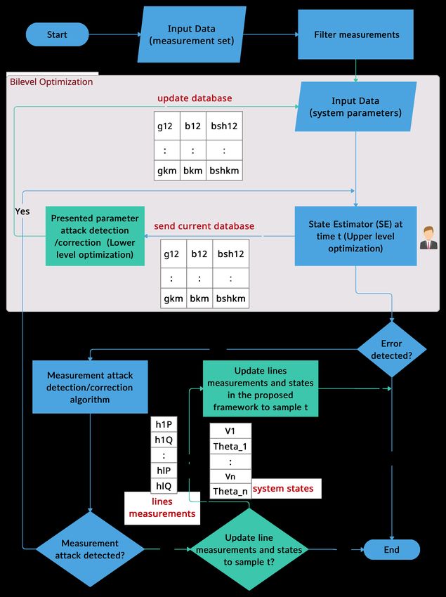
The flowchart of the presented framework is shown in Figure 1.
As illustrated in Figure 1, from the prospective of SE, the process starts by uploading
data of measurements and system model parameters. The SE routine is executed by system
operator every often to monitor the grid. The framework presented in Section 3.3 is initial-
ized with a true sample that is free from measurement and parameter errors. This sample is
labeled as t− . Then, for a sample t, SE routine is performed. On such, the bi-level model is
executed. If SE detects an error, then the presented inner (lower) level model in Section 3.3
is performed to check if the error source is due to measurement model parameters. To do
so, current status of the measurement model parameters are sent to the presented model
to be executed. After execution, if errors in line parameters are above certain threshold,
defined considering a level of confidence, then the corresponding line is updated to the
solution obtained by the model in Section 3.3 and SE is executed again. Otherwise, no
parameter error is detected [19]. If error is detected after updating measurement model
parameters, then the source of this error is due to errors in measurement. In such case, [30]
is run. After correcting errors from data at sample t, the base data in the presented model
can be updated if the sample t is trusted by system operator. Considering Figure 1, the
contribution of this work towards the WLS SE state-of-the-art process is highlighted with
the boxes colored in green.Appl. Sci. 2021, 11, 6540 8 of 15
Figure 1. Flowchart of the inclusion of the proposed framework.
4. Case Study
The presented bi-level model was validated using the IEEE 118-bus system. By
using the MATLAB package MATPOWER [31], 21,600 samples (i.e., one day’s worth) of
measurements were generated with Gaussian noise based on a common daily load profile
that contains temporal information of a power system’s changing state. The measurement
set includes real and reactive power flows, power injections, and all voltage magnitudes,
resulting in 712 measurements with Global Redundancy Level (GRL = m/N) of 3.029,
which relates the number of measurements (m) to the number of states (N) to be estimated.
Measurement’ standard deviations are considered as 1% of their absolute values. For
optimization, Gurobi solver [32] is used for solving the bi-level model. All simulations are
conducted on a personal Apple Mac computer: macOS High Sierra 32 GB RAM 1876 MHz
DDR3, 4 GHz Intel Core i7.
Towards validation, five independent 100 Monte Carlo simulations were conducted
for a selected sample. In each simulation, a line is selected randomly to have cyber-attacks,
modeled as FDI in model parameters, i.e, gkm , bkm , and bkmsh . The size of the cyber-attacks is
drawn from a uniform distribution between ±5% and ±40% of their actual values. The
optimization framework presented in Section 3.3 and Figure 1 is conducted after each
attack. Case study results are presented in Figure 2. Figure 2 shows that the absolute error
after correcting line parameters is less than an order of 3.
To further evaluate the accuracy and performance of the presented bi-level model,
around 20% of the samples (out of 21,600) are selected randomly to be compromised with
parameter cyber-attacks. Each of those samples, a random line is selected to have a FDI
parameter attack. The attack is in the same range as those performed for the aforementioned
simulations. The confusion matrix for the SE output using χ2 test as a detection method is
illustrated in Table 1. The χ2 threshold is calculated based on two parameters: number ofAppl. Sci. 2021, 11, 6540 9 of 15
measurements and confidence level. In this test, the number of measurements is 712 and
the confidence level is chosen to be 95% [19]. As seen, a substantial amount of samples
were not detected by χ2 test. Meanwhile, the presented bi-level model was executed
after each SE run. All anomaly samples were not only detected, but also corrected in a
single optimization run. Observed errors in correction were similar to the results shown
in Figure 2. The execution time of the proposed model was monitored for all anomaly
samples. On average, for 170 lines, the total execution time was 0.3964 s with a standard
deviation of 0.0533 s. It is worth mentioning that these reported statistics are without using
parallel computation. Hence, a lower execution time could be achieved with parallelism.
Figure 2. Absolute error in log scale.
Table 1. SE performance result for parameter attack detection χ2 test [19].
Prediction Outcome
Normal Anomaly
17336 0
Normal Normal
Actual
value
sample sample
3252 1012
Anomaly Anomaly
sample sample
Normal Anomaly
The CME N methodology presented in [30] for parameter attack processing, which
is the composed measurement error CME in its normalized form, is also explored in the
comparative test case scenarios. An anomaly sample is selected and the resulted CME N of
the measurements were listed in a descending order based on their absolute values for a
threshold value of 3. In this sample, the underlying true attack is on line connecting bus
94 and bus 95. The result is shown in Table 2. Based on the strategy presented in [30], the
attack is characterized as a parameter attack. However, not a specific line is determinedAppl. Sci. 2021, 11, 6540 10 of 15
as the one that is compromised. Instead, a region where the attack might be at could be
inferred. Hence, the superiority of the proposed framework is that it can identify and
correct the attack in a single process. In addition, it can be used as a pre-processing step
prior executing SE routine.
Table 2. Parameter Cyber-attacks Identification [30].
Measurement From Bus To Bus CME N
Real Power Flow 96 95 10.093
Reactive Power Flow 95 96 9.5299
Reactive Power Flow 94 95 7.9748
Reactive Power Flow 94 96 7.7034
Real Power Flow 94 95 6.3127
Real Power Flow 94 96 5.8595
Real Power Injection 95 95 4.0285
For stealthy attack, a line is selected and its parameters, i.e., g, b and bsh are attacked
gradually from 0 to 20% of their values. The performance index J as well as the CME in
its normalized form (CME N ) are recorded. The results are shown in Figures 3 and 4. In
Figure 3, the performance index J ( x ) (colored in blue) increased with the increase size of
the attack in the line’s parameters under attack. In this case, even though the performance
index J ( x ) increased, the χ2 test still did not detect the error. For identification, the CME N
is obtained for every attack and the absolute error is calculated and presented in Figure 4.
As shown, due to the increase size of the attack in a single line, the error is spread into
multiple estimation of measurements. After each attack scenario, the bi-level model is
performed. The error due to correction of parameters is calculated and shown in Figure 5.
Figure 3. Performance Index (J) single line case.Appl. Sci. 2021, 11, 6540 11 of 15
Figure 4. CME N absolute error single line case.
Figure 5. Absolute error of line parameter correction single line case.
The same scenario of the previous stealth attack is simulated for multiple lines in
this case. The results are shown in Figures 6 and 7. As seen from the figures, a similar
trend has occurred. However, the errors in measurement estimation are increased. TheAppl. Sci. 2021, 11, 6540 12 of 15
bi-level model is performed and lines are corrected. The observed error in correction for
the stealthy attacks is presented in Figure 8.
Figure 6. Performance Index (J) multiple lines case.
Figure 7. CME N absolute error multiple lines case.Appl. Sci. 2021, 11, 6540 13 of 15
Figure 8. Absolute error of line parameter correction multiple line case.
5. Conclusions
This paper presents a bi-level model for correcting parameter FDI cyber-attacks on the
SE process. The presented model combines the two processed that are usually performed
by SE for detection and correction into a single process for parameter attack processing. The
presented model can be used as a post-state estimation cyber-attack processing or prior to
validate the database of measurement model parameters and measurements. Meanwhile,
the framework can be used as an online tool due to the capability of performing parallel
computations. In addition, most the information needed in this framework is already
available among the data set used by SE. Comparative test results on the IEEE 118-bus
system show that the presented model is able to correct parameters with high accuracy,
while further processing measurement cyber-attacks. The existing state estimator software
can be adjusted to incorporate the presented framework without major modifications,
enabling the current work to be utilized by utilities. The model can be solved by solvers
that do not require sophisticated features.
Author Contributions: Conceptualization, N.A.; methodology, N.A.; software, N.A.; validation,
N.A.; formal analysis, N.A.; investigation, N.A.; resources, N.A.; data curation, N.A.; writing—
original draft preparation, N.A.; writing—review and editing, N.A. and A.B.; visualization, N.A.;
supervision, A.B.; project administration, A.B.; funding acquisition, A.B. All authors have read and
agreed to the published version of the manuscript.
Funding: This work was supported by NSF grant ECCS-1809739.
Institutional Review Board Statement: Not applicable.
Informed Consent Statement: Not applicable.
Data Availability Statement: Data are contained within the article.
Conflicts of Interest: The authors declare no conflict of interest.Appl. Sci. 2021, 11, 6540 14 of 15
References
1. Raiyn, J. A survey of cyber attack detection strategies. Int. J. Secur. Its Appl. 2014, 8, 247–256. [CrossRef]
2. Gupta, R.; Tanwar, S.; Tyagi, S.; Kumar, N. Machine learning models for secure data analytics: A taxonomy and threat model.
Comput. Commun. 2020, 153, 406–440. [CrossRef]
3. Sornsuwit, P.; Jaiyen, S. Intrusion detection model based on ensemble learning for U2R and R2L attacks. In Proceedings of
the 2015 7th International Conference on Information Technology and Electrical Engineering (ICITEE), Chiang Mai, Thailand,
29–30 October 2015; pp. 354–359.
4. Magalhaes, A.; Lewis, G. Modeling Malicious Network Packets with Generative Probabilistic Graphical Models. Available online:
http://cs229.stanford.edu/proj2016spr/report/021.pdf (accessed on 13 July 2021).
5. Jeya, P.G.; Ravichandran, M.; Ravichandran, C. Efficient classifier for R2L and U2R attacks. Int. J. Comput. Appl. 2012, 45, 28–32.
6. Liu, Y.; Ning, P.; Reiter, M.K. False data injection attacks against state estimation in electric power grids. ACM Trans. Inf. Syst.
Secur. 2011, 14, 1–33. [CrossRef]
7. Hug, G.; Giampapa, J.A. Vulnerability assessment of AC state estimation with respect to false data injection cyber-attacks.
IEEE Trans. Smart Grid 2012, 3, 1362–1370. [CrossRef]
8. Sridhar, S.; Manimaran, G. Data integrity attacks and their impacts on SCADA control system. In Proceedings of the IEEE PES
General Meeting, Minneapolis, MI, USA, 25–29 July 2010; pp. 1–6.
9. Bi, S.; Zhang, Y.J.A. Graph-based cyber security analysis of state estimation in smart power grid. IEEE Commun. Mag. 2017,
55, 176–183. [CrossRef]
10. Ozay, M.; Esnaola, I.; Vural, F.T.Y.; Kulkarni, S.R.; Poor, H.V. Sparse attack construction and state estimation in the smart grid:
Centralized and distributed models. IEEE J. Sel. Areas Commun. 2013, 31, 1306–1318. [CrossRef]
11. Kosut, O.; Jia, L.; Thomas, R.J.; Tong, L. Malicious data attacks on the smart grid. IEEE Trans. Smart Grid 2011, 2, 645–658.
[CrossRef]
12. Teixeira, A.; Sou, K.C.; Sandberg, H.; Johansson, K.H. Secure control systems: A quantitative risk management approach.
IEEE Control Syst. Mag. 2015, 35, 24–45.
13. Alexopoulos, T.A.; Korres, G.N.; Manousakis, N.M. Complementarity reformulations for false data injection attacks on PMU-only
state estimation. Electr. Power Syst. Res. 2020, 189, 106796. [CrossRef]
14. Hao, J.; Piechocki, R.J.; Kaleshi, D.; Chin, W.H.; Fan, Z. Sparse malicious false data injection attacks and defense mechanisms in
smart grids. IEEE Trans. Ind. Inform. 2015, 11, 1–12. [CrossRef]
15. Jin, M.; Lavaei, J.; Johansson, K.H. Power grid AC-based state estimation: Vulnerability analysis against cyber attacks. IEEE Trans.
Autom. Control 2018, 64, 1784–1799. [CrossRef]
16. He, Y.; Mendis, G.J.; Wei, J. Real-time detection of false data injection attacks in smart grid: A deep learning-based intelligent
mechanism. IEEE Trans. Smart Grid 2017, 8, 2505–2516. [CrossRef]
17. Ruben, C.; Dhulipala, S.; Nagaraj, K.; Zou, S.; Starke, A.; Bretas, A.; Zare, A.; McNair, J. Hybrid data-driven physics model-based
framework for enhanced cyber-physical smart grid security. IET Smart Grid 2020, 3, 445–453. [CrossRef]
18. Nagaraj, K.; Zou, S.; Ruben, C.; Dhulipala, S.; Starke, A.; Bretas, A.; Zare, A.; McNair, J. Ensemble CorrDet with adaptive statistics
for bad data detection. IET Smart Grid 2020, 3, 572–580. [CrossRef]
19. Bretas, A.S.; Bretas, N.G.; Carvalho, B.E. Further contributions to smart grids cyber-physical security as a malicious data attack:
Proof and properties of the parameter error spreading out to the measurements and a relaxed correction model. Int. J. Electr.
Power Energy Syst. 2019, 104, 43–51. [CrossRef]
20. Zou, T.; Bretas, A.S.; Ruben, C.; Dhulipala, S.C.; Bretas, N. Smart grids cyber-physical security: Parameter correction model
against unbalanced false data injection attacks. Electr. Power Syst. Res. 2020, 187, 106490. [CrossRef]
21. Bretas, N.G.; Bretas, A.S. A two steps procedure in state estimation gross error detection, identification, and correction. Int. J.
Electr. Power Energy Syst. 2015, 73, 484–490. [CrossRef]
22. Lin, Y.; Abur, A. Fast Correction of Network Parameter Errors. IEEE Trans. Power Syst. 2018, 33, 1095–1096. [CrossRef]
23. Abur, A.; Zhu, J. Identification of parameter errors. In Proceedings of the IEEE PES General Meeting, Minneapolis, MI, USA,
25–29 July 2010; pp. 1–4.
24. Carvalho, B.; Bretas, N.; Bretas, A. A local state vector augmentation technique for processing network parameters errors. In
Proceedings of the 2017 IEEE Power Energy Society General Meeting, Chicago, IL, USA, 16–20 July 2017; pp. 1–5.
25. Bretas, A.; Bretas, N.; Braunstein, S.; Rossoni, A.; Trevizan, R. Multiple gross errors detection, identification and correction in
three-phase distribution systems WLS state estimation: A per-phase measurement error approach. Electr. Power Syst. Res. 2017,
151, 174–185. [CrossRef]
26. Lin, Y.; Abur, A. Robust state estimation against measurement and network parameter errors. IEEE Trans. Power Syst. 2018,
33, 4751–4759. [CrossRef]
27. Arturo, B.; Newton, G.; Bretas, J.L.J.; Carvalho, B.E. Cyber-Physical Power Systems State Estimation; Elsevier: Amsterdam,
The Netherlands, 2021; Volume 1.
28. Bretas, N.G.; Bretas, A.S. The Extension of the Gauss Approach for the Solution of an Overdetermined Set of Algebraic Non
Linear Equations. IEEE Trans. Circuits Syst. II Express Briefs 2018, 65, 1269–1273. [CrossRef]
29. Sinha, A.; Malo, P.; Deb, K. A review on bilevel optimization: From classical to evolutionary approaches and applications.
IEEE Trans. Evol. Comput. 2017, 22, 276–295. [CrossRef]Appl. Sci. 2021, 11, 6540 15 of 15
30. Bretas, A.S.; Bretas, N.G.; Carvalho, B.; Baeyens, E.; Khargonekar, P.P. Smart grids cyber-physical security as a malicious data
attack: An innovation approach. Electr. Power Syst. Res. 2017, 149, 210–219. [CrossRef]
31. Zimmerman, R.D.; Murillo-Sanchez, C.E.; Thomas, R.J. MATPOWER: Steady-State Operations, Planning, and Analysis Tools for
Power Systems Research and Education. IEEE Trans. Power Syst. 2011, 26, 12–19. [CrossRef]
32. Gurobi Optimization, LLC. Gurobi Optimizer Reference Manual; Gurobi Optimization, LLC: Beaverton, OR, USA, 2021.You can also read