IJSOM - International Journal of Supply and Operations ...

International Journal of Supply and Operations Management

 IJSOM
 February 2021, Volume 8, Issue 1, pp. 1-17
 ISSN-Print: 2383-1359
 ISSN-Online: 2383-2525
 www.ijsom.com

 Robust Bi-Objective Location-Arc Routing Problem with Time Windows:
 A Case Study of an Iranian Bank
 Atefeh Kahfia, Reza Tavakkoli-Moghaddama,*, Seyed-Mohammad Seyed-Hossenib
 a School of Industrial Engineering, College of Engineering, University of Tehran, Tehran, Iran
 b Schoolof Industrial Engineering, Iran University of Science and Technology, Tehran, Iran

Abstract
In Location-Arc Routing Problems (LARP), unlike the well-known locating-routing problems, demand is on the arc and using
deadheading arcs is permitted. Few studies have focused on an arc-routing problem. In this research, a complex bi-objective
linear mathematical model for the LARP with time windows under uncertainty is presented. Time windows in the arc-routing
problem modeling have complexity since the required arc with time windows becomes a deadheading arc without time windows
after service. Furthermore, modeling of the vehicle servicing to multiple required arc with the minimum deadheading arc in
route is a feature of this work. The proposed LARP is used for modeling of transforming cash in the bank case study. In this
case study, demand has uncertainty with unknown probability distributions and we used Bertsimas and Sim approach for it. The
case study problem is a node-basing problem with the closest node and time windows for servicing branches. For this purpose,
the Multi-Objective Dragonfly Algorithm (MODA) and Non-dominated Sorting Genetic Algorithm (NSGA-II) are used for
locating the cash supply centers of a bank in Tehran. Furthermore, comparing results of robust and deterministic LARP models
show that the mean and standard deviation of objective function values in the robust model has better performance in realization.

Keywords: Location-arc routing problem; Time windows; Multiple periods; Robust optimization; Demand Uncertainty.

1. Introduction
The aim of a routing problem is to select the optimal routes for vehicles to service the customers considering limitations,
equipment, and objectives. In this problem, customers are located on the node or arc/edge of a graph. The Vehicle Routing
Problem (VRP) is the node routing problem and the Rural Postman Problem (RPP) is the arc routing problem. Some
researchers have focused on arc routing problems recently.
The Capacitated Arc Routing Problem (CARP) is an expansion of the RPP with multi-vehicle and capacity conditions
(Golden and Wong, 1981). This problem is defined on an undirected connected graph = ( , ) that each edge (i.e.,
customer) has a demand ≥ 0. For serving required edges, undemanded (deadheading) edges with minimum numbers
must be used. After servicing the required edge, it becomes a deadheading edge and can services other required edges.
A Location-Arc Routing Problem (LARP) is a combination of the CARP and the Location-Allocation Problem (LAP) (Ghiani et
al., 2001). The LARP is defined as a graph that can be directed, undirected or both. The crucial difference between the CARP and
the LARP is that along with routing, the best depot location must be determined. Therefore, this issue is added as a binary decision
variable to the mathematical model and makes it even more complicated. The LARP can be used for arc-routing problems (e.g.,
snow plowing or node-routing problems) with nearby nodes (e.g., the distribution network of supermarkets) (Albareda-Sambola,
2015). Limited studies have been focused on the second application of the LARP (Tavakkoli-Moghaddam et al., 2018).

* Corresponding author email address: tavakoli@ut.ac.ir
DOI: 10.22034/IJSOM.2021.1.1

 1

Kahfi, Tavakkoli-Moghaddam and Seyed-Hosseni

1.1. Contribution
The main purpose of this paper is to solve transforming the problem of cash in the branches network in a bank. This
problem is to select an optimal number and the location of the cash supply center as well as the optimal routing for cash
delivery to branches. In the case study, four cash supply centers are carried out delivery and collection of cash to 517
banking units (i.e., 250 branches, 202 counters, and 65 fuel stations) in Tehran. Three cash supply centers have been
closed and bank has a challenge for delivery and collection of cash on time. This is a node routing problem with nodes
close and can be considered as an arc routing problem for solving it. Therefore, in the case study, branches with a distance
of less than 1 km and similar availability can be considered as a required arc with the sum of branches demand. In the
case study, delivering and collecting cash on time are necessary, and the definition of time windows constraint is
important. Considering the time windows in the arc-routing problem has a different structure than the node-routing
problem, since a required arc with time windows after servicing can be used as a deadheading arc without time windows
as a path. The waiting time of the vehicle in servicing time is minimized considering the low probability of rubbery,
indirectly. The number of cash supply centers, vehicles, and equipment depends on the demand for cash collection or
delivery. This demand is uncertain due to uncertainty in the factors affecting the liquidity of the society (Pavlis et al.
2018). Therefore, a robust approach is used for uncertain demand. This paper presents a bi-objective and multi-period
LARP model with time windows under uncertainty to minimize the cost and waiting time. The deterministic and robust
LARP model are solved by the Multi-Objective Dragonfly Algorithm (MODA) and Non-dominated Sorting Genetic
Algorithm (NSGA-II) under nominal data and realization.

1.2. Organization
The rest of this paper is structured as follows. Section 2 is associated with the literature review, including the LARP, time
windows in an arc routing problem, and robust approach. In Section 3, a robust mathematical model for the LARP is
presented. The case study is described in Section 4. In Section 5, the MODA and solution representation are explained.
To evaluate the performance of the proposed deterministic and robust models are solved by the MODA and NSGA-II for
the bank case study in Section 6. Finally, this paper is concluded in Section 7.

2. Literature review
The number of LARP researches are increased, recently. However, LARP has a higher complexity versus to Location-
Routing Problem (LRP), and many features such as time window, uncertainty needs to be surveyed in this problem.

2.1. Review of location-arc routing problems
The LARP was proposed by Levy and Bodin (1989) to solve the routing problem at the post office in the USA. They used
a Location-Allocation-Routing method to solve this model. Ghiani and Laporte (2001) presented a linear multi-depot
model for the LARP. They converted it to RPP model and solved it by a branch-and-cut. Liu et al. (2014) presented a
survey of recent researches on LARP. The specifications of the LARP are addressed in Table 1.
Doulabi and Seifi (2013) presented two MILP models for single and multi-depot problems with the flow variables and
solved them by simulated annealing. Lopes et al. (2014) proposed a LARP mathematical model and solved it by several
heuristics. They tested different constructive heuristics combining variable neighborhood search, greedy randomized
adaptive search procedure, and tabu search. Their model implies each customer has required an individual vehicle that is
not practical. Laporte et al. (2015) developed LARP models presented by Doulabi and Seifi (2013) and Lopes et al.
(2014). They solved their model with the exact method. Essink and Wagelmans (2015) used Lopes et al. (2014) model
and solved it by metaheuristic TS-GRASP. Riquelme-Rodríguez et al. (2016) proposed a non-linear model for a periodic
LARP and used a heuristic method for solving their model. Huber (2016) presented a bi- objectives model without
formulating constraints. He used heuristic method for solving benchmark instances. Amini et al. (2017) addressed an
uncertain LARP and employed two scenario-based approaches. They evaluated the performance of models with the results
of the numerical example.
Tavakkoli-Moghaddam et al. (2018) presented a multi-product LARP by developing two mathematical models under two
assumptions. All types of products of a required arc must be supplied by a tour and each type of a required arc product
must be supplied by a tour. Fernández et al. (2019) modeled several LARPs on an undirected graph and solved them with
branch and cut. Amini et al. (2019) developed the LARP when there are transportation decisions from suppliers to
established depots. They used augmented ε-constraint, NSGA-II, and Multi-Objective Late Acceptance Hill-Climbing

 Int J Supply Oper Manage (IJSOM), Vol.8, No.1 2

Robust Bi-Objective Location-Arc Routing Problem with Time Windows: a Case Study of an Iranian Bank

algorithm for solving this problem. Mirzaei-Khafri et al. (2019) considered a CLARP with deadlines and a fleet of
capacitated heterogeneous vehicles. They showed that the result of the sensitivity analysis of their proposed model can
meet arc routing timing requirements more precisely compared to the CARP.

2.2. Time windows in an arc routing problem
In this paper, the time window is important for servicing branches of the bank case study. The CARP researches address
this concept. Vansteenwegen et al. (2010) used a meta-heuristic method to solve the ARP problem with soft time windows
for a case study of the mobile mapping van problem. They did not present any mathematical programming model. Macedo
et al. (2011) are not modeled time window and solved it with metaheuristic methods. Lystlund et al. (2012) presented two
linear models for the CARP problem with hard and soft time windows and solved it with the heuristic. Black et al. (2013)
define a CARP model with prize-collecting. The proposed model was non-linear that was not possible to linearize.
Therefore, a heuristic method has been used for solving the model. Çetinkaya et al. (2013) claim that it is not possible to
model time windows in arc routing problems and should be transformed into a node routing problem. They did not present
a model for the ARP with time windows and prize-collecting and used a meta-heuristic to solve it. Çetinkaya et al. (2018)
proposed a model for the LRP by defining time windows for arcs with military applications. While in the proposed model,
the time window is defined for arcs, the customers are located on the nodes and the model is node-based.

 Table 1. Comparison of LARP features
 Depot Customer Vehicle Material Determine the number Model Features
 Solving Method
 Splitting allowed

 Multi-objective
 Time Windows
 Heterogeneous

 Heterogeneous
 Time available
 Multi Produce

 Game theory
 Multi-period
 Multi depot

 Uncertain
 Inventory

 Capacity
 Capacity

 Capacity

 Metaheuristic
 Linear
 Risk
 Reference

 heuristic
 Exact
 (Doulabi & Seifi, 2013) × × × × ×
 (Lopes et al., 2014) × ×
 (Essink & Wagelmans, 2015) × × × ×
 (Riquelme-Rodríguez et al., 2016) × × ×
 (Huber, 2016) × × × ×
 (Amini et al., 2017) × × × ×
 (Tavakkoli-Moghaddam et al., 2018) × × × × ×
 (Javanmardi & Hafezalkotob, 2018) × × × × ×
 (Fernández et al., 2019) × × ×
 (Amini et al., 2019) × × × × ×
 (Mirzaei-Khafri et al., 2019) × × × ×
 (Mirzaei-Khafri et al., 2020) × × × × ×
 This paper × × × × × × × × × × × × × ×

2.3. Uncertainty in arc routing problem
The main approaches to deal with data uncertainty in optimization are stochastic, fuzzy and robust programming. These
approaches have different applications (Teimoori et al., 2014; Fazli-Khalafa, Hamidieh, 2017; Hamidieha et al., 2018).
Stochastic programming i.e. Scenario-based stochastic programming can be applied for probabilistic randomness data.
Fuzzy programming is like stochastic programming and the difference is in the way uncertainty is modeled. Robust
optimization approaches can be used for data with unknown probability distributions. A robust approach is a method for
solving problems of linear optimization under uncertain conditions. To ensure that the solution remains near-optimal and
feasible when the data changes, this approach has accepted a sub-optimal solution for nominal data values. Optimal
solutions that are less sensitive to uncertainty is called a robust solution (Bertsimas & Sim, 2004). This method is an
alternative for stochastic programming and sensitivity analysis that is used in discrete problems. Different models have
been developed to formulate linear optimization problems with robust methods. Three primary models in a robust
approach based on interval uncertainty are Soyster (1973), Ben-Tal and Nimrovsky (1998), and Bertsimas and Sim (2004).
The Soyster approach is the most conservative method among others, such that the objective value is much worse than
the objective value of nominal linear optimization problem. Ben-Tal and Nimrovsky approach is a quadratic conical

 Int J Supply Oper Manage (IJSOM), Vol.8, No.1 3

Kahfi, Tavakkoli-Moghaddam and Seyed-Hosseni

model with + 2 variable and + 2 constraint. Since this model is non-linear, it is not efficient solution for discrete
optimization models. The Bertsimas and Sim (2004) approach change the linear programming (a) to a robust model (b)
as follows:

 Min Min + 0 Γ0 + ∑ 0 
 ∈ 0

 s. t. s. t.

 ∑ ̃ ≤ ∀ (a) ∑ + Γ + ∑ ≤ ∀ (b)
 ∈ 
 
 ≤ ≤ + ≥ ̂ ∀ ≠ 0, 

 0 + 0 ≥ ∀ 

 ≤ ≤ ∀ 

 , , ≥ 0 ∀ , 

where coefficients ̃ are uncertainty and random variable in [ − ̂ , + ̂ ], and ̂ are the nominal values
and the variation magnitude of the uncertain parameter, respectively. denote the set of uncertain coefficients of row i.
For the i-th constraint, a control parameter , is called the price of robustness. Parameters [0, | |] and | | are the
cardinality of the set .
Babaee Tirkolaee et al. (2018) presented a robust periodic CARP for urban waste collection considering drivers and
crew’s working time. Babaee Tirkolaee et al. (2019) proposed a robust bi-objective multi-period CARP for urban waste
collection using a Multi-Objective Invasive Weed Optimization (MOIWO). Babaee Tirkolaee et al. (2020) consider the
multi-trip CARP under fuzzy demands for urban solid waste management. Mirzaei-Khafri et al. (2020) consider a
location-arc routing problem (LARP) on an undirected network. The proposed robust model was less sensitive to demand
variations and was validated through Monte-Carlo simulation and Relative Extra Cost (REC) measures with promising
results. The results of sensitivity analysis showed that by increasing the degrees of conservatism, planners might employ
more vehicles. Also, more depots might be opened to service all required roads.
The literature review in this section shows that the models for LARPs do not address time windows. The review of arc
routing researches with time windows shows that a few researches focus on presenting a mathematical model, and all
models except Lystlund et al. (2012) are non-linear. Besides, the models for LARPs are not used for the financial case
study. The scenario-based stochastic programming and fuzzy approach to deal with data uncertainty in the models for
LARPs are used and robust programming is not used so far.

3. Mathematical model
The LARP is defined as a graph = ( , ∪ ), which = { , … . , } is a set of vertex,
 = {[ , ]: , ∈ , ≠ } is a set of edges, and = {( , ): , ∈ , ≠ } is a set of arcs, which can be directed,
undirected, or a combination of both. Here, the LARP problem is a directional graph and the connection of two vertexes
is called an arc. The vertex set contains a non-empty subset of potential
depot locations ( ⊆ ). Every arc ( , ) ∈ has a non-negative traversal cost and a non-negative demand for service.
The arcs with positive demand form the subset A of the arcs required to be serviced, only once, by a vehicle K with
capacity Q in a determined time window. Vehicles start and end their route in the same depot, and each new vehicle. The
deadheading arc is movement from the end i of one required arc to the start j of another required arc without servicing the
traversed arcs.
The assumptions, sets, parameters, uncertain parameters, decision variables for robust bi-objective LARP model are
presented in the following subsections.

 Int J Supply Oper Manage (IJSOM), Vol.8, No.1 4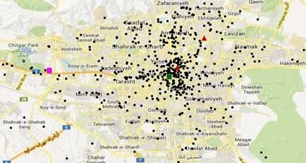

Robust Bi-Objective Location-Arc Routing Problem with Time Windows: a Case Study of an Iranian Bank

3.1. Assumptions
The main assumptions are as follows:
  Every required arc is traversed by one vehicle
  The vehicle is returned to the depot that was started
  The total demand for the arcs selected on tour is less than the vehicle capacity
  The number of deadheading arc selected in every tour is minimized
  Each required arc is serviced once that can be used as a deadheading arc without a time windows
  Waiting time is allowed for each required arc at the start of service
  The distribution of products is delivery and collection
  The number of deadheaded traverses in each arc is not limited

3.2. Sets, parameters, and decision variables
Sets, parameters, and decision variables used in mathematical models are as follow:

Sets
I Set of all vertices (I = {1, ..., i}, which includes customers and depots)
J Set of depots ( = {1, … , ′ } that ′ is the maximum number of depots)
K Set of vehicle = {1, … , }
P Set of period = {1, … , }
S Set of steps that every vehicle travels = {1, … , }
A Set of required arcs that has to be visited
 Set of vertices that are extremities of the arcs in set A
 ̂ Union of the set J and ( ̂ = ∪ )
 ̂ Set of arcs forming a complete graph with ̂
 + ( )( − ( )) Set of arcs leaving (entering) on the set of vertices J. When S contains a single vertex v, + ( ) is a
 simplification for + ({ })

Parameters
 ′ Costs of creating a depot ′ in period p
 Costs of traversing arc ( , ) in period p, if arc ( , ) ∈ cost of servicing is equal to ̂ and if the arc is
 deadheading (i.e. arc ( , ) ∉ ) is equal ́ 
 ′ The capacity of depot j in period p
 Travel time on arc ( , ) ∈ in period p, if arc ( , ) ∈ time of traveling is equal to ̂ and if the arc is
 deadheading (i.e., arc ( , ) ∉ ) is equal arcs ́ 
 The maximum time allowable for vehicle k in period p
 Fixed costs of using vehicle k
 The number of customers in period p
 The capacity of vehicle k in period p
M A very large number

 Int J Supply Oper Manage (IJSOM), Vol.8, No.1 5

Kahfi, Tavakkoli-Moghaddam and Seyed-Hosseni

Uncertain Parameter
 ̃ Demand for service of arc ( , ) ∈ 
Decision variables
 1 if arc ( , ) ∈ ̂ is traveled by vehicle k in period p at step s; and 0, otherwise
 1 if arc ( , ) ∈ is serviced by vehicle k in period p at step s; and 0, otherwise
 ′ 1 if arc ( , ) ∈ is allocated to depot j' in period p
 The time that service of the arc ( , ) ∈ ̂ starts
 The time that vehicle k arrives in node i at step s
 The time that vehicle k starts traversing arc ( , ) ∈ ̂ at step s
 Slack variable for eliminating sub-tours

3.3. Robust bi-objective LARP model
The first proposed LARP model is bi-objective, multi-period, and mixed-integer non-linear programming with uncertain
demand. Finally, the proposed model is converted into a linear and robust model.

3.3.1. Objective functions
The objective function (1) minimizes the sum of the costs of depots creation, serviced arcs, and selected vehicles,
respectively. The second objective (2) minimizes the waiting time of the vehicle.

 Min 1 = ∑ ∑ ′ ′ + ∑ ∑ ∑ ∑ + ∑ ∑ ∑ ∑ (1)
 ′ ( , ) ̂ ( , )∈ + ( ) 

 Min 2 = ∑ ∑ ∑ ∑( − ) (2)
 ( , ) \{1} 

3.3.2. Basic Constraints
Standard LARP includes basic Constraints (3-11). Constraint (3) ensures that each required arc is serviced once by
precisely one vehicle. Constraint (4) guarantees that the flow is preserved i.e., the number of arrivals at any node is equal
to the number of leaving. Constraint (5) implies that an arc is serviced by a particular vehicle only if it is traversed by the
same vehicle. Constraint (6) is a sub-tour elimination constraint. A tour is started from a depot and is ended at the same
depot. The constraint of allocated of the required arcs to a depot is defined by ∑ ′ ≤ M ′ . This
constraint is non-linear. Therefore, ′ × , replaced by ℎ ′ . Besides, this constraint is replaced with Constraints
(7-9). The constraints make sure all required arcs that are in the same route are devoted to depot j that route is started
from it and ended. This constraint forced the vehicle to service to multiple required arc. These constraints are necessary
to establish Constraint (10) that ensures the capacity of the depots is not violated. Constraint (11) ensures that the vehicle
capacity is not exceeded.

 ∑ = 1 ∀ ( , ) , , (3)
 
 ∑ − ∑ = 0 ∀ , , , (4)
 ( , ) + ( ) ( , ) − ( )

 Int J Supply Oper Manage (IJSOM), Vol.8, No.1 6

Robust Bi-Objective Location-Arc Routing Problem with Time Windows: a Case Study of an Iranian Bank

 ≥ ∀ ( , ) , , , (5)

 − + ≤ − 1 ∀ ( , ) , ≠ , , , (6)

 ℎ ′ ≤ ′ ∀ ′ , , ( , ) , , (7)

 ′ + ≤ 1 + ℎ ′ ∀ ′ , , ( , ) , , (8)

 ′ + ≥ 2 ∗ ℎ ′ ∀ ′ , , ( , ) , , (9)

 ∑ ̃ ′ ≤ ′ ∀ ′ , , , (10)
 ( , ) 

 ∑ ̃ ≤ ∀ , , (11)
 ( , ) 

3.3.3. Time windows constraint
Time window constraints are summarized in Constraints (12) – (19). The time windows in the arc routing problem have
a different structure compared to the node routing problem. After servicing a required arc, we can use it as a deadheading
arc without time windows. Constraint (12) denotes that the start time of the journey on arc ( , ) ̂ cannot be before the
arrival time in node i at step s. Index s is steps that every vehicle travels. This index is necessary for Constraints (12) –
(19), since arrival time in node j is calculated based on arrival time in node i in previous step of vehicle. In standard
LARP, this index is not necessary.
Constraints (13) – (14) implies that if vehicle k services to the required arc ( , )ϵ , the arrival time in node j will equal
to sum of the start time and service time. Constraints (15) and (16) demonstrates that if vehicle k traverses the deadheading
arc ( , )ϵ ̂, the arrival time in node j will equal the sum of the start time and travel time. Constraints (13) – (16) are
functional constraints if the vehicle selects the arc for service or travel. Constraint (17) ensures that the service time
variable is equal to start time of servicing the vehicle. Constraint (18) ensures that required arc cannot be deadheading
arc earlier than finishing the service time. Constraints (12) – (18) are functional constraints if the required arc ( , )ϵ is
selected in optimum routes. Constraint (19) ensures that the vehicles, at the first step, will start in the depot at time zero.
Constraint (20) ensures that the vehicle usage time in each tour does not exceed the maximum available time.

 − ≤ (1 − ) ∀ ( , ) ̂, , , (12)

 + ́ − +1 ≤ (1 − ) ∀ ( , ) , , , (13)

 +1 − ( + ́ ) ≤ (1 − ) ∀ ( , ) , , , (14)

 + − +1 ≤ (1 − ( − )) ∀ ( , ) ̂, , , (15)

 +1 − ( + ) ≤ (1 − ( − )) ∀ ( , ) ̂, , , 
 (16)

 − ≤ (1 − ) ∀ ( , ) , , , 
 (17)

 + ́ − ≤ (1 − ( − )) ∀ ( , ) ̂, , , 
 (18)

 Int J Supply Oper Manage (IJSOM), Vol.8, No.1 7

Kahfi, Tavakkoli-Moghaddam and Seyed-Hosseni

 0 1 = 0 ∀ , (19)

 ∑ ≤ ∀ , (20)
 ( , ) 

3.3.4. Decision variables
Constraints (21) make sure that the decision variables are binary and non-negative.

 , , ′ , , ℎ ′ ∈ {0,1}, , , ≥ 0 (21)

If demand in Constraints (10) and (11) is considered determined, objectives function of (1) and (2) and Constraints (3) to
(21) are made the deterministic LARP model. In the bank case study, demand is uncertain with unspecified distribution
function. In the next subsection, we present a robust model for the LARP by using the approach proposed by Bertsimas
and Sim (2004).

3.3.5. Robust LARP model

In the proposed model for the LARP, ̃ ∈ [ − ̂ , + ̂ ] in Constraints (10) and (11) has uncertainty.
 1 1 1
Accordingly, based on Section 2.3, by introducing variables , and , Constraint (10) is replaced by the following
constraints:

 1
 + 1
 +∑ 1
 ≤ ∀ , (22)
 ( , ) 

 1
 1
 + ≥ ̂ ∀ ( , ) , , (23)

 1 1
 , ≥0 (24)

 2 2 2
Similarly, by introducing variables and and , Constraint (11) will be replaced with the these constraints:

 2
 ′ + 2
 +∑ 2
 ≤ ′ ∀ ′ , , (25)
 ( , ) 

 2
 2
 + ≥ ̂ ′ ∀ ( , ) , ′ , , (26)

 2 2
 , ≥0 (27)

Therefore, the proposed bi-objective robust model for the LARP is mixed-integer linear programming with objective
functions (1) and (2) and Constraints (3) – (9) and (12) – (27). This robust proposed model is used for solving the location
and routing problem of the bank as case study with uncertain demand for cash collection and delivery.

4. Bank case study
Processing the cash supply should be on time in the bank branches network. In this paper, the bank case study has two
challenges in the cash supply. Challenge 1: according to the instructions of the Central Bank of Iran, cash collection and
delivery should be done by the cash supply center of the bank or the National Bank by fee-paying. The cost-benefit of
these solutions should be calculated with the number and location of the required cash supply center. Kahfi et al. (2018)
solved this challenge with an LARP model. Challenge 2: the cash supply center of the bank in Tehran has several
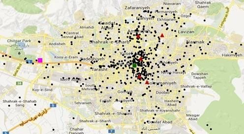
problems. In this case study, four cash supply centers (i.e., red, green, purple, and pink rectangles in Figure 1a) collect
and deliver the cash for 517 banking units (250 branches, 202 counters, and 65 fuel stations) in Tehran. Also, a special

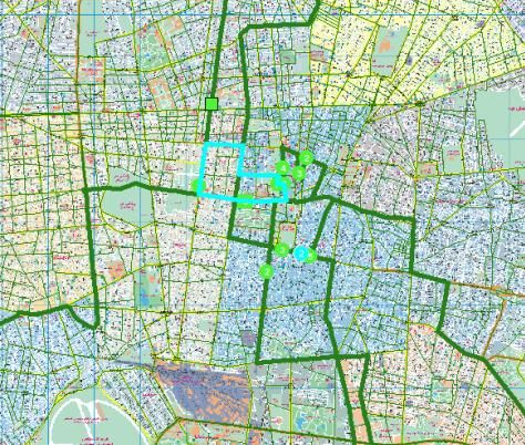
 Int J Supply Oper Manage (IJSOM), Vol.8, No.1 8

Robust Bi-Objective Location-Arc Routing Problem with Time Windows: a Case Study of an Iranian Bank

cash supply center (i.e.blue rectangles in Figure 1a) is communicated with the Central Bank of Iran and other cash supply.
The problems of the cash supply of the Tehran center are as follows:

  Two cash supply centers were included in the urban development planning (blue and purple in Figure 1a) the bank
 is forced to move them to another cash supply center (i.e., green rectangle in Figure 1a).

  One of the cash supply centers (red rectangle in Figure 1a) had security problems. Therefore, it moved to a
 temporary cash supply center (orange rectangle in Figure 1a).

 a) Current cash supply centers location

 b) Potential cash supply centers location
 Branches Current cash supply centers Potential cash supply centers

 Figure 1. Current and potential cash supply centers location

Therefore, there are three cash supply centers (i.e., green, orange, and pink rectangles in Figure 1a) that service all
branches in Tehran. These problems increase servicing time and transportation costs and decrease the security of cash
supply centers and cash transfers. Determining the optimum number of the cash supply center and its location in Tehran
was the main problem in this case study. Also, two cash supply centers are fixed. The potential locations are shown in
Figure (1b). This problem is a node-basing problem with the closest node that could be converted arc-routing problem
with smaller dimensions. For this purpose, branches with 2 km distance are replaced by the required arc. Therefore, 517
nodes in this case study problem are converted to 214 nodes that decrease problem dimensions.
In the case study, we use Tehran map with the required information, such as the branches location, the type of streets, the
type of traffic allowed, the width of the street and the length of the street. For this purpose, the GIS Bank team used
ArcMap 10 software. Figure 2 shows a small part of the map after identifying the permitted routes (bold green lines), the
selected routes (blue lines) and the branches (green circular).

 Int J Supply Oper Manage (IJSOM), Vol.8, No.1 9

Kahfi, Tavakkoli-Moghaddam and Seyed-Hosseni

 Figure 2. Part of the Tehran map with bank information

5. Solution approach
The proposed model for the LARP is NP-hard and bi-objective. Therefore, we use the MODA (Mirjalili, 2016) and
NSGA-II (Deb et al. 2002). To solve this model, first, we present a solution representation of the problem as a necessary
step in designing the algorithm. Then, we describe the MODA, a generation of the initial solution and a verified algorithm.

5.1. Solution representation
The solution representation in routing problems is based on a sequence of nodes number. Different solution representation
is introduced in the research paper (Armas et al., 2018). In Lacomme et al. (2004), the solution representation is as a
vector. The initial value of this vector is generated randomly that the vector is divided into several parts, and each part is
assigned to a vehicle. The infeasible vector will be removed. In Kirlik and Sipahioglu (2012), the solution representation
is defined as a matrix with a variable number of rows and columns, in which the number of rows is the number of the
vehicle. In this representation type, selecting the vehicles are always in order. In this research, a solution representation
is as a matrix with unknown dimensions (Figure 3a). The number of rows and columns is variable. The numbers of rows
and columns are dependent on routes and nodes that are serviced by the vehicle, respectively.
For example, in a problem with three depots and four vehicles, if the set of required arcs is {1-4, 4-5, 5-7, 5-8, 7-8, 8-6,
2-6, 2-4, 8-10, 2-10, 9-10, 3-7}, the solution representation is shown in Figure 3b. The first row shows that vehicle 2 is
assigned to depot 1 and services to the required arcs {1-4, 4-5, 5-8, 8-7, 7-5}. In route 2, the required arc of {8-5} is as a
deadheading arc that is serviced in route 1. This solution is presented in Figure 3c.

5.2. Multi-Objective Dragonfly Algorithm
The Dragonfly Algorithm (DA) is introduced by Mirjalili (2016). Dragonflies have special swarming behaviors. The aims
of dragonflies swarm are hunting (i.e., static swarm) and migration (i.e., dynamic swarm). Dragonflies in a static swarm
create small group that has abrupt changes and local movement in the flying path. The huge number of dragonflies in
dynamic swarms create swarms to migrate over long rout in one way. The DA is originated from static and dynamic
dragonflies swarming behavior. These two behavior are identical to the two main stages of optimization: exploration and
exploitation in meta-heuristic algorithms. Dragonflies make sub-swarms and fly in disparate locations in a static swarm
that is the aim of the exploration stage. In a dynamic swarm, dragonflies fly in larger swarms along one path that is the
main objective in exploitation. The multi-objective DA (MODA) is used to solve the presented multi-objective model.
The MODA is described in Figure 4.

 Int J Supply Oper Manage (IJSOM), Vol.8, No.1 10

Robust Bi-Objective Location-Arc Routing Problem with Time Windows: a Case Study of an Iranian Bank

 Nodes
 Vehicles Depots Vehicles Depots Nodes number
 number
 number number number number
 1 2 … 1 2 3 4 5 6 7
 Route 1 Route 1 2 1 4 5 8 7 5 1 -
 Route 2 Route 2 4 2 6 8 5 4 2 - -
 … Route 3 3 2 10 9 3 7 8 10 2
 a) Solution representation b) Sample solution representation

 4

 Required arc
 1 Serviced Traversed
 required arc deadheading arc
 5 2
 6 Open depot red – route 1
 blue – route 2
 Close depot orange – route 3
 8
 7 10

 9
 3
 c) A sample feasible solution
 Figure 3. Solution representation with a sample for the proposed LARP

 Initialize the dragonflies population Xi (i = 1, 2, ..., n) and step vectors ΔXi (i = 1, 2, ..., n)
 Define the maximum number of hyperspheres (segments) and the archive size
 While the end condition is not satisfied
 Calculate the objective values of all dragonflies
 Find the non-dominated solutions
 Update the archive for the obtained non-dominated solutions
 If the archive is full
 Run the archive maintenance mechanism to omit one of the current archive members
 Add the new solution to the archive
 End if
 If any of the new added solutions to the archive is located outside the hyperspheres
 Update and re-position all of the hyperspheres to cover the new solution(s)
 End if
 Select a food source from archive
 Update w, s, a, c, f, and e
 ∑ ∑ 
 Calculate S, A, C, F, and E using: = − ∑ 
 =1 − , =
 =1
 , = =1 − , = + − , = − + 
 
 Update neighboring radius
 Select an enemy from archive
 Update position vectors using
 If a dragonfly has at least one neighboring dragonfly
 Update the velocity vector using ∆ +1 = ( + + + + ) + ∆ and position vector using +1 = +
 ∆ 
 Else
 1⁄ 
 
 1 × Γ(1+β)×sin( )
 2
 Update position vector using +1 = + ́ ( ) × , ́ ( ) = 0.01 × 1 , =( 1| −1 ) , Γ(x) = ( − 1)!
 ( 2 )
 | 2 | Γ( )×β×2
 2
 End if
 Check and correct the new positions based on the boundaries of variables
 End while
 Figure 4. Pseudo-codes of the MODA

Where , , , + , − and are the position of the current dragonfly, the position of the j-th dragonfly in the
neighborhood, speed of the j-th dragonfly in the neighborhood, position of the food source, position of the enemy, and
the number of neighborhood dragonflies, respectively. Also, s, a, c, f, e are the coefficient of separation, alignment,

 Int J Supply Oper Manage (IJSOM), Vol.8, No.1 11

Kahfi, Tavakkoli-Moghaddam and Seyed-Hosseni

cohesion, attraction, the distraction of enemy, respectively. is the weight of inertia and is the counter of the algorithm.
Also, is the dimensions of the position vector, 1 and 2 are two random numbers in the interval [1-0] and are assumed
to be a constant value equal to 1.5. The position of dragonflies is updated using five factors as follows:
  Separation: Avoid colliding with other neighbors ( )
  Alignment: Adjust the speed with neighbors ( )
  Cohesion: Tendency to the center of gravity of neighbors ( )
  Attraction: Absorption to food sources ( )
  Distraction: Outward to enemy ( )

5.3. Initial solution Generation
To generate the initial solution, the following steps are performed:
1. Choose a random vehicle between the vehicles that have the volume and time capacity.
2. Choose a random depot between the depots that have the volume capacity.
3. Choose a random required arc with the following conditions:
 3.1. Start point is selected depot in Step 2.
 3.2. If the demand is less than the capacity of the depot, go to Step 3.3, otherwise, go back to Step 2. the number of this
 depot is added to the blacklist.
 3.3. If demand is smaller than the capacity of the vehicle and arc travel time is in time windows interval, the selected
 arc is removed from the required arc list and added to the deadheading arc list. Then, depot and vehicle capacity and
 vehicle time capacity are updated. Otherwise, go back to Step 1 and the vehicle number is added to the blacklist.
4. Choose a random required arc with the following conditions:
 4.1. If the ending node of selected arc is the starting node of another required arc goes to Step 4.2; otherwise, go to Step 6.
 4.2. If arc demand is less than the depot and vehicle capacity and arc travel time is in time windows interval, the selected
 arc is removed from required arc list and is added to deadheading arc list. The depot and vehicle capacity as well
 as vehicle time capacity are updated. Otherwise, return to Step 1 and add the vehicle number to the blacklist.
5. Choose a random deadheading arc with the following conditions and return to Step 4:
 5.1. Starting node arc is the ending node of selected arc in Step 4.
 5.2. Arc has smallest traveling time.
6. If all required arcs are serviced, go to the correction algorithm, otherwise, if the vehicle and depots are not on blacklist,
 go to step 4; otherwise, go back to Step 1 and the vehicle and depots add to the blacklist.

5.4. Correction algorithm
For an infeasible solution, the following corrective steps are required:
 1. If the end of vehicle route is not the depot, remove it from the solutions.
 2. If the route is not serviced by required arc, this route is deleted.
 3. If there are consecutive deadheading arcs on the route and there is a shorter route between the starting and ending
 nodes of these arcs, consecutive deadheading is replaced by this arc.

6. Experimental results
The LARP is an NP-hard problem with a large number of binary variables (Khajepour et al. 2020). In this paper, we use
the MODA to solve the proposed LARP for the case study problem. Also, the NSGA-II is used for the validation of the
MODA. This model is tested on a PC with Intel Pentium 4, core i5, 2.4 GHz processor with 4 GB memory. Also, The
Taguchi method is used for parameter tuning for the MODA and the NSGA-II (Table 2).

 Table 2. Parameter tuning with the Taguchi method

 Int J Supply Oper Manage (IJSOM), Vol.8, No.1 12

Robust Bi-Objective Location-Arc Routing Problem with Time Windows: a Case Study of an Iranian Bank

 Population size Separation Alignment Cohesion Attraction Distraction
 MODA
 400 0.1 0.1 0.7 1 1
 Population size Cross over Mutation
 NSGA-II
 350 0.36 0.72

To evaluate the performance of the proposed deterministic and robust models, the bank case study described in Section 4
is selected. The deterministic and robust model is solved for this case study under nominal data. In the proposed robust
model of the LARP, the experiments are performed under four different uncertainty levels = 0.2, 0.4, 0.8, 1.
Then, for realization, ten problems are solved for this case study under uncertainty levels. The objective function value
and computational time for solving each model are reported in Table 3. In the robust model, some demand values are in
the worst case compared to the nominal value. Then, the robust objective value is larger than the deterministic objective
value. A comparison results of the deterministic and robust model for both objectives shows that although the results of
the robust model are worse than the deterministic model with nominal data, the mean and standard deviation present
better solutions in the realization (Figure 5). Also, increasing the amount of uncertainty level , increase the number of
created depots, employed vehicles and costs. The solving time in the robust model compared to the deterministic model
is increased, due to the increasing number of constraints.

 Table 3. Result comparison of the proposed LARP model for the bank case study
 Results with nominal data Results under realizations
 Solving Uncertainty
 O1* O2 T M1 M2 S1 S2
 method level ( )
 D R D R D R D R D R D R D R
 0.2 15698 15949 6698 6864 1 1 15,346 15,000 6746 6632 743 59 81 53
 0.4 16106 7106 1.31 15,469 14,757 6382 6328 864 125 152 90
 MODA
 0.8 16430 7430 1.67 15,326 14,648 6807 6173 978 267 207 136
 1 16957 7957 1.92 15,298 14,530 6820 6206 1602 324 236 210
 0.2 4478 19246 5478 5832 5720 7680 19951 18838 8783 8432 1367 170 204 85
 0.5 19884 6014 7825 19997 18542 9434 8246 2235 197 314 135
 NSGA-II
 0.8 19435 6273 8078 19423 18139 9950 8012 2518 415 567 162
 1 19103 6354 8234 19136 18678 10230 7754 2651 598 712 231
 * O: objective, T: Time (Sec), M: Mean, S: Standard deviation
 Second Objective
 First Objective

 Figure 5. Mean and standard deviation of the first and second objectives under uncertainty level 

To validate the MODA, the proposed model is also solved by the NSGA-II (Table 3). As usual, metrics (e.g., the number
of non-dominated solutions, spacing, and quality solutions) are used for the comparison of the results in multi-objective
algorithms (Collette and Siarry, 2003). Comparison of the MODA and NSGA-II results based on the number of non-
dominated solutions (Figure 6), the spacing, and the quality of solutions (Table 3) shows that the proposed MODA for
solving the model of the LARP has better performance. Also, the solving time of the MODA is better than NSGA-II.

 Int J Supply Oper Manage (IJSOM), Vol.8, No.1 13

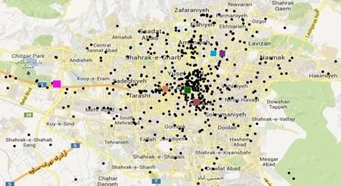
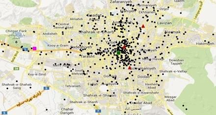
Kahfi, Tavakkoli-Moghaddam and Seyed-Hosseni

 Second objective

 First objective

 Figure 6. Pareto fronts of two meta-heiristics

The MODA Pareto front is demonstrated in Figure 6. However, the MODA Pareto front is not sufficient for the
determination of cash supply centers in the bank case study. Selecting the best and most efficient final solution depends
on the priorities of the decision-makers. Therefore, the bank experts have surveyed the Pareto front of the case study.
They have selected a solution based on bank rules. The most important of these rules are as follows:
 1) Availability of the estate, security issues and traffic in the proposed area of the solution.
 2) Minimum waiting time as second objective in the solution.
 3) Existence of at least four supply centers in the solution based on the bank experts experiences.
 As an example, two solutions from the Pareto front (Figure 6) obtained from the MODA are shown in Figure 7.
Although solution (a) has the minimum cost between Pareto front and there are at least four supply centers; however,
solution (b) has all of conditions and is selected as the best solution by bank experts.

 Figure 7. (a) Sample of Pareto front

 Int J Supply Oper Manage (IJSOM), Vol.8, No.1 14

Robust Bi-Objective Location-Arc Routing Problem with Time Windows: a Case Study of an Iranian Bank

 Figure 7. (b) Sample of Pareto front

7. Conclusion and future research
To cope with the issue of the location of cash supply centers that servicing to bank branches under uncertain demand, this
paper proposed a new mixed-integer linear programming model for a bi-objective and multi-period Location-Arc Routing
Problems (LARP) with time windows. To the best of our knowledge, for the first time, the time windows were modeled
in the LARP with a condition of converting the required arc with time windows to a deadheading arc without time
windows after service. Also, the model forces the vehicle to service multiple required arc with the minimum deadheading
arc in route. The case study was a node-routing problem with the closest nodes that were converted to the model of the
LARP with a reduced dimension. The proposed model was solved by the Multi-Objective Dragonfly Algorithm (MODA)
and Non-dominated Sorting Genetic Algorithm (NSGA-II), in which the MODA based on the multi-objective metrics has
better performance. The approach proposed by Bertsimas and Sim was used due to the uncertainty in demand. The
computational results showed that the robust model under the realization outperforms the deterministic model in terms of
the mean and standard deviation. However, the deterministic model with nominal data had better objective function
values. In this case study to determine the cash supply centers, bank experts surveyed the MODA Pareto front based on
the availability of the estate, security issues, minimum waiting time, etc. Finally, five cash supply centers in Tehran were
selected. Considering other features for developing the model of the LARP, investigating the uncertainty in other model
parameters and solving the model with an exact method can be a good direction for future research. Another direction is
to consider the risk of cash-in-transit for the bank case study.

References
Albareda-Sambola M. (2015). Location-routing and location-arc routing. Location science, Springer, Cham.
Amini A., Tavakkoli-Moghaddam R. and Ebrahimnejad S. (2017). Scenario-Based Location Arc Routing Problems:
Introducing Mathematical Models. In International Conference on Management Science and Engineering Management
(pp. 511-521). Springer, Cham.
Amini A., Tavakkoli-Moghaddam R. and Ebrahimnejad S. (2019). A bi-objective transportation-location arc routing
problem, Transportation Letters, Vol. 12, pp. 623-637.
Armas J., Ferrer A., Juan A.A. and Lalla-Ruiz E. (2018). Modeling and solving the non-smooth arc routing problem with
realistic soft constraints. Expert systems with applications, Vol. 98, pp.205-220.
Babaee Tirkolaee, E., Goli A.R. , Pahlevan M. and Malekalipour Kordestanizadeh R. (2019). A robust bi-objective multi-
trip periodic capacitated arc routing problem for urban waste collection using a multi-objective invasive weed
optimization. Waste Management & Research, Vol. 37, No. 11, pp. 1089-1101.

 Int J Supply Oper Manage (IJSOM), Vol.8, No.1 15

Kahfi, Tavakkoli-Moghaddam and Seyed-Hosseni

Babaee Tirkolaee E., Mahdavi I. and Seyyed Esfahani M.M. (2018). A robust periodic capacitated arc routing problem
for urban waste collection considering drivers and crew’s working time. Waste Management, Vol. 76, pp.138-146.
Babaee Tirkolaee E., Mahdavi I., Seyyed Esfahani M.M. and Weber G.W. (2020). A hybrid augmented ant colony
optimization for the multi-trip capacitated arc routing problem under fuzzy demands for urban solid waste
management. Waste Management & Research, Vol. 38, No. 2, pp. 156-172.
Ben-Tal A. and Nemirovski A. (1998). Robust convex optimization. Mathematics of operations research, Vol. 23, No.
4, pp. 769-805.
Bertsimas D. and Sim M. (2004). The price of robustness. Operations research, Vol. 52, No. 1, pp. 35-53.
Black D., Eglese R. and Wøhlk S. (2013). The time-dependent prize-collecting arc routing problem. Computers &
Operations Research, Vol. 40, No. 2, pp. 526-535.
Çetinkaya C., Gökçen H. and Karaoğlan İ. (2018). The location routing problem with arc time windows for terror regions:
a mixed integer formulation. Journal of Industrial and Production Engineering, p. 1-10.
Çetinkaya C., Karaoglan I. and Gökçen H. (2013). Two-stage vehicle routing problem with arc time windows: A mixed
integer programming formulation and a heuristic approach. European Journal of Operational Research, Vol. 230, No. 3,
pp. 539-550.
Collette Y., Siarry P. (2003). Multi-objective optimization: principles and case studies, New York: Springer.
Deb K., Pratap A., Agarwal, S. and Meyarivan T. (2002). A fast and elitist multiobjective genetic algorithm: NSGA-II.
IEEE Transactions on evolutionary computation, Vol. 6, No. 2, pp. 182-197.
Doulabi S.H.H. and Seifi A. (2013). Lower and upper bounds for location-arc routing problems with vehicle capacity
constraints. European Journal of Operational Research, Vol. 224, No. 1, pp. 189-208.
Essink E. and Wagelmans A. (2015). A comparison of 3 metaheuristics for the location-arc routing problem.
DOI: 10.13140/RG.2.1.2781.0649.
Fernández E. Laporte G. and Rodríguez-Pereira J. (2019). Exact Solution of Several Families of Location-Arc Routing
Problems. transportation science Articles in Advance, Vol. 53, No. 5, pp.1313-1333.
Fazli-Khalaf M., Fathollahzadeh K., Mollaei A., Naderi B. and Mohammadi M. (2019). A robust possibilistic
programming model for water allocation problem. RAIRO-Operations Research, Vol. 53, No. 1, pp.323-338.
Fazli-Khalaf M. and Hamidieh A. (2017). A robust reliable forward-reverse supply chain network design model under
parameter and disruption uncertainties. International Journal of Engineering-Transactions B: Applications, Vol. 30, No.
8, pp.1160-1169.
Ghiani G., Improta G. and Laporte G. (2001). The capacitated arc routing problem with intermediate facilities. Networks,
Vol. 37, No. 3, pp. 134-143. Golden B.L. and Wong R. T. (1981). Capacitated arc routing problems. Networks, Vol. 11,
No. 3, pp. 305-315.
Hamidieh A., Arshadikhamseh A. and Fazli-Khalaf M. (2018). A robust reliable closed loop supply chain network design
under uncertainty: A case study in equipment training centers. International Journal of Engineering-Transactions A:
Basics, Vol. 31, No. 4, pp.648-658.
Huber S. (2016). Strategic decision support for the bi-objective location-arc routing problem. Paper presented at the
Proceedings of the 2016 49th Hawaii International Conference on System Sciences (HICSS).
Javanmardi A. and Hafezalkotob A. (2018). Presenting a multi-objective locating-routing-arc model with collaborative
approach (A food distribution case study). Journal of Industrial and Systems Engineering, Vol. 11, special issue on game
theory applications, pp. 144-163.
kahfi A., seyedhosseini S.M. and Tavakkoli-Moghaddam R. (2020). A robust optimization approach for a multi-period
location-arc routing problem with time windows: a case study of a bank. International Journal of Non-linear Analysis
and Applications, Accepted for publication.
Khajepour A., Sheikhmohammady M. and Nikbakhsh E. (2020). Field path planning using capacitated arc routing
problem. Computers and Electronics in Agriculture, Vol. 173, No. 105401, pp. 1-10.
Kirlik G. and Sipahioglu A. (2012). Capacitated arc routing problem with deadheading demands. Computers &
Operations Research, Vol. 39, No. 10, pp. 2380-2394.

 Int J Supply Oper Manage (IJSOM), Vol.8, No.1 16

Robust Bi-Objective Location-Arc Routing Problem with Time Windows: a Case Study of an Iranian Bank

Lacomme P., Prins C. and Ramdane-Cherif W. (2004). Competitive memetic algorithms for arc routing problems. Annals
of Operations Research, Vol. 131, No. 1-4, pp. 159-185.
Laporte G., Nickel S., and da Gama F. S. (2015). Location science. Springer , Cham.
Levy L., and Bodin L. (1989). The arc oriented location routing problem. INFOR: Information Systems and Operational
Research, Vol. 27, No.1, 74-94.
Liu M., Singh H.K. and Ray T. (2014). Application specific instance generator and a memetic algorithm for capacitated
arc routing problems. Transportation Research Part C: Emerging Technologies, Vol. 43, pp. 249-266.
Lopes R.B., Plastria F., Ferreira C. and Santos B.S. (2014). Location-arc routing problem: Heuristic approaches and test
instances. Computers & Operations Research, Vol. 43, pp. 309-317.
Lystlund L. and Wøhlk S. (2012), The service-time restricted capacitated arc routing problem. Working paper.
Macedo R., Alves C., de Carvalho J.V., Clautiaux F. and Hanafi S. (2011). Solving the vehicle routing problem with time
windows and multiple routes exactly using a pseudo-polynomial model. European Journal of Operational Research, Vol.
214, No. 3, pp. 536-545.
Mirjalili S. (2016). Dragonfly algorithm: a new meta-heuristic optimization technique for solving single-objective,
discrete, and multi-objective problems. Neural Computing and Applications, Vol. 27, No. 4, p. 1053-1073.
Mirzaei-Khafri S., Bashiri M., Soltani R. and Khalilzadeh M. (2019). A Mathematical Model For The Capacitated
Location-Arc Routing Problem With Deadlines And Heterogeneous Fleet. Transport, Vol. 34, No. 6, pp. 692–707.
Mirzaei-Khafri S., Bashiri M., Soltani R. and Khalilzadeh M., (2020). A robust optimization model for a location-arc
routing problem with demand uncertainty, International Journal of Industrial Engineering: Theory, Applications and
Practic, Vol. 27, No. (2).
Pavlis N.E., Moschuris S.J. and Laios L.G. (2018). Supply management performance and cash conversion
cycle. International Journal of Supply and Operations Management, Vol. 5, No. 2, pp.107-121.
Riquelme-Rodríguez J.P., Gamache, M. and Langevin A. (2016). Location arc routing problem with inventory constraints.
Computers & Operations Research, Vol. 76, pp. 84-94.
Soyster A.L. (1973). Convex programming with set-inclusive constraints and applications to inexact linear programming.
Operations research, Vol. 21, No. 5, pp. 1154-1157.
Tavakkoli-Moghaddam R., Amini A., Ebrahimnejad S. (2018). A new mathematical model for a multi-product location-
arc routing problem. in: Optimization and Applications (ICOA), 2018 4th International Conference on, IEEE.
Teimoori S., Khademi Zare H. and Fallah Nezhad M.S. (2014). Location-routing problem with fuzzy time windows and
traffic time. International Journal of Supply and Operations Management, Vol. 1, No. 1, pp.38-53.
Vansteenwegen P., Souffriau W. and Sörensen K. (2010). Solving the mobile mapping van problem: A hybrid
metaheuristic for capacitated arc routing with soft time windows. Computers & operations research, Vol. 37, No. 11, pp.
1870-1876.

 Int J Supply Oper Manage (IJSOM), Vol.8, No.1 17