A Fast Adaptive Speech Extraction Method using Blind Source Separation for Audio Signal Processing - IJITEE
←
→
Page content transcription
If your browser does not render page correctly, please read the page content below
International Journal of Innovative Technology and Exploring Engineering (IJITEE)
                                                                        ISSN: 2278-3075, Volume-9 Issue-4, February 2020

   A Fast Adaptive Speech Extraction Method using
      Blind Source Separation for Audio Signal
                     Processing
                               Mandli Rami Reddy, M L Ravi Chandra, Alam Siva sankar

    Abstract: The adaptive signal processing methods are used in        The ICA is an important techniques used for extraction. This
several applications like channel estimation, Noise removal and         technique works on an extension of the principal component
extraction of signals also. The methods vary on time, frequency         analysis (PCA). The PCA is a technique which optimizes
and statistical approach. In this paper, the source speech signals
are separated using different methods like FastICA,PCA and
                                                                        the covariance matrix of the data in statistics of second-
kICA. Comparison of original signal and estimated signals are           order. Hence higher order statistics can optimize ICA as
evaluated for different methods. The implementation was done in         kurtosis. This can be processed to find uncorrelated
MATLAB. The spectrogram, Negentropy and Kurtosis waveforms              components with independent components. Thus PCA
are plotted for different methods.                                      performs at the higher-order correlations in which it is
   KeyWords:      BSS, ICA, noise,          speech,    spectrogram,     extracted independently when the sources of mixture data
Negentropy, Kurtosis, statistical.                                      are insignificant.

                   I.    INTRODUCTION
The issue in Blind Source Separation (BSS) is increasing
faster by day to day usage. This issue is found similar in
other application such as, multi-path channel identification,
equalization and direction of arrival (DOA), speech
enhancement estimation and crosstalk removal in
multichannel in sensor arrays. By using this application the
higher-order statistics is improved by generating new
technique for identifying statistically independent signals in
signal modeling. The separation of source issue that is
harmful at the heart which is developed by the signal
processing and also by machine learning which is driven                             Fig. 1 The cocktail party problem.
mainly as a density estimation task. The BSS is one of the
main uses of separating the signals. The process of                     From the figure 1 found that two source signals are
separation of voice signals of people at same time called               generated from separate individuals. The two sensors are
BSS. The main problem in voice signal is the cocktail party             then recorded by microphones and later on the two source
problem. This problem is rectified by algorithm called the              signals is mixed. Thus by using this process the original
independent component analysis (ICA) technique. The main                signals is recovered from the mixed signals.
process technique used in this method is to detect the sound
with single object in various sound environments. Figure. 1                          II.    LITERATURE SURVEY
shows the cocktail party problem which is the best example
of two vocal signals. The voices have two types of source               Parra et al, (2000) performs optimization technique using
that are recorded from two independent source signals.                  algorithm utility for automatic speech recognition. This
Hence the problems are carried out and solved by extracting             methodology simulates the acoustic signal that is recorded
the original signals using independent component analysis               in a reverberant environment. The recorded signals are the
(ICA) technique.                                                        sums of differently convolved sources. Thus the process
                                                                        identifies the unknown channel and optimizes the channel.
                                                                        Y. Yang et al, (2011) introduce a temporal predictability
                                                                        based Blind Source Separation (BSS). This method used to
                                                                        separate the signal from the mixed one. Thus the simulation
                                                                        shows that the signals are separated to get individual noise
                                                                        source signals. Zhinong Li et al, (2008) compares the
Revised Manuscript Received on January 22, 2020.                        machine faults in linear BSS method. The source separation
* Correspondence Author                                                 method is presented which is based on linear BSS. If the
   Mandli Rami Reddy*, ECE Department, Srinivasa Ramanujan Institute    machine is in nonlinear mixing source then it is effective in
of Technology, Ananthapuramu, Andhra Pradesh, India. Email:
mandliramireddy@gmail.com                                               BSS method.
   Dr M L Ravi Chandra, ECE Department, Srinivasa Ramanujan
Institute of Technology, Ananthapuramu, Andhra Pradesh, India. Email:
mlravigates@gmail.com
   Dr Alam Siva sankar, ECE Department, Srinivasa Ramanujan Institute
of Technology, Ananthapuramu, Andhra Pradesh, India. Email:
alamsivasankar1971@gmail.com

                                                                            Published By:
    Retrieval Number: B7253129219/2020©BEIESP                               Blue Eyes Intelligence Engineering
    DOI: 10.35940/ijitee.B7253.029420                               727     & Sciences Publication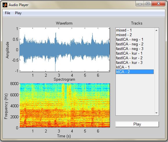
A Fast Adaptive Speech Extraction Method using Blind Source Separation for Audio Signal Processing
Thus the result is based on the separation of source correlated signals. Instantaneous BSS and Convolutive BSS
signals.S. Van Vaerenbergh and I. Santamaria (2006) are the two problems that can simplify residual signals by
describe the different nonlinearities system. This system cost function. Thus the technique compares the simulation
inverts the linear BSS which is based on clustering approach and undergoes the separation process to extract temporal
to solve problems in underdetermined post nonlinear blind structure in residual part of source signals. Tao Xu and
source separation (PNL BSS). Thus the method transforms Wenwu Wang (2009) presented K-means clustering
the nonlinear mixture component to solve undetermined algorithm to estimate unknown mixing matrix from audio
BSS problem. mixture. The separation of audio signals occur some
H. Sawada et al, (2007) introduced a blind source separation problem while address the sparse signal representation. The
(BSS) for optimizing the group frequency components. This algorithm is processed under two stages K-means clustering
method analysis ICA results for all estimation sensors for algorithm and conventional approaches. Thus the method
each source. Thus the process shows the effective separation gives better performance by comparing recent sparse
in several sources that are configured in low moderate. Bin representation approach.
Zhao et al, (2005) discussed a novel blind separation method
to determine the separated signals. At the receiver end the III. BACKGROUND METHODOLOGY
signals separation numbered to separate when direction-of-
3.1. PRINCIPAL COMPONENT ANALYSIS
arrival (DOA) is obtained. Thus the signal is separated by
the individual communication signals on source separation. The principal component analysis (PCA) is used to estimate
O. Shifeng et al, (2009) presented a novel variable step size the average value in sample. This technique consist of
algorithm to restructure. The performance index has been observed vector x to remove its mean. After the process of
restructured nonlinear based algorithm for updating rule of removal the vector will transform into a new vector. Some
step-size. This algorithm is used by adopting an auxiliary of the possibilities of vector are lower dimension whose
separation system. Thus the algorithm performs the steady elements are uncorrelated with each other. Hence the
state in both stationary and non-stationary system. Qi Lv process is carried out by evaluating the covariance matrix by
and Xian-Da Zhang (2006) simulate the speech signal using Eigen value decomposition which is found by the linear
Blind source separation (BSS) to validate the higher transformation. Thus the covariance matrix CX with a zero-
applications. In this simulation BSS is implemented without mean vector x is shown in equation (1).
prior assumption on the number of sources. Hence C Cx E{XX T } EDET (1)
prototypes algorithm is used as the new type of BSS method
to estimate the mixing matrix. Where,
K. J. Faller et al, (2017) investigate source separation
algorithms to improve intelligibility of speech. This method E (e1, e2….en) = CX
can enhance the spatial hearing of hearing aids. Thus the Cx represents the eigenvectors in orthogonal matrix.
BSS algorithm will modify the speech source that is
simulated as spatial audio. Y. Zhang and S. A. Kassam D=Diag (1,2,….n) CX in Diagonal matrix of Eigen
(2010) discuss complex blind source separation. This value.
algorithm performs via EASI system. The process is carried
out with the QAM signal which is separated. This technique Whitening can be shown as
is based on magnitude-phase which represents the complex Z P* X (2)
signals and circularly symmetric source. Z. Li et al, (2010)
presented the whitening and non-linear de-correlation based Where, P denotes the whitening matrix and Z denotes white
Blind source separation algorithm. The ICA is also be used new matrix.
in this to take results in neural network and signal
processing. Thus the method simulated and analyzed using P is represents as;
BBS algorithm and the corresponding result gives better P D 0.5 E T (3)
convergence speed and steady-state error. Yoshihiro Sakai et
al, (2007) discuss the BSS algorithm to improve the 3.2. ICA
convergence rate. This methodology uses the blind signal
The signals are varies from time and it is
separation circuit to reduce failure during double-talk in the
represented as, si = {si1; si2; ...; siN}, the number of time
echo canceller. Thus the circuit describes the constitution
steps is denoted by N and sij is the amplitude of the signal, si
method to get improve characteristic of blind signal
at the jth time. Given two independent source signals s1 =
separation.
{s11; s12; ...; s1N} and s2 = {s21; s22; ...; s2N} (see Fig. 1). Both
J. Ma and X. Zhang (2008) presented blind
signals are given by;
separation algorithm to get instantaneous linear mixture
S ( S , S ,...., S1N )
signals for low computational complexity. This method will S 1 11 12 (4)
characterize based on Signal Noise Ratio (SNR) at maximal S 2 ( S 21 , S 22 ,...., S 2 N )
condition. The source signals and noises have same
eigenvalue (GE) problem. Thus the method is compared Where, S R P N denotes the space and also defines the
with the algorithm to have effective low complexity in
source signal. The source
computation. B. Xia and H. Xie (2007) discuss two main
signal indicates p.
problems that affect blind source separation in temporal
Published By:
Retrieval Number: B7253129219/2020©BEIESP Blue Eyes Intelligence Engineering
DOI: 10.35940/ijitee.B7253.029420 728 & Sciences Publication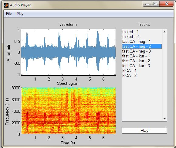
International Journal of Innovative Technology and Exploring Engineering (IJITEE)
ISSN: 2278-3075, Volume-9 Issue-4, February 2020
Both S1 and S2 are the mixed source signals as non-Gaussian random variable then the kurtosis is zero.
X 1 a *1 b * s 2 . Here a and b are the mixing Here a particular kurtosis value can be either positive or
negative. The positive value is called Super-gaussian and
coefficients in x1. Hence the mixture x1 is the weighted as
negative value is called Sub-gaussian. Super-gaussian
sum of the two source signals. X2 mixture is repeated as the
random variables and sub-gaussian random variables both
same process and the distance between the source signals
have a spiky probability density function and flat probability
and the sensing device is changed for measuring. The
density function.
mathematical representation is shown as
X 2 c * S1 d * S 2 . Where, c and d are mixed 3.2.2 Negentropy
coefficients. The mixed coefficients are different from Negentropy is another main technique used to measure the
coefficients c and d due to sensing devices that has both non-gaussianity. The Negentropy works in different entropy
signals in different locations. Thus the source signals are based on the information theoretic quantity. The entropy
measured with each sensor in a different mixture. Hence the means that it can be interpreted on random variable which is
corresponding output in source signal has different impact the basic concept of information theory as the degree of
which is represented as follows: information. Entropy can observe the random variable that is
X aS bS2 a b S1 unpredictable and unstructured in the larger entropy. This
X 1 1 As (5)
X 2 cS1 dS2 c d S 2
technique is closely related to the coding length of the
random variable.
Here X R n N denotes the mixture signals. Where n is the 3.3. FastICA:
number of mixtures. Thus (figure 1) the mixing coefficients This method is highly efficient for computing the signal by
such as a; b; c, and d are utilized for transforming linearly using FastICA algorithm. The FastICA is used to estimate
ICA performance which uses a fixed-point iteration scheme
source signals. This source signals are mixed to space
that are found. For ICA the method could be 10-100 times
signals S in X space, S →X : X = AS, where A R n P is the faster than conventional gradient descent method. The
mixing coefficients matrix: advantage of FastICA algorithm is that it can be used to
perform projection pursuit as well as providing a general-
A ac db (6) purpose data analysis method.
The Steps involves Fast ICA algorithm:
1. It makes the mixed data available at zero mean.
Properties of Mixed Signals: 2. Whiten the data.
1. Independence: If signals are shared between the 3. The initial weight vector w of unit norm is taken.
mixtures then it is independent when the source wnorm w (8)
signals are independent to mixture signals. w
2. Gaussianity: The gaussianity is a process of Let
mixing signals in histogram that are bell shaped.
wnew E{mi g (wT mi )} E{mi g ' (wT mi )}w (9)
This can be used for searching for non-Gaussian
signals within mixture signals. The signals are The equation shows the basic weight update, where g is the
extracted independently when they must be non- contrast function.
Gaussian. Hence the signals are estimated wnew
Let wnew (10)
independently when they have fundamental wnew
restriction in ICA.
Thus the normalization step makes the new w as unit norm
3. Complexity: This is more complex than source
and it will update in each iteration. Compare wnew with the
signals which is shown from the previous example
old vector, if converged than move ahead, if not go to step 4.
of mixed signals. The extracted signals are
independent and they are non-Gaussian histograms
IV. PROPOSED METHODOLOGY
with these signals which represent source signals.
4.1. KERNEL INDEPENDENT COMPONENT
3.2.1. MEASURING NON GAUSSIANITY ANALYSIS
Kurtosis: The Kernel ICA (KICA) is an algorithm that
The Kurtosis is used to measure non-Gaussianity by process non-linear transformation by combining KPCA with
the absolute value of kurtosis. This theorem has central limit ICA. The ICA deal with the sample data using basic idea of
which is strong measure signal with traditional higher order the KICA which is mapped to high dimension feature space
statistics that uses kurtosis independent. The kurtosis is by using nonlinear characteristics. This method confirms to
defined by zero-mean random variable v given as; Mercer condition. In this technique the KPCA uses the
Kurt(v) E{v 4 } 3( E{v 2 }) 2 (7) linear principle component analysis to deal with the sample
4 data for mapping high dimension feature using a nonlinear
Where E{v } =Fourth moment of v, and E{v 2 } mapping transformation.
=Second moment of v.
4 2 2
Here, the E{v } equals 3( E{v }) where v is the
Gaussian random variable. From the equation (7) if v is a
Published By:
Retrieval Number: B7253129219/2020©BEIESP Blue Eyes Intelligence Engineering
DOI: 10.35940/ijitee.B7253.029420 729 & Sciences Publication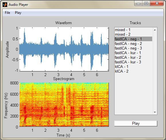
A Fast Adaptive Speech Extraction Method using Blind Source Separation for Audio Signal Processing
Common use of kernel functions;
1. The Radial Basics Gaussian Function is given in Principal Components
5
equation (11) which defines infinite dimension in
feature space.
Zpca(1,:)
x x' 2 0
k ( x, x' ) exp (11)
2 2
-5
0 10 20 30 40 50 60 70 80 90 100
2. Equation (12) represents the Polynomial Kernel
6
Function defines finite dimensions
4
k ( x, y) (( x. y) c) 2 (12)
Zpca(2,:)
2
0
V. RESULT AND DISCUSSION -2
-4
Thus the experiment shows the uses of source speech 0 10 20 30 40 50 60 70 80 90 100
signals. Different methodology of separations are mixed and
then used for evaluation. The experiment is performed in Fig 3(a): Principle components of source signal
MATLAB platform and the corresponding results taken
2D PCA approximation of 3D data
using BSS algorithms that are FastICA, PCA and KICA. 10
The waveform and spectrogram of source signals is shown 5
Z(1,:)
in figure (2). 0
-5
Source 1
0 10 20 30 40 50 60 70 80 90 100
1
0.8
12
0.6 Z(2,:)
0.4
0.2
10
0
-0.2
8
-0.4
0 10 20 30 40 50 60 70 80 90 100
-0.6
-0.8 15
-1
0 0.5 1 1.5 2 2.5 3 3.5 4 4.5 5
Z
10
Z(3,:)
4
x 10
Zr
5
spectogram
1 0
0.9
0 10 20 30 40 50 60 70 80 90 100
0.8
0.7
0.6
Fig 3 (b): original and estimated signal
Frequency
0.5
0.4
0.3
0.2
0.1
0
0.5 1 1.5 2
Time 4
x 10
Source 2
1
0.8
0.6
0.4
0.2
0
-0.2
-0.4
-0.6
-0.8
0 0.5 1 1.5 2 2.5 3 3.5 4 4.5 5
4
x 10
Source 2
1
0.8
0.6
0.4
0.2
0
-0.2
-0.4
-0.6
-0.8
0 0.5 1 1.5 2 2.5 3 3.5 4 4.5 5
4
x 10
spectogram
1
0.9
0.8
0.7
0.6
Frequency
0.5
0.4
0.3
0.2
0.1
0
0.5 1 1.5 2
Time 4
x 10
Fig 2. Source signal and its spectrogram
The corresponding output waveform of principle component
analysis is shown in figure (3). Hence, fig 3(a) represents
principle components of signal and comparison of original
signal and estimated PCA signal is shown in fig 3(b).
Published By:
Retrieval Number: B7253129219/2020©BEIESP Blue Eyes Intelligence Engineering
DOI: 10.35940/ijitee.B7253.029420 730 & Sciences Publication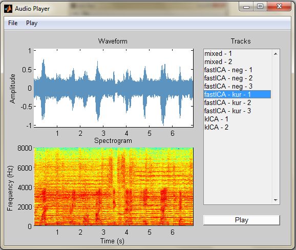
International Journal of Innovative Technology and Exploring Engineering (IJITEE)
ISSN: 2278-3075, Volume-9 Issue-4, February 2020
Fig 4: waveform and its Spectrogram of mixed signals
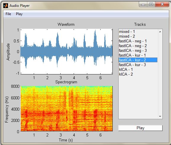
Here the waveform and spectrogram of mixed signals is
shown above in figure (4). Figure 5 represents the signals
that are processed using FastICA based on Negentropy and
Kurtosis components.
Fig 5(b): Kurtosis waveforms using FastICA
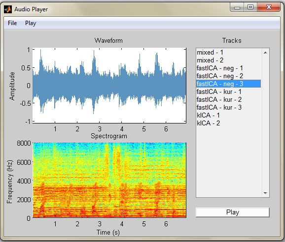
The KICA output waveform and its spectrogram is shown in
figure (6).
Fig 5(a): Negentropy waveforms using FastICA
Published By:
Retrieval Number: B7253129219/2020©BEIESP Blue Eyes Intelligence Engineering
DOI: 10.35940/ijitee.B7253.029420 731 & Sciences Publication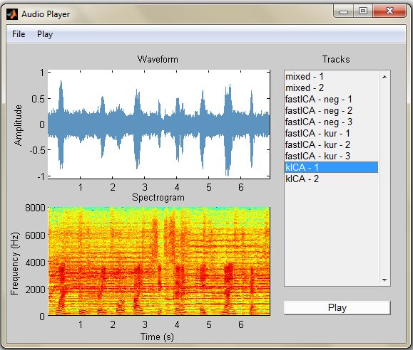
A Fast Adaptive Speech Extraction Method using Blind Source Separation for Audio Signal Processing

                                                                              8.    Qi Lv and Xian-Da Zhang, "A unified method for blind separation of
                                                                                    sparse sources with unknown source number," in IEEE Signal
                                                                                    Processing Letters, vol. 13, no. 1, pp. 49-51, Jan. 2006.
                                                                              9.    K. J. Faller, J. Riddley and E. Grubbs, "Automatic blind source
                                                                                    separation of speech sources in an auditory scene," 2017 51st Asilomar
                                                                                    Conference on Signals, Systems, and Computers, Pacific Grove, CA,
                                                                                    2017, pp. 248-250.
                                                                              10.   Y. Zhang and S. A. Kassam, "Complex blind source separation:
                                                                                    optimal nonlinearity and approximation," 2010 44th Annual
                                                                                    Conference on Information Sciences and Systems (CISS), Princeton,
                                                                                    NJ, 2010, pp. 1-6.
                                                                              11.   Z. Li, J. An, L. Sun and M. Yang, "A Blind Source Separation
                                                                                    Algorithm Based on Whitening and Non-linear Decorrelation," 2010
                                                                                    Second International Conference on Computer Modeling and
                                                                                    Simulation, Sanya, Hainan, 2010, pp. 443-447.
                                                                              12.   Yoshihiro Sakai, Kota Takahashi and Wataru Mitsuhashi, "An
                                                                                    alogrithmic study on blind source separation for preprocessing of an
                                                                                    acoustic echo canceller," SICE Annual Conference 2007, Takamatsu,
                                                                                    2007, pp. 1400-1405.
     Fig 6: Estimated waveform and Spectrogram using                          13.   J. Ma and X. Zhang, "Blind Source Separation Algorithm Based on
                           kICA                                                     Maximum Signal Noise Ratio," 2008 First International Conference on
                                                                                    Intelligent Networks and Intelligent Systems, Wuhan, 2008, pp. 625-
                                                                                    628.
  Table 1: Mean Square Error(MSE) for PCA, FastICA                            14.   B. Xia and H. Xie, "Blind Source Separation of Temporal Correlated
                       and kICA                                                     Signals," 2007 Third International IEEE Conference on Signal-Image
                                      MSE                                           Technologies and Internet-Based System, Shanghai, 2007, pp. 549-
                                                                                    555.
   PCA                               0.0718                                   15.   Tao Xu and Wenwu Wang, "A compressed sensing approach for
      FastICA (negentropy)           0.0296                                         underdetermined blind audio source separation with sparse
   FastICA (kurtosis)                0.0292                                         representation," 2009 IEEE/SP 15th Workshop on Statistical Signal
                                                                                    Processing, Cardiff, 2009, pp. 493-496.
   kICA                              0.0254                                   16.   A. Siva Sankar, Dr.T. Jayachandra Prasad, Dr.M.N.Giriprasad, “LSB
Table 1 shows the Mean square error (MSE) for different                             based Lossless Digital Image Watermarking using Polynomials in
technique.                                                                          Spatial Domain for DRM”, International Journal of Computer
                                                                                    Association (IJCA), New York, USA, ISBN: 978-93-80747-76-3, No.
                                                                                    13, pp. 18-23, 2011.
                     VI.     CONCLUSION                                             www.ijcaonline.org/proceedings/icwet/number13
                                                                              17.   Mandli Rami Reddy, T. Keerthi Priya, k. Prasanth, S.Ravindrakumar
The paper presented the efficiency of the blind source                              “Robust Adaptive Estimator using Evolutional algorithm for Noise
separation (BSS) method on signal separation process. The                           Cancellation In Multichannel System “ Chapter DOI.: 10.1007/978-
                                                                                    981-13-8942-9_55
basic idea is the separation of sources which are statistically
independent. The methods are complex in nature and
                                                                                                      AUTHORS PROFILE
execution but found efficient. Several methods like FastICA,
PCA and kICA are implemented in MATLAB. The methods                                               M.Rami Reddy, received the bachelor degree in
                                                                                                 Electronics and communication engineering from Sri
are tested using sources of speech signals. The spectrogram,                                     Venkateswara College of engineering and technology
Negentropy and Kurtosis waveforms are plotted for different                                      (SVCET) Chittoor in 2005 and received the post
methods.                                                                                         graduate in communication and signal processing from
                                                                                                 G.Pulla Reddy engineering college (GPREC), Kurnool in
                                                                                                 2010. He is currently working as Assistant professor in
REFERENCES                                                                    the srinivasa ramanujan institute of technology (SRIT). His research
                                                                              activities are in adaptive signal processing with a particular interest sub
1.   Parra, Lucas C. and Clay D. Spence. “Convolutive blind separation of     band least mean square algorithm. He handled various subjects for post
     non-stationary sources.” IEEE Trans. Speech and Audio                    graduate students. He is having 13 years of teaching experience. He has
     Processing, Vol.8, No.3, pp.320-327,2000.
                                                                              published 9 international papers and four national paper. He is life member
2.   Y. Yang, Z. Li, X. Wang and D. Zhang, "Noise source separation           of ISTE, IEI, IETE.
     based on the blind source separation," 2011 Chinese Control and              .
     Decision Conference (CCDC), Mianyang, 2011, pp. 2236-2240.
3.   Zhinong Li, Yudong Zeng, Tao Fan, Yaping Lv and Jinge Ren,
                                                                                                      Dr.M.L.Ravi Chandra, obtained his B.Tech degree
     "Source Separation method of Machine Faults Based on Post-
     Nonlinear Blind Source Separation," 2008 7th World Congress on                                  in Electronics and Communication Engineering, from
     Intelligent Control and Automation, Chongqing, 2008, pp. 1786-1789.                             KSRMCE, Affiliated to S.V. University and Master
4.   S. Van Vaerenbergh and I. Santamaria, "A spectral clustering approach                           of Technology in Digital Systems and Computer
     to underdetermined postnonlinear blind source separation of sparse                              Electronics from JNTUACE,Anantapur, A.P. India.
     sources," in IEEE Transactions on Neural Networks, vol. 17, no. 3, pp.                          He obtained his Ph.D. Degree from JNTUHCE,
     811-814, May 2006.                                                                              Hyderabad, Telanagana,India. He worked at various
5.   H. Sawada, S. Araki, R. Mukai and S. Makino, "Grouping Separated
                                                                                                    engineering colleges in Andhra Pradesh and
     Frequency Components by Estimating Propagation Model Parameters
     in Frequency-Domain Blind Source Separation," in IEEE Transactions       Telangana as Assistant Professor, Associate Professor, Professor and Head
     on Audio, Speech, and Language Processing, vol. 15, no. 5, pp. 1592-     of the Department. Presently he is working as a Professor and Head for
     1604, July 2007.                                                         ECE Department at Srinivasa Ramanujan Institute of Technology,
6.   Bin Zhao, Jun-An Yang and Min Zhang, "Research on blind source           Anantapur, A.P., India from December,2015 to till date. He is having 20
     separation and blind beamforming," 2005 International Conference on      years of teaching experience. He has 15 technical publications in
     Machine Learning and Cybernetics, Guangzhou, China, 2005, pp.            International Journals and 7 publications in International Conferences. He
     4389-4393 Vol. 7.
                                                                              is a life member of IE(I) and Member of IEEE.
7.   O. Shifeng, G. Ying, J. Gang and Z. Xuehui, "Variable Step Size
     Algorithm for Blind Source Separation Using a Combination of Two
     Adaptive Separation Systems," 2009 Fifth International Conference on
     Natural Computation, Tianjin, 2009, pp. 649-652.

                                                                                    Published By:
     Retrieval Number: B7253129219/2020©BEIESP                                      Blue Eyes Intelligence Engineering
     DOI: 10.35940/ijitee.B7253.029420                                    732       & Sciences Publication
International Journal of Innovative Technology and Exploring Engineering (IJITEE)
                                                                            ISSN: 2278-3075, Volume-9 Issue-4, February 2020

                     Alam Siva Sankar,          obtained his Diploma in
                     Electronics and communication Engineering at S.V.
                     Government Polytechnic, Tirupati, A.P. and obtained
                     his AMIE in Electronics and Communication Engg.,
                     from The Institution of Engineers (India), Kolkata 700
                     020 , and Master of Technology degree in Digital
                     Electronics and Advanced Communication from
                     Manipal Institute of Technology(MIT), Manipal –
576104, Karnataka state, India. He obtained his Ph.D. Degree (Digital
Rights Management/Digital Image Watermarking) in ECE from
JNTUACE, Anantapur, A.P., India. He worked in Hindustan College of
Engineering, Chennai from Jun, 1997 to April, 2002 as a lecturer. He
worked as a Lecturer in ECE Dept. in Anand Institute of Higher
Technology, Chennai, from Sep, 2003 to June, 2004. He worked in Gokula
Krishna College of Engineering, sullurpet from July, 2004 to April, 2012 in
various positions such as Assistant Professor and HOD, Associate Professor
and HOD and Professor and HOD. He worked in Priyadarshini College of
Engineering, Sullurpet from May, 2012 to April, 2015 as a Professor and
Principal. Worked in Priyadarshini Institute of Technology, Tirupati from
May, 2015 to March, 2016 as a Professor and Academic Dean. Worked in
KMM institute of Technology and Science, Tirupati, from April, 2016 to
June, 2018 as a Professor and Principal. Presently working as a Professor in
ECE Dept. in Srinivasa Ramanujan Institute of Technology, Anantapur,
A.P., India to till date. He is having more than 20 years of teaching
experience and has more than 16 technical publications in International
Journals and Conferences. He is a life member of ISTE (India), Associate
Member of Institution of Engineers (India). He is a Member of IEEE.

                                                                                 Published By:
     Retrieval Number: B7253129219/2020©BEIESP                                   Blue Eyes Intelligence Engineering
     DOI: 10.35940/ijitee.B7253.029420                                     733   & Sciences Publication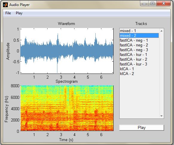
You can also read