Exhaust Gas Analysis and Parametric Study of Ethanol Blended Gasoline Fuel in Spark Ignition Engine
←
→
Page content transcription
If your browser does not render page correctly, please read the page content below
American Journal of Engineering Research (AJER)                                                           2013

                                     American Journal of Engineering Research (AJER)
                                                e-ISSN : 2320-0847 p-ISSN : 2320-0936
                                                       Volume-02, Issue-07, pp-191-201
                                                                         www.ajer.org

Research Paper                                                                                      Open Access

    Exhaust Gas Analysis and Parametric Study of Ethanol Blended
               Gasoline Fuel in Spark Ignition Engine
             Jitendra kumar1, N.A Ansari2, Vikas Verma3, Sanjeev Kumar4
1
  M.Tech Scholar, Department of Mechanical Engineering, Delhi Technological University, New Delhi-110042,
                                                    India,
 2
   Asst. Professor, Department of Mechanical Engineering, Delhi Technological University, New Delhi-110042,
                                                    India,
  3
    PhD. Scholar, Department of metallurgical and materials engineering, IIT Roorkee , Uttarakhand, -247667,
                                                     India
      4
        Asst. Professor, Department of Mechanical Engineering, KIMT, U.P Moradabad -244001U.P, India,

Abstract: - It is well known that the future availability of energy resources, as well as the need for reducing
CO2 emissions from the fuels used has increased the need for the utilization of regenerative fuels. This research
is done taking commercial gasoline as reference which is originally blended with 5% ethanol. Hence 5%, 10%,
15%, 20% ethanol blended with Gasoline initially was tested in SI engines. Physical properties relevant to the
fuel were determined for the four blends of gasoline. A four cylinder, four stroke, varying rpm, Petrol (MPFI)
engine was tested on blends containing 5%,10%,15%,20% ethanol and performance characteristics, and exhaust
emissions were evaluated. Even though higher blends can replace gasoline in a SI engine, results showed that
there is a reduction in exhaust gases, such as HC, O2, CO, CO2 and increase in Brake Thermal Efficiency on
blending. Hence we can conclude from the result that using 10% ethanol blend is most effective and we can
utilize it for further use in SI engines with little constraint on material used to sustain little increase in pressure.

Keywords: - Spark Ignition Engine, Ethanol, Brake Thermal Efficiency, Emission, Gasoline etc.

                                         I.          INTRODUCTION
          Rising fuel prices and increased oil consumption along with the lack of sustainability of oil-based fuels
have generated an interest in alternative, renewable sources of fuel for internal combustion engines, namely
alcohol-based fuels. Currently ethanol is the most widely used renewable fuel with up to 10% by volume
blended in to gasoline for regular engines or up to 85% for use in Flex-Fuel vehicles designed to run with higher
concentrations of ethanol. Ethanol can also be used as a neat fuel in spark-ignition (SI) engines or blended up to
40% with Diesel fuel for use in compression-ignition (CI) engines [1-2]. Ethanol was introduced as a
replacement for methyl tertiary butyl ether (MTBE) when it was realized that MTBE leaked onto the ground at
filling stations resulting in the contamination of large quantities of groundwater. Ethanol is biodegradable, less
detrimental to ground water, and has an octane number much higher than gasoline as well as having a positive
effect on vehicle emissions [3].There are lots of gases in the environment which are causing pollution and
greenhouse effect and the major contributor is the transport sector due to the heavy, and increasing, traffic
levels. In spite of ongoing activity to promote efficiency, the sector is still generating significant increases in
CO2 emissions. As transport levels are expected to rise, especially in developing countries, fairly drastic
political decisions may have to be taken to eradicate this problem in the future. Furthermore, the dwindling
supply of petroleum. Today, the transport sector is a major contributor to net emissions of greenhouse gases, of
which carbon dioxide is particularly important. The carbon dioxide emissions originate mainly from the use of
fossil fuels; mostly gasoline and diesel oil in road transportation systems, although some originates from other
types of fossil fuels such as natural gas and Liquefied Petroleum Gas (LPG). If international and national goals
(such as those set out in the Kyoto protocol) for reducing net emissions of carbon dioxide are to be met, the use
of fossil fuels in the transport sector has to be substantially reduced. This can be done, to some extent, by

    www.ajer.org                                                                                          Page 191
American Journal of Engineering Research (AJER) 2013
increasing the energy efficiency of engines and vehicles and thus reducing fuel consumption on a volume per
unit distance travelled basis. However, since the total transportation work load is steadily increasing such
measures will not be sufficient if we really want to reduce the emissions of carbon dioxide.
1.1 Ethanol as a Blend
In the medium term ethanol produced from grain will probably be the most important alternative fuel
for replacing gasoline and in the long term ethanol produced from cellulose might take over from grain ethanol.
Today, ethanol accounts for a substantial part of the alternative fuel market. From an international perspective,
most research up to 1990 was focused on blends of methanol and gasoline, but some studies were carried out on
ethanol-gasoline blends. Since these studies were carried out in the USA, it can be assumed that they mainly
included vehicles with efficient emission control systems, but at the same time technical features of cars in the
USA have historically differed, at least in part, from those in Sweden. It should also be noted that for a longtime
10% ethanol has been added to commercial gasoline in many parts of the world. In the US there is considerable
experience of adding higher proportions of ethanol to gasoline than those allowed by gasoline regulations in
Sweden (Europe). The primary advantage of adding a bio based alcohol to gasoline is that it reduces net CO 2
emissions but it also has other positive effects, such as increasing the octane value of the fuel and reducing the
benzene content of the exhaust gases. The use of alcohol blended gasoline and neat fuel alcohols as substitutes
for neat gasoline have become matters of interest in many countries. The International Energy Agency (IEA),
established in 1974, follows the development, and data and other experience from various trials have been
presented and discussed at symposia organized by the International Symposium on Alcohol Fuels (ISAF).
1.2 Co-products of ethanol
The co-products that results when making ethanol are dependent on the medium used to produce the
ethanol. Table 1 shows a summary of the co-products and what they are used for.
In practice, about two-thirds of each tone of grain (i.e., the starch) is converted to ethanol. The
remaining by-product is a high protein livestock feed which is particularly well suited for ruminant animals such
as cattle and sheep. This by product is also known as Distillers' Dried Grains, DDGS. The protein in this
material is utilized more efficiently in ruminant nutrition than are other high-protein feed ingredients such as
soybean meal. This by-product of ethanol production is particularly good for Canadian dairy, beef and sheep
production. It improves the competitive position globally of producers of these farm commodities. The manure
from livestock can be used as a major source of fertilizer in grain crop production. Carbon dioxide is another by-
product produced when making ethanol. Carbon dioxide, given off in great quantities during fermentation will
be collected and cleaned of any residual alcohol, compressed and sold as an industrial commodity.
II. LITERATURE SURVEY
Fikret Yuksel et.al [4] one of the major problems for the successful application of gasoline–alcohol
mixtures as a motor fuel is the realization of a stable homogeneous liquid phase. To overcome this problem, a
new carburetor was designed. With the use of this new carburetor, not only the phase problem was solved but
also the alcohol ratio in the total fuel was increased. By using ethanol–gasoline blend, the availability analysis of
a spark-ignition engine was experimentally investigated. Sixty percent ethanol and 40% gasoline blend was
exploited to test the performance, the fuel consumption, and the exhaust emissions. As a result of this study, it
was seen that a new dual fuel system could be serviceable by making simple modifications on the carburetor and
these modifications would not cause complications in the carburetor system.Ceviz M.A et al. [5] investigated
www.ajer.org Page 192American Journal of Engineering Research (AJER) 2013
the effects of using ethanol–unleaded gasoline blends on cyclic variability and emissions in a spark-ignited
engine. Results of this study showed that using ethanol–unleaded gasoline blends as a fuel decreased the
coefficient of variation in indicated mean effective pressure, and CO and HC emission concentrations, while
increased CO2 concentration up to 10vol. % ethanol in fuel blend. On the other hand, after this level of blend a
reverse effect was observed on the parameters aforementioned. The 10vol. % ethanol in fuel blend gave the best
results.Altun Sehmus et al. [6] experimentally investigated the effect of unleaded gasoline and unleaded
gasoline blended with 5% and 10% of ethanol or methanol on the performance and exhaust emissions of a
spark-ignition engine. The engine tests were performed by varying the engine speed between 1000 and 4000
rpm with 500 rpm period at three fourth throttle opening positions. The results showed that brake specific fuel
consumption increased while brake thermal efficiency, emissions of carbon monoxide (CO) and hydrocarbon
(HCs) decreased with methanol-unleaded gasoline and ethanol-unleaded gasoline blends. It was found that a
10% blend of ethanol or methanol with unleaded gasoline works well in the existing design of engine and
parameters at which engines are operating.Amit Pal et al. [7] operated a Kirloskar, four stroke, 7.35kW, twin
cylinder, DI diesel engine in dual fuel mode (with substitution of up to 75% diesel with CNG). The results of
this experiment of substituting the diesel by CNG at different loads showed significant reduction in smoke, 10
to 15 % increase in power, 10 to 15 %reduction in fuel consumption and 20 to 40 % saving in fuel cost
(considering low cost of CNG). The most exciting result was about 33% reduction in engine noise which may
prolong the engine life significantly and the consequent sound levels of giant diesel engine reduced to that of
a similarly sized gasoline engine.Hubballi P.A et al. [8] investigated experimentally the effect of Denatured
spirit (DNS) and DNS-Water blends as fuels in a four cylinder four stroke SI engine. Performance tests were
conducted to study Brake Thermal Efficiency (BThE), Brake Power (BP), Engine Torque (T) and Brake
Specific Fuel Consumption (BSFC). Exhaust emissions were also investigated for carbon monoxide (CO),
hydrocarbons (HC), oxides of nitrogen (NOx) and carbon dioxide (CO2). The results of the experiments reveled
that, both DNS and DNS95W5 as fuels increase BThE, BP, engine torque and BSFC. The CO, HC, NO x and
CO2 emissions in the exhaust decreased. The DNS and DNS95W5 as fuels produced the encouraging results in
engine performance and mitigated engine exhaust emissions.N. Seshaiah et al. [9] tested the variable
compression ratio spark ignition engine designed to run on gasoline with pure gasoline, LPG (Isobutene), and
gasoline blended with ethanol 10%, 15%, 25% and 35% by volume. Also, the gasoline mixed with kerosene at
15%, 25% and 35% by volume without any engine modifications has been tested and presented the result. Brake
thermal and volumetric efficiency variation with brake load is compared. CO and CO2 emissions have been also
compared for all tested fuels. It is observed that the LPG is a promising fuel at all loads lesser carbon monoxide
emission compared with other fuels tested. Using ethanol as a fuel additive to the mineral gasoline, (up to 30%
by volume) without any engine modification and without any loses of efficiency, it has been observed that the
petrol mixed with ethanol at 10% by volume is better at all loads and compression ratios.
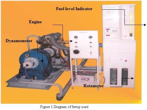
III. EXPERIMENTAL SETUP
3.1 Descriptions
The setup consists of four cylinder, four stroke, Petrol (MPFI) engine connected to eddy current type
dynamometer for loading. It is provided with necessary instruments for combustion pressure and crank-angle
measurements. These signals are interfaced to computer through engine indicator for P-V diagrams. Provision is
also made for interfacing airflow, fuel flow, temperatures and load measurement. The set up has stand-alone
panel box consisting of air box, fuel tank, manometer, fuel measuring unit, transmitters for air and fuel flow
measurements, process indicator and engine indicator. Rotameters are provided for cooling water and
calorimeter water flow measurement.
The setup enables study of engine performance for brake power, indicated power, frictional power,
BMEP, IMEP, brake thermal efficiency, indicated thermal efficiency, Mechanical efficiency, volumetric
efficiency, specific fuel consumption, A/F ratio and heat balance. Windows based Engine Performance Analysis
software package “Engine soft” is provided for online performance evaluation.
www.ajer.org Page 193American Journal of Engineering Research (AJER) 2013
3.2 Specification
Table 2.Specification
S.NO Equipment Sub-parts
1 Product Engine test setup 4 cylinder, 4 stroke, Petrol(Computerized)
2 Product code 233
3 Engine Make Maruti, Model Wagon-R MPFI, Type 4 Cylinder, 4Stroke,
Petrol (MPFI), water cooled, Power 44.5Kw at6000 rpm, Torque 59
NM at 2500rpm, stroke 61mm,bore 72mm, 1100 cc,CR 9.4:1
4 Dynamometer Type eddy current, water cooled, with loading unit
5 Propeller shaft With universal joints
6 Air box M S fabricated with orifice meter and manometer(Orifice dia 40 mm)
7 Fuel tank Capacity 15 lit with glass fuel metering column
8 Calorimeter Type Pipe in pipe
9 Piezo sensor Range 5000 PSI, with low noise cable
10 Crank angle sensor Resolution 1 Deg, Speed 5500 RPM with TDC pulse
11 Engine indicator Input Piezo sensor, crank angle sensor, No of channels
2, Communication RS232
12 Digital milivoltmeter Range 0-200mV, panel mounted
13 Temperature sensor Type RTD, PT100 and Thermocouple, Type K
14 Temperature Type two wire, Input RTD PT100, Range 0–100 Deg C,
transmitter Output 4–20 mA and Type two wire, Input
Thermocouple, Range 0–1200 Deg C, Output 4–20 mA
15 Load indicator Digital, Range 0-50 Kg, Supply 230VAC
16 Load sensor Load cell, type strain gauge, range 0-50 Kg
17 Fuel flow transmitter DP transmitter, Range 0-500 mm WC
18 Airflow transmitter Pressure transmitter, Range (-) 250 mm WC
www.ajer.org Page 194American Journal of Engineering Research (AJER) 2013
19 Rotameter Engine cooling 100-1000 LPH; Calorimeter 25-250 LPH
20 Pump Type Monoblock
21 Add on card Resolution12 bit, 8/16 input, Mounting PCI slot
22 Software “Enginesoft” Engine performance analysis software
IV. RESULT AND DISCUSSION
Gasoline Blends having 5%, 10%, 15% and 20% Ethanol is prepared. Brake thermal efficiency, HC
exhaust was plotted in parts per million, O2, CO, CO2 were plotted on volume percentage basis. These curves
are plotted firstly at no load and then at constant rpm of 3000 and 4000. The density and Lower calorific value
of blends are first calculated and then fed in the software set up configuration to get the desired results. The
results obtained were noted and then curves were plotted as shown below to have a clear understanding of the
variations of different parameters by using different blends.
4.1 No Load Test
NO LOAD
14
12
10
8
HC(PPM) 5%
6 10%
4 15%
2 20%
0
2100 2500 3000 3500 4000 4500 5000
RPM
Figure 3.HC exhaust variation with blends at different rpm.
NO LOAD
0.3
0.25
0.2
5%
O2(% VOL) 0.15
10%
0.1
15%
0.05 20%
0
2100 2500 3000 3500 4000 4500 5000
RPM
Figure 4.O2 exhaust variation with blends at different rpm.
www.ajer.org Page 195American Journal of Engineering Research (AJER) 2013
NO LOAD
0.3
0.25
0.2
5%
CO(%VOL) 0.15
0.1 10%
0.05 15%
0 20%
2100 2500 3000 3500 4000 4500
RPM
Figure 5.CO variation with blends at different rpm.
NO LOAD
15.2
15
14.8
14.6 5%
CO2(%VOL)
14.4 10%
14.2
15%
14
13.8 20%
2100 2500 3000 3500 4000 4500 5000
RPM
Figure 6.CO2 variation with blends at different rpm.
NO LOAD
30.00
25.00
20.00
5%
BThE(%) 15.00
10%
10.00
15%
5.00 20%
0.00
2100 2500 3000 3500 4000 4500 5000
RPM
www.ajer.org Page 196American Journal of Engineering Research (AJER) 2013
Figure 7.Brake Thermal efficiency variations with blends at different rpm.
At no Load conditions some points are clear which are given below.
HC emission decreases as blending increases up to 4000 rpm with respect to E5 and is lowest at 2500
rpm. For 10% blend HC emission reduces by 23.08% at 2100 rpm in comparison to commercial
Gasoline.
O2 Percentage increases as blending increases from 5% and is highest between 2500 rpm to 3500 rpm.
CO2 increases up to 4000 rpm when blending increased from 5% and is highest at 2500rpm. For 10%
blend it increases by 0.68% at 2500 rpm in comparison to commercial Gasoline.
CO decreases as blending is increased and is lowest at 2100 rpm. For 10% blend, it reduces by 35% in
comparison to commercial Gasoline.
Brake Thermal Efficiency increases on blending. Brake Thermal Efficiency reaches a maximum at
around 4500 rpm and then starts decreasing. In comparison to commercial Gasoline it increases by 11.6%
for 10% blend, 8.1% for 15%blend and 23.37% for 20%blend at 4500 rpm.
4.2 Constant rpm Test
HC AT 3000 RPM
18
16
14
12
10 5%
HC(PPM)
8 10%
6
15%
4
20%
2
0
5 10 15 20
LOAD IN KG
Figure 8.Variation of HC emission with load at 3000 rpm
16 HC AT 4000 RPM
14
12
10
HC(PPM) 8 5%
10%
6
15%
4 20%
2
0
5 10 15 20
LOAD IN KG
Figure 9.Variation of HC emission with load at 4000 rpm
www.ajer.org Page 197American Journal of Engineering Research (AJER) 2013
O2 AT 3000 RPM
0.04
0.035
0.03
0.025
5%
O2(%VOL) 0.02
0.015 10%
0.01 15%
0.005
20%
0
5 10 15 20
LOAD IN KG
Figure 10.Variation of O2 emission with load at 3000 rpm
O2 AT 4000 RPM
0.06
0.05
0.04
5%
O2(%VOL) 0.03
10%
0.02
15%
0.01
20%
0
5 10 15 20
LOAD IN KG
Figure 11.Variation of O2 emission with load at 4000 rpm
CO AT 3000RPM
0.3
0.25
0.2
CO(%VOL) 0.15 5%
0.1 10%
0.05 15%
20%
0
5 10 15 20
LOAD IN KG
Figure 12.Variation of CO emission with load at 3000 rpm
www.ajer.org Page 198American Journal of Engineering Research (AJER) 2013
CO AT 4000 RPM
0.7
0.6
0.5
0.4 5%
CO(%VOL)
0.3 10%
0.2
15%
0.1
20%
0
5 10 15 20
LOAD IN KG
Figure 13.Variation of CO emission with load at 4000 rpm
CO2 AT 3000 RPM
15
14.9
14.8
14.7
14.6 5%
CO2(%VOL)
14.5
10%
14.4
15%
14.3
14.2 20%
14.1
5 10 15 20
LOAD IN KG
Figure 14.Variation of CO2 emission with load at 3000 rpm
CO2 AT 4000 RPM
15
14.5
14
13.5 5%
CO2(%VOL)
13 10%
12.5
15%
12
11.5 20%
5 10 15 20
LOAD IN KG
Figure 15.Variation of CO2 emission with load at 4000 rpm
www.ajer.org Page 199American Journal of Engineering Research (AJER) 2013
3000 rpm
35
30
25
20 5%
BTHE(%)
15 10%
10 15%
5 20%
0
5 10 15 20
LOAD IN KG
Figure 16.Variation of Brake Thermal Efficiency with load at 3000 rpm
4000 rpm
30
25
20
5%
BTHE(%) 15
10%
10
15%
5 20%
0
5 10 15 20
LOAD IN KG
Figure 17.Variation of Brake Thermal Efficiency with load at 4000 rpm
At Constant RPM some ponts are clear which are given below.
HC emission increases with blending and is more at 3000 rpm compared to 4000 rpm for low loads. At
5kg load, it increases by 6.67% for 10%blend at 3000 rpm and increases by 25% for 10% blend at 4000
rpm with respect to commercial Gasoline.
CO2 generally decreases with blending and is generally more for 3000 rpm as compared to 4000 rpm. At
5kg load, it decreases by 2.04% for 10%blend at 3000 rpm and decreases by 2.94% for 10% blend at
4000 rpm with respect to commercial Gasoline.
CO is less for 3000 rpm as compared to 4000 rpm.At 5kg load, it decreases by 33.33% for 10% blend at
3000 rpm and increases by 18.75% for 10% blend at 4000 rpm with respect to commercial Gasoline.
O2 Percentage decreases with blending and is less for 3000 rpm.
Brake Thermal Efficiency increases on blending.It reaches a maximum at 15 kg load and is generally
higher for 3000 rpm than 4000rpm.At 20kg load, it increases by 45% for 10%blend, 32.2% for 15%
blend, 7.91% for 20% blend at 3000 rpm and increase by 39.1% for 10% blend, 17% for 15% blend and
2.99 % for 20% blend at 4000 rpm with respect to commercial Gasoline.
www.ajer.org Page 200American Journal of Engineering Research (AJER) 2013
V. CONCLUSION
From the results, it can be concluded that Ethanol blends are quite successful in replacing pure
Gasoline in Spark Ignition Engine. Results clearly show that there is a decrease in exhaust emissions, increase in
Brake Thermal Efficiency. So from the curves it is seen that 10% ethanol blended Gasoline is the best choice for
use in the existing Spark Ignition Engines without any modification to reduce exhaust and increase Efficiency.
A little consideration has to be taken on material used as maximum pressure inside cylinder is increased by
blending. A balance has to be made between Specific Fuel Consumption and Efficiency to take care of users
using blend as more fuel will be consumed due to blending of Ethanol with gasoline.
REFERENCES
[1] Demain, A. L., “Biosolutions to the energy problem,” Journal of Industrial Microbiology &
Biotechnology. 36(3): 319-332, 2009
[2] Festal, G. W., “Biofuels – Economic Aspects,” Chemical Engineering & Technology. 31(5):715-720,
2008.
[3] Wallner, T., Miers, S. A., and McConnell, S., “A Comparison of Ethanol and Butanol as Oxygenates
Using a Direct-Injection, Spark-Ignition Engine,” Journal of Engineering for Gas Turbines and Power.
131(3): 2009.
[4] Yuksel Fikret, Yuksel Bedri, the use of ethanol–gasoline blend as a fuel in a SI engine, Renewable energy
29 (2004) 1181–1191.
[5] Ceviz M.A, Yuksel F., effects of ethanol–unleaded gasoline blends on cyclic variability and emissions in
an si engine, applied thermal engineering 25 (2005) 917–925.
[6] Altun Sehmus, Hakan F. Oztop, exhaust emissions of methanol and ethanol-Unleaded gasoline blends in
a spark-ignition engine, applied energy, 86 (2009), pp. 630–639.
[7] Pal Amit, S. Maji, Sharma O.P. and Babu M.K.G., “Vehicular Emission Control Strategies for the
Capital City of Delhi”, India, January 16-18, 2004, SAE Paper no 2004-28-0051.
[8] Hubballi P.A. and BabuT.P.Ashok, effect of aqueous denatured spirit on engine Performance and exhaust
emissions, SAE 2004-28-0036.
[9] N. Seshaiah, “Efficiency and exhaust gas analysis of variable compression ratio spark Ignition engine
fuelled with alternative fuels” international journal of energy and Environment. Volume 1, Issue 5, 2010
pp.861-870.
[10] Science fair projects encyclopedia, 2004; launder, 2001.
.
www.ajer.org Page 201You can also read