A large deviation theory perspective on nanoscale transport phenomena
←
→
Page content transcription
If your browser does not render page correctly, please read the page content below
A large deviation theory perspective on nanoscale transport phenomena
                                                               David T. Limmer,1, 2, 3, 4, a) Chloe Y. Gao,1, 4 and Anthony R. Poggioli1, 2
                                                               1)
                                                                  Department of Chemistry, University of California, Berkeley CA 94609
                                                               2)
                                                                  Kavli Energy NanoScience Institute, Berkeley, CA 94609
                                                               3)
                                                                  Materials Science Division, Lawrence Berkeley National Laboratory, Berkeley, CA 94609
                                                               4)
                                                                  Chemical Science Division, Lawrence Berkeley National Laboratory, Berkeley, CA 94609
                                                               (Dated: 15 July 2021)
                                                               Abstract: Understanding transport processes in complex nanoscale systems, like ionic conductivities in
                                                               nanofluidic devices or heat conduction in low dimensional solids, poses the problem of examining fluctuations
                                                               of currents within nonequilibrium steady states and relating those fluctuations to nonlinear or anomalous
arXiv:2104.05194v2 [cond-mat.mes-hall] 13 Jul 2021

                                                               responses. We have developed a systematic framework for computing distributions of time integrated currents
                                                               in molecular models and relating cumulants of those distributions to nonlinear transport coefficients. The
                                                               approach elaborated upon in this perspective follows from the theory of dynamical large deviations, benefits
                                                               from substantial previous formal development, and has been illustrated in several applications. The framework
                                                               provides a microscopic basis for going beyond traditional hydrodynamics in instances where local equilibrium
                                                               assumptions break down, which are ubiquitous at the nanoscale.

                                                     I.   INTRODUCTION                                                 properties and emergent device characteristics in order
                                                                                                                       to develop novel design rules. For example, the efficiency
                                                        In molecular and nanoscopic systems, fluctuations              of blue energy harvesting and waste heat storage devices
                                                     abound, material properties depend on their spatial ex-           depend strongly on particular chemical compositions and
                                                     tent, and nonlinear response is typical. These features           molecular geometries, as well as the emergent nonlin-
                                                     render the study of transport phenomena on such small             earity ubiquitous at the nanoscale.22–25 Similarly, high
                                                     scales distinct from its study on macroscopic scales,             throughput sensors and low power logical circuits uti-
                                                     where fluctuations are suppressed and linear laws are             lize locally nonlinear responses to operate effectively and
                                                     largely valid. Here we review a perspective on nanoscale          so cannot be understood with continuum theories.26–30
                                                     transport phenomena based on large deviation theory.1             These point to the need and timeliness of new theories
                                                     Large deviation theory provides a means of characterizing         bridging the divide between our traditional understand-
                                                     fluctuations of currents within nonequilibrium steady-            ing of transport phenomena and that which occurs at the
                                                     states,2–4 and also a practical route to evaluating the           nanoscale.
                                                     likelihood of fluctuations with computer simulations.5–9             Large deviation theory has emerged as a potential for-
                                                     Further, recent developments have elucidated how par-             malism to fill this role, connecting nonequilibrium statis-
                                                     ticular fluctuations of microscopic variables can encode          tical mechanics to mesoscopic observable phenomena. It
                                                     nonlinear response, enabling a atomistic description of           provides anticipated scaling forms for probability distri-
                                                     transport behavior far from equilibrium.10–14 This en-            butions of time extensive random variables and their cu-
                                                     ables the development of approaches that go beyond the            mulant generating functions. These results underpin fluc-
                                                     locally linear phenomenology of traditional hydrodynam-           tuation theorems31–35 and thermodynamic uncertainty
                                                     ics, and allows for linear and nonlinear constitutive rela-       relations36,37 that provide bounds and symmetry rela-
                                                     tions to be derived directly from molecular principles.           tions for current fluctuations arbitrarily far from equi-
                                                        The study of nanoscale transport phenomena is mo-              librium. In some cases, large deviation functions also
                                                     tivated by advances in nanofabrification techniques and           serve dual roles as generating functions, encoding statis-
                                                     experimental measurements that have driven increasingly           tics of currents, in addition to thermodynamic potentials,
                                                     sophisticated empirical observations into fluxes and flows        from which response relations can be derived.13,38–40 Just
                                                     on small scales. Such experimental investigations have            as hydrodynamic theories relate transport problems near
                                                     established a number of emergent behaviors when sys-              equilibrium to Gaussian fluctuations about equilibrium,
                                                     tems are scaled down. These range from the antici-                large deviation theory fills a gap relating far from equi-
                                                     pated importance of boundaries when surface-to-volume             librium, nonlinear response ubiquitous at the nanoscale
                                                     ratios are large, to unexpected violations of continuum           to rare fluctuations in equilibrium. Numerical tech-
                                                     laws valid on macroscopic scales, due to the confine-             niques to evaluate large deviation functions have been
                                                     ment of fluctuations to low dimensions or to local depar-         widely applied in lattice and low dimensional models of
                                                     tures from equilibrium.15–21 At the same time, the con-           transport.41–47 In molecular models, similar analysis has
                                                     tinued miniaturization of devices has emphasized the im-          been slower, though large deviations have recently been
                                                     portance of establishing connections between molecular            studied in glassy systems,48–52 and active matter.53–56
                                                                                                                       Recent advances reviewed here show that the application
                                                                                                                       of large deviation theory to molecular transport models
                                                                                                                       is now tractable.
                                                     a) Electronic   mail: dlimmer@berkeley.edu                           In this perspective, we review some large deviation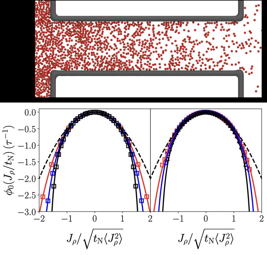
2

theory in the context of nanoscale transport phenomena
                                                                    φE (j)                                           ψE (λ)
with a focus on classical molecular systems. We illus-
trate how fluctuations and their associated nonlinearities                      j
can be treated consistently from a molecular, rather than
                                                                                       E               J
phenomenological, perspective. We first consider basic
formal results, reviewing past work clarifying the struc-
ture of nonequilibrium fluctuations and their connection                                                                       λ
to response functions in principle. We then consider ad-
vances in numerical approaches that allow those formal
results to be brought to bare on complex systems in prac-
                                                               FIG. 1. Illustration of the expected form of the rate function,
tice. We illustrate some specific applications of this view    φE (j), and cumulant generating function, ψE (λ), under small
on transport, where large deviation functions have been        applied field E (solid lines) and at equilibrium (dashed lines).
evaluated in models that provide a realistic description of
physical systems. Finally, we conclude briefly on what is
needed to extend this theory of nonequilibrium steady-
states to more general classes of systems, and discuss         the characteristic function associated with fluctuations of
open areas worthy of pursuit.                                  J can be computed from the Laplace transform of Eq. 2,

                                                                                                  1
                                                                              ψE (λ) = lim            ln e−λJ    E
                                                                                                                              (3)
II.   LARGE DEVIATIONS IN PRINCIPLE                                                        tN →∞ tN

                                                               where ψE (λ) is known as a scaled cumulant generating
   A central problem in nonequilibrium statistical me-
                                                               function, and depends on the Laplace parameter λ but
chanics is the evaluation of the probability distribution
                                                               not tN . Derivatives of ψE (λ) with respect to λ evaluated
of fluctuating variables. Large deviation theory provides
                                                               at λ = 0 yield the time intensive cumulants of J.
a path to do this. In the context of transport and dy-
namical systems, the relevant stochastic variable whose           The pair φE (j) and ψE (λ) are related to partition func-
extent can be take arbitrarily large is a time integrated      tions for path ensembles that are either conditioned to ex-
current, J, or generalized displacement,                       hibit a value of J or that are statistically biased towards
                                                               different J’s through λ.57,58 They completely character-
                          Z    tN                              ize the fluctuations of the current within a nonequilib-
                     J=                 ˙
                                    dt J(t)             (1)    rium steady-state. When both φE (j) and ψE (λ) exist
                           0                                   and are smooth and differentiable, they contain the same
                                                               information. Specifically, they are related to each other
        ˙
where J(t)   is an instantaneous flux at time t, and tN is     through a Legendre-Fenchel transform,1
the observation time, taken to be larger than any char-
                                ˙
acteristic correlation time of J(t).                                                φE (j) = inf [ψE (λ) + λj]                (4)
                                                                                              λ
   The fluctuations of J can be characterized by a prob-
ability distribution, or alternatively by its characteristic   as follows from a saddle point approximation to the in-
function. For a dynamical property or a system away            tegral definition, valid in the long time limit. Further,
from equilibrium where Boltzmann statistics do not hold,       when this relation holds, trajectories taken from the con-
the calculation of either is a daunting task. The funda-       ditioned ensemble are equivalent to trajectories under the
mental principle of large deviation theory is that currents    statistical bias.59 Figure 1 illustrates these two quantities
that are correlated over a finite amount of time admit an      near equilibrium.
asymptotic, time intensive form of the logarithm of their         Many formal results have been derived for large devi-
distribution function2,4                                       ation functions of time integrated currents. Some of the
                          1                                    most foundational and useful in the context of nanoscale
          φE (j) = lim      lnhδ(jtN − J[X])iE          (2)    transport are reviewed below. In the following, a dis-
                   tN →∞ tN
                                                               tinction is drawn between systems near equilibrium and
where φE (j) is known as the rate function and is a natural    those far from it.
variable of the time intensive current, j = J/tN . We will
adopt a notation that distinguishes averages in the pres-
ence of an external field E that drives the current, where     A.   Fluctuations near equilibrium
h..iE denotes an average in the steady state generated by
field E, and δ(jtN − J[X]) is Dirac’s delta function eval-        Assuming that the departure from equilibrium is small
uated using a fluctuating current J[X] that depends on         and that Boltzmann statistics hold, Onsager originally
a trajectory X. This asymptotic form implies that de-          conjectured that the log-probability of a current fluctua-
viations away from the mean are exponentially unlikely,        tion was given by the entropy production to create it.38,39
with a rate set by φE (j). From large deviation theory,        In what he called a dissipation function, now identifiable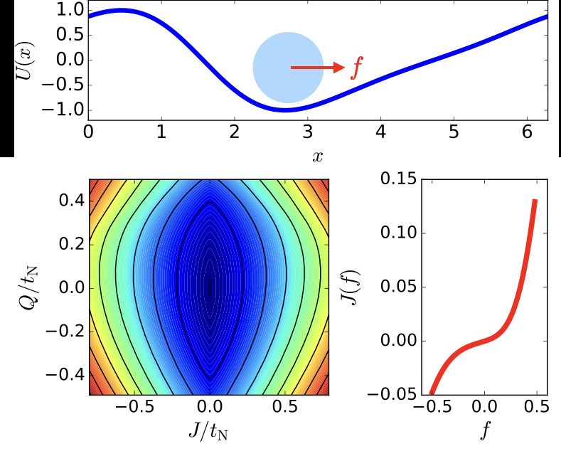
3

as a rate function, the log-probability of a current fluc-     will restrict our discussion to processes describable by a
tuation was given by                                           Langevin equation.66 For concreteness, in the next few
                                                               sections, we will consider an underdamped equation of
                      φ0 (j) ≈ −βEj/4                   (5)    the form
                             = −βj 2 /4χ
                                                                       ṙ = vi , mi v̇i = Fi rN + Ei − γi vi + ηi

                                                                                                                      (9)
where in the second line the dependence on the field has
been eliminated through a phenomenological linear law          for particle i where the final two terms obey a local de-
relating the current to the field, j = χE, through a con-      tailed balance with a temperature Ti , by dissipating en-
stant of proportionality χ that is observed to be a gen-       ergy through the friction, γi , and adding energy by a
eralized conductivity. The Gaussian form for the current       random force ηi (t) with Gaussian statistics described by
fluctuations is consistent with microscopic reversibility in   hηi (t)i = 0, hηi (t)ηjT (t0 )i = 2γi kB Ti 1δij δ(t − t0 ), where
equilibrium that requires φ0 (j) is an even function of j.     kB is Boltzmann’s    constant and 1 is the unit matrix. The
                                                               force, Fi rN , is assumed to be gradient but depends on

   The corresponding scaled cumulant generating func-
tion is,                                                       the full configuration of the system, rN , and Ei is an
                       ψ0 (λ) = λ2 χ/β                  (6)    external field driving a nonequilibrium steady-state. In
                                                               the limit that Ei = 0 and Ti = T for all i, the system
where under the Gaussian approximation to the current          evolving with Eq. 9 will develop a Boltzmann distributed
fluctuations, ψ0 (λ) is quadratic in λ. As a scaled cu-        steady state and exhibit microscopic reversibility.67
mulant generating function, derivatives of ψ0 (λ) with re-        A consequence of the underlying microscopic reversibil-
spect to its argument provide the intensive cumulants of       ity of Eq. 9, and its local detailed balance, is that when
J, for example                                                 driven away from equilibrium its trajectories satisfy the
                                                               Crooks fluctuation theorem.34 In terms of a scalar current
                  d2 ψ0 (λ)            1
                                    =    hδJ 2 i0       (7)    j driven by a scalar field E, this symmetry is manifest in
                    dλ2       λ=0     tN                       the current rate function as
                                    = 2χ/β
                                                                                  φE (j) − φE (−j) = βEj                    (10)
which relates the conductivity with the variance of the
current, χ = βhδJ 2 i0 /2tN . In the long time limit this is   due to Kurchan for diffusive dynamics.33 This symmetry
equivalent to                                                  means that currents that evolve in opposition to their
                        Z tN                                   driving field are exponentially unlikely with a scale set
                χ=β           dt hj(0)j(t)i0            (8)    by the entropy production associated with the current.
                          0                                    This fluctuation theorem is a specific realization of a
assuming current correlations decay faster than 1/t. The       more general fluctuation theorem for the total entropy
first form of the fluctuation dissipation relation is known    production,68 can be generalized to multiple currents,12
as an Einstein-Hefland moment.60,61 Equation 8 follows         and is a microscopic statement of the second law of
from time reversal symmetry, and results in a traditional      thermodynamics.69 Importantly this relationship is valid
Green-Kubo expression for the response of a current in         for arbitrary E. When E = 0, it reduces to a condi-
terms of an integrated time correlation function.62–64         tion that the equilibrium probability of a current is an
   The Gaussian form of φ0 (j) is valid only for small j,      even function, from which the linear response relation-
as is the subsequent linear response relationship that fol-    ships discussed above follow.70 Its equivalent statement
lows. Their utility derives from their thermodynamic ori-      in terms of the scaled cumulant generating function is
gin, in which the entropy production uniquely determines                           ψE (λ) = ψE (βE − λ)                     (11)
the response. This endows linear response relationships
with great generality. They are equally valid indepen-         which in the context of stochastic dynamics is known as
dent of the specific dynamics of the system, provided the      Lebowitz-Spohn symmetry,31 or in the deterministic limit
large deviation form holds. In practice, this requires that    as Gallavati-Cohen symmetry.32 As these symmetry rela-
correlation times for the current are finite.                  tions are thermodynamic in origin, equivalent expressions
                                                               exist independent of the specific evolution equation.
                                                                  Around an equilibrium steady-state, Eq. 10 or Eq. 11,
B.   Fluctuations far from equilibrium                         is sufficient to deduce a linear response relationship in
                                                               the form of the fluctuation-dissipation theorem.71 This
   Unlike fluctuations about an equilibrium steady-state,      reflects the fact that, in this specific case, the fluctua-
fluctuations away from equilibrium are not generically         tions of J in equilibrium encode the response of J to the
determined solely by thermodynamic considerations.65           field E. However, for nonlinear response, or linear re-
Thermodynamics can bound the scale of fluctuations             sponse around a nonequilibrium steady-state, additional
and impose specific symmetries, but their detailed form        functional information is needed. One way to proceed
will depend in general on the specific equations of mo-        elaborated upon by Gaspard12 evaluates the average cur-
tion developing those fluctuations. In the following we        rent hJiE in terms of mixed derivatives of ψE (λ). Using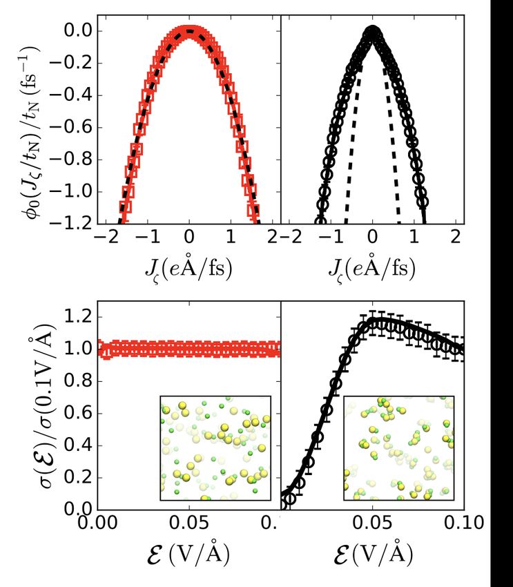
4

the fluctuation theorem, the current up to second order                     φE (j)                                                     q
in the field is                                                                           j                                                  φ̂0 (j, q)

   hJiE   ∂ 2 ψ0 (λ)         βE   ∂ 3 ψE (λ)                (βE)2                             E                  J                                  j
        =                       +
    tN       ∂λ2       λ=0    2   ∂λ2 ∂βE           λ,E=0     2
           hδJ 2 i0       1 dhδJ 2 iE
         =          βE +                                (βE)2   (12)
             2tN         2tN dβE                  E=0
                                                                       FIG. 2. Nonlinear response like current rectification through
where the second line follows from the definition of the
                                                                       a diode can be understood by how (left) current fluctuations
scaled cumulant generating function.12,14 This illustrates             described by φE (j) change at equilibrium (dashed lines) or for
that in addition to knowledge of the fluctuations of J                 large fields (solid lines), or alternatively how (right) current
about equilibrium, it is necessary to know how those fluc-             and activity fluctuations described by φ̂0 (j, q) are correlated
tuations change with an applied field to predict higher                in equilibrium.
order response. This is due to the general breakdown of
the fluctuation-dissipation relationship away from equi-
librium, and the fact that kinetic factors, like the effective
diffusivity hδJ 2 iE , become important within nonequilib-             where ∆DE (q) = DE (q) − D0 (q) is referred to as the
rium steady-states.                                                    excess dynamical activity, the time symmetric analogue
   An alternative way to interpret the fact that equilib-              to the entropy production.
rium fluctuations of J are insufficient to predict the full              While for general dynamical processes and arbitrary
response of a current to a field E is to note that only                currents ∆DE (q) may be complicated, for currents that
near equilibrium are J and E conjugate dynamical quan-                 are linear in the microscopic velocities driven by fields
tities. From Maes and coworkers, away from equilibrium,                that enter linearly into the equation of motion given in
in general the quantity conjugate to E in the path prob-               Eq. 9, ∆DE (q) simplifies significantly. Specifically, we
ability will have components that are asymmetric under                 have found that it can be deduced to be linear in q with
time reversal, as well as components that are symmetric                an additive constant proportional to E 2 .13 This means
under time reversal.72,73 While the fluctuation theorem                that the joint rate function for j and q, driven arbitrarily
uniquely determines the former to be the entropy pro-                  far from equilibrium by E, is related to its equilibrium
duction, the specific form of the latter depends on the                counterpart by
equation of motion. If we denote Q as the fluctuating                     φ̂E (j, q) − φ̂0 (j, q) = βE(j + q)/2 − βχid E 2 /4                   (17)
time reversal symmetric contribution conjugate to E in
the path probability, which is zero on average in equilib-             where χid is the conductivity in the non-interacting par-
rium, then                                                             ticle limit. Analogously, the scaled cumulant generating
                                                                       function is
                             Z    tN
                                                                                           1
                       Q=              dt Q̇(t)                 (13)     ψ̂E (λj , λq ) =    ln e−λj J−λq Q E               (18)
                              0                                                           tN
                                                                                       = ψ̂0 (λj − βE/2, λq − βE/2) − βχid E 2 /4
which is extensive in time with increment Q̇ and q =
Q/tN its intensive counterpart. Considering the joint rate             This implies that, for systems in which Eqs. 17 and 18
function, φ̂E (j, q) for the time intensive j and q, we have           hold, φ̂0 (j, q) acts as a thermodynamic potential that
from the fluctuation theorem                                           completely determines the response of a current to an ap-
                                                                       plied field.13 Further, it implies a nonequilibrium ensem-
               φ̂E (j, q) − φ̂E (−j, q) = βEj                   (14)   ble reweighting principle between steady-states evolved
                                                                       under different applied fields with E and the sum J + Q
while its complement                                                   acting as conjugate dynamical variables.74 While this
                                                                       is restricted to diffusions of the form of Eq. 9, a simi-
             φ̂E (j, q) + φ̂E (−j, q) = βDE (q)                 (15)   lar result has recently been proved for driven exclusion
                                                                       processes.75 Using these relations, the average current
defines a function of q that encodes the time symmetric                hJiE is
contribution, βDE (q), to the joint rate function φ̂E (j, q).                                                            2
                                                                                     hJiE = hJeβE(J+Q)/2−βχid tN E           /4
                                                                                                                                  i0            (19)
This function can be readily calculated from an explicit
equation of motion like that in Eq. 9, and specific forms              valid for arbitrary E. To second order in the field, the
are shown in Sec. III A and Sec. IV C. Using these two                 current is given by
relations, both valid for arbitrary E, we can relate the
                                                                       hJiE   ∂ 2 ψ̂0 (λj , λq )         βE   ∂ 3 ψ̂0 (λj , λq )              (βE)2
joint rate function φ̂E (j, q) under the applied field to its               =                               −
                                                                        tN          ∂λ2j                  2       ∂λ2j ∂λq                      4
value in the absence of the field, φ̂0 (j, q), as                                                  λ=0                                 λ=0
                                                                               hδJ 2 i0 βE   hδJ 2 δQi0 (βE)2
     φ̂E (j, q) − φ̂0 (j, q) = βEj/2 + β∆DE (q)/2               (16)         =             +                                                      (20)
                                                                                 tN      2       tN       4
5
where we have invoked the time reversal symmetry of the be calculated. In Sec. IV A we review a study on the
equilibrium average to eliminate terms that average to 0 diffusive transport of a tagged active Brownian particle,
and employed the fact that hJi0 = hQi0 = 0.13 Compar- which can be solved exactly by integrating out degrees of
ing to Eq. 12, we observe that the correlations between freedom with a many body expansion.82
J and Q, hδJ 2 δQi0 , encode the change of the fluctua- Absent analytical solutions, basis set techniques can
tions in J with the applied field through an equilibrium be used to numerically solve Eq. 21. For example Fig.
expectation value. These two views are illustrated in 3 illustrates the joint rate function φ̂0 (j, q) for diffusive
Fig. 2. Thus, to construct response theories for nanoscale transport in a periodic ratchet potential. An overdamped
transport where nonlinearities and departures from equi- equation of motion reduces the dimensionality of the sys-
librium are commonplace, one can either determine the tem to a simple periodic coordinate, r,
functional dependence of the distribution of currents on
the driving field, or consider the joint distribution of the γ ṙ = F (r) + f + η 0 ≤ r ≤ 2π (23)
current and activity in equilibrium.
and φ̂0 (j, q) is the joint rate function for j = ṙ and cor-
responding dynamical activity q = −γ −1 F (r), the neg-
III. LARGE DEVIATIONS IN PRACTICE ative external force. As a periodic problem, Eq. 21 can
be diagonalized using a Fourier basis and φ̂0 (j, q) evalu-
While large deviation functions have been evaluated in ated using an analogue of Eq. 4. In this specific system,
analytically tractable systems, and in lattice models, the F (r) = −∂r U (r), where U (r) = − sin(r + sin(r)/2), lacks
application of large deviation theory to nanoscale trans- inversion symmetry, and the nonlinear response of j to
port problems with detailed molecular or mesoscopic an applied force f exhibits current rectification, see Fig.
models has been limited. In large part this is due to the 3. The joint j and q fluctuations encode this asymmet-
lack of suitable numerical tools. With recent advances ric response. In the joint rate function, fluctuations that
by us and others, this formalism can now be brought increase q are correlated with increasing the scale of fluc-
to bare on complex systems. Below we review some ex- tuations in j, or hδJ 2 δQi0 > 0, and vice versa, leading to
isting techniques for evaluating large deviation functions a larger current and differential mobility for f > 0 than
numerically. We distinguish two existing approaches that for f < 0, from Eq. 20. For interacting problems, sig-
either attempt to solve for a large deviation function di- nificant developments into compact basis sets employing
rectly by solving a generalized eigenvalue equation from matrix and tensor product states have advanced the state
those that are based on estimating them stochastically of the art for lattice transport problems.83–87 However,
by sampling rare trajectories. these have not yet been translated into the continuum
for molecular problems.
A very attractive alternative to the generalized eigen-
A. Evaluating large deviation functions directly value equation for the direct evaluation of the large de-
viation functions is through variational principles that
The traditional approach to compute the large ψE (λ) satisfies.88–92 While the non-Hermitian nature
deviation functions is to employ the Feynman-Kac of Lλ precludes traditional eigenvalue-based variational
theorem,2,59,76 which relates the scaled cumulant gener- statements from being formulated, a result from optimal
ating function to the largest eigenvalue of a tilted or de- control theory can be used. Specifically, employing an
formed operator.31 For the Markovian auxiliary system with additional drift u(rN , vN )
P process in Eq. 9,
and an observable of the form j = i ai · ṙi + bi · v̇i , the
ψE (λ) = sup [−λhjiu + h∆Uiu ] (24)
generalized eigenvalue equation is u(rN ,vN )
Lλ Rλ = ψE (λ)Rλ (21) where
X u
and ∆U = (u − 2mv̇i + 2Fi + Ei − γi v) (25)
4kB Ti γi
X 1 i
Lλ = vi ∇ri + [Fi (rN ) + Ei ] (∇vi + λbi )
i
mi is the change in the action following from a Girsanov
kB Ti γi 2
transform and application of Jensen’s inequality. Here
+ (∇vi + λbi ) − λai vi (22) h. . . iu denotes an average with the additional drift. The
m2i
maximization is over all control drifts and is solved by
where the adjoint of L0 is the Fokker-Planck operator and the dominant eigenvector with component ui (rN , vN ) =
Rλ is the dominate right eigenvector. Typically the force 2kB Ti /γi ∇i ln Rλ .59,93,94 While the eigenvector is many-
Fi (rN ) complicates the analytic solution of the eigen- bodied, low rank approximate forms have been optimized
value equation. In force-free cases, like free diffusion77 using analogues of variational Monte Carlo90 and ma-
and open Levy walks,78 and linear systems, like collec- chine learning,95,96 which have been found to yield ac-
tions of harmonic oscillators79 and Ornstein-Uhlenbeck curate results. The variational Monte Carlo approach
processes,58,80,81 the cumulant generating function can is made efficient by explicit forms for the derivatives6
the dynamics that generate Pλ [X] are determined by the
solution of the generalized eigenvalue problem in Eq. 21.
Therefore, the weight factor exp[−λJ] is typically incor-
porated through an importance sampling process on top
of direct dynamical propagation.
Two main classes of trajectory importance sampling
exist, transition path sampling99 and diffusion Monte
Carlo, or the cloning algorithm.5–7 Transition path sam-
pling performs a sequential update to a single trajec-
tory with fixed time in the manner of a Markov chain
Monte Carlo algorithm, though through the trajectory
space.100 The weighting factor is accommodated by a
trajectory acceptance criteria. The application of tran-
sition path sampling to large deviation functions was
first applied in the context of equilibrium glass formation
problems,48,101 and later extended to transport prob-
lems evolving non-detailed balanced dynamics.8,41 Alter-
natively, the cloning algorithm propagates an ensemble of
FIG. 3. (top) Illustration of a Brownian particle in a ratchet short trajectories in parallel using the reference dynam-
potential subject to an applied force. (Bottom left) The joint ics. Each trajectory accumulates a local weight which is
rate function φ̂0 (j, q) encoding the response of the particle’s used as a basis for a population dynamics that reduce the
current. (Bottom right) The associated current as a func- variance of the weights by a branching and annihilation
tion of the applied drift force computable from φ̂0 (j, q) using process. The cloning algorithm has been used widely in
Eq. 19. model transport problems.42–46
Both transition path sampling and the cloning algo-
rithm can evaluate large deviation functions sufficiently
of Eq. 24 with respect to the added drift.90 Further, accurately to be used to compute transport coefficients.
perturbative corrections in the form of a cumulant ex- In particular, in recent work, we showed that the use of
pansion can be formulated to increase the accuracy of the cloning algorithm can yield statistically superior es-
the estimate at the cost of breaking the variational timates of linear transport coefficients using the direct
structure.90,97 This method has been applied to low calculation of the curvature of the large deviation func-
dimensional models and colloidal assemblies in shear tion through Eq. 7, as compared to their direct evaluation
flows.98 With the concurrent development of expressive through Green-Kubo theory.102 This was demonstrated
forms for u(rN , vN ), this technique is poised to be widely in the calculation of the thermal conductivity in a WCA
applied to molecular systems. solid and the liquid-solid friction in a Lennard Jones so-
lution. In Sec. IV B we show how this procedure was
used to study the anomalous heat transport in low di-
B. Estimating large deviation functions stochastically mensional carbon lattices.103 The cloning algorithm has
also been used to evaluate the joint large deviation func-
tion of the current and activity, and efficiently estimate
An alternative to the direct evaluation of a large de-
nonlinear response functions by Eqs. 18 and 20. For
viation function is to estimate it by sampling molecular
example, we have analyzed the rectification of heat cur-
dynamics simulations. This direction has seen signifi-
rents in chains of nonlinear oscillators with inhomoge-
cant recent development as a means of avoiding nonequi-
neous mass distributions.13
librium simulations that induce long range correlations
or to evaluate field-dependent differential transport co- While the calculation of linear transport properties
efficients directly. In order to accurately estimate the are tractable even for models with complex forcefields,
large deviation function, one must sample a path ensem- the evaluation of nonlinear response is significantly more
ble that incorporates the exponentially rare fluctuations computationally challenging. This is because the cloning
in the dynamical observable of interest. If PE [X] denotes algorithm, as well as transition path sampling, both aug-
a reference path ensemble driven by a field E, then the ment the propagation of the bare system dynamics with
path ensemble to be sampled to compute ψE (λ) or φE (j) importance sampling, without any guidance from the rare
for a current J is events that contribute to the large deviation function. As
a consequence, for exponentially rarer fluctuations, both
Pλ [X] = PE [X]e−λJ[X]−ψ(λ)tN (26) Monte Carlo algorithms require exponentially more sam-
ples of the targeted stationary distribution as the overlap
where the new path ensemble Pλ [X] is biased by the fac- between it and the proposed distribution becomes expo-
tor exp[−λJ] and normalized by ψ(λ). While the dy- nentially small.8,9,104 Recent advances that incorporate
namics that generates PE [X] are defined by the model, auxiliary dynamics to guide the path sampling using ap-7
proximate solutions to Eq. 24 have been successful at A. Active brownian particle diffusion
significantly dropping the computational cost of both al-
gorithms. In Ref. 90 we report a gain of over 3 orders Much of the framework outlined above is agnostic to
of magnitude in the statistical efficiency of the cloning whether the system is evolving within an equilibrium or
algorithm with a guiding force. Various approaches nonequilibrium steady-state. As an illustration of the
have incorporated analytical approximations,9,56 vari- latter, the diffusion of a tagged particle in an active fluid
ationally optimized ansatzes,90,91 or feedback control is considered.82 An active fluid is one in which a constant
procedures.105–107 source of energy is continuously converted into directed
An alternative route we have pursued for the evalua- motion of individual particles, and can be realized with
tion of nonlinear current-field relationships is to leverage synthetic colloids or swimming bacteria.112–121 In such a
the reweighting principle valid between equilibrium and fluid, novel transport processes disallowed in equilibrium
nonequilibrium ensembles when Eq. 17 holds. In such a can occur due to the time-reversal symmetry breaking in-
case, the probability of observing a trajectory in a driven herited from the persistent dissipation.122–125 For exam-
ensemble is equal to the probability of that trajectory in ple, the viscosity of the fluid can acquire odd components,
equilibrium times a weighting factor and the Stokes-Einstein relation can break down.126–128
The specific active fluid previously considered was a
2
collection of active Brownian particles in two-dimensions.
P0 [X] = PE [X]e−β(J+Q)E/2+βχid E /4
(27) In addition to interparticle interactions and random bath
forces, active Brownian particles are convected along a
velocity vector that rotates diffusively with constant am-
where the sum J + Q depends on the trajectory, but plitude vo . The specific equations of motion are of the
βχid E 2 /4 is a trajectory independent constant. Using a form of Eq. 9 in an overdamped limit,
series of different nonequilibrium ensembles at different
values of E, rare equilibrium fluctuations of the current s
and activity can be probed.74,108 Employing standard 1 N 2kB T p
ṙi = Fi r +vo ei + ηi , θ̇i = 2Dθ ξi (28)
equilibrium techniques like the weighted histogram anal- γ γ
ysis method109 or multistate Bennet acceptance ratio,110
many simulations can be combined to enhance expec- where ei = {cos(θi ), sin(θi )} is the unit vector which
tation values at each field. Analogous to standard his- undergoes diffusive motion due to the random force
togram reweighting methods used between equilibrium ξi and rotational diffusion constant Dθ . The inter-
particle force Fi rN was derived from the gradient of
ensembles,111 this approach offers an attractive ability
to compute the average current as a continuous function a WCA potential.129 To characterize diffusive transport,
of the field using Eq. 19. Formally, this bypasses assump- the statistics of single particle displacements was consid-
tions of the existence of a Taylor series expansion of the ered,
current in terms of the applied field. Practically, it avoids Z tN
having to numerically evaluate the gradient as would be
Jρ (tN ) = dt ṙi (t) (29)
necessary in direct nonequilibrium simulations. In Sec. 0
IV C we illustrate how this procedure is used to study the
field dependence of the ionic conductivity in electrolyte in the long time limit, tN → ∞. The distribution of par-
solutions. ticle displacements was derived by solving the equivalent
eigenvalue equation in Eq. 21 for a tagged active Brown-
ian particle. This was possible in an interacting system
because Eq. 21 took the form of a Matheiu equation,130
with a single unknown λ-dependent parameter resulting
IV. APPLICATIONS from the closure of a BBGKY-like hierarchy.131 This pa-
rameter could be computed numerically from an integral
over an empirical pair distribution function.
Building upon the formal developments connecting As reported in Ref. 82, distribution of single particle
large deviation theory and nanoscale transport, and the displacements was found to be non-Gaussian, except in
recent advances in numerical techniques to characterize the limit of passive particles. Example rate functions,
dynamical fluctuations in complex systems, a number of φ0 (Jρ /tN ), are shown in Fig. 4, which while parabolic
different canonical transport problems have bene studied. around their means exhibited short tails reflective of sup-
In the following, we illustrate a few specific examples in pressed fluctuations around large conditioned displace-
which the currents result from single tagged particles or ments. From the variance of the distribution computed
their collections. We consider the examples of the trans- at fixed density ρ, the self-diffusion coefficient could be
port of mass, energy and charge. In each, large deviation determined,
theory enables the computational study of either linear
or nonlinear phenomena, in a way not feasible without 1
D(ρ) = lim hJ 2 i (30)
the tools it provides. tN →∞ 2tN ρ8
agreement with those computed from the rate function.
Nonlinear corrections, while relevant for the observed
motility induced phase separation in these materials,133
remain to be tested numerically.
B. Heat transport in low dimensional solids
Utilizing our observations that the statistical con-
vergence of linear transport coefficients is accelerated
when evaluated from the large deviation function rela-
tive to traditional Green-Kubo expressions,102 this ap-
proach was applied to study the thermal conduction
through low dimensional carbon lattices.103 Heat trans-
port within carbon nanotubes and graphene sheets have
received considerable recent attention, due to experi-
mental and simulation reports claiming a violation of
Fourier’s law of conduction.18–21 These reports expand
on a large literature of anomalous transport in systems
that can be taken macroscopically large in fewer than
three-dimensions.134–137 Experimentally, reports on low
FIG. 4. The response of a system of active Brownian particles dimensional lattices have shown indications of anoma-
to a density gradient (top) is computable from the rate func- lous conductivities, though difficulties extracting defini-
tion of single particle displacement statistics (bottom) for a tive values are complicated by boundary effects.
variety of self-propulsion velocities (left) and densities (right). To understand the mechanism of heat transport in low
The symbols denote numerical calculations from the cloning
dimensional carbon lattices, the energy current fluctua-
algorithm, solid lines the exact solution of the generalized
eigenvalue equation, and the dashed lines a Gaussian rate
tions were considered within a nanotube and a graphene
function with unit variance. Figure adapted from Ref. 82. sheet. The individual atoms evolved deterministically in
the bulk of the material through the solution of New-
ton’s equation of motion, but two stochastic reservoirs
at each end imposed a constant temperature through the
which was in excellent agreement with direct estimates Langevin equation in Eq. 9. The geometry is illustrated
from the mean-squared displacement over a range of self- in Fig. 5. The atoms interacted through the conserva-
propulsion velocities and densities. Generically, the self- tive force described by the gradient of a Tersoff potential
diffusion coefficient decreased modestly with increasing parameterized to recover the phonon spectrum of carbon
density, and increased significantly with increasing self- nanostructures.138
propulsion. The heat transport was studied by monitoring the en-
The tagged particle current fluctuations encoded by ergy exchanged with the stochastic reservoirs. Specif-
the large deviation rate function provided the response ically, the energy current through the kth reservoir is
of a hydrodynamic current, jρ , generated from a slowly given by a sum over Nk atoms in that region,
varying spatial density, ρ(r). This is analogous to Nk
X
the perspective in Eq. 12. From the Kramers-Moyal jk (t) = [mv̇i (t) − Fi (t)] · vi (t) (32)
expansion,132 jρ can be expressed as a gradient expansion i∈k
∞ and thus the energy exchanged from the rth reservoir into
X (−1)n n−1 n
jρ = − ∂ M [ρ(r)]ρ(r) (31) the lth reservoir over a time tN is the integrated current
n=1
n!tN r Z tN
J = dt [jl (t) − jr (t)] (33)
where M n [ρ(r)] is the local density-dependent nth cen- 0
tered moment of the current, h(Jρ −hJρ i)n i. To first order in the long time limit, tN → ∞. If the system is main-
at low density, the mass current is linear in the density tained at thermal equilibrium, with the reservoirs fixed
gradient and is given by Fick’s law, jρ ≈ −D(ρ)(∂ρ/∂r), to a common temperature T and separated by a distance
where D(ρ) is the proportionality constant relating the L, the conductivity is computable from the mean-squared
current to the gradient. Thus, mass transport is Fickian fluctuations of the energy exchanged with the reservoirs,
in that the diffusion constant determines the response
of a small density gradient, but nonlinear responses are hJ i∆T
κL = lim lim − L
computable from the density dependence of the current ∆T →0 tN →∞ tN ∆T
distribution. Direct estimates of gradient diffusivity from hJ2 i0
the simulation of an initial density gradient were in good = lim L (34)
tN →∞ 2tN kB T 29
is better described by a Lévy walk rather than sim-
ple diffusion.135,139–141 However, recent results suggests
these anomalous scalings might plateau at even larger
lengths than considered in our study.142 While this cal-
culation considered linear phenomena, generalizations to
heat current rectification have been considered in model
systems.13
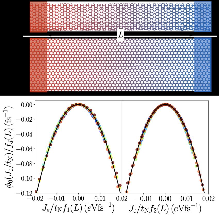
C. Ionic conductivity at high fields
The framework presented here allows arbitrary non-
linear transport behavior to be considered on the same
footing as traditional linear response. To explore the
former, our approach was applied to nonlinear electroki-
netic phenomena in ionic solutions. Advances in the
fabrication and observation of nanofluidic devices have
enabled the study of electrokinetic phenomena on the
smallest scales15,17,143 . When confined to nanometer di-
mensions, large thermodynamic gradients can be gener-
ated, driving nonlinear responses such as field dependent
transport coefficients and nonequilibrium behaviors like
FIG. 5. Large deviation scaling of the heat current for a current rectification144–146 . Existing theories for nonlin-
nanotube (d = 1) and graphene sheet (d = 2). (Top) Illus-
ear conductivities are valid only in the dilute solution
trates the two geometries in contact with stochastic reservoirs.
(Bottom) Rate functions for the heat current for a variety of regime.147–149
system sizes, collapsed bypscaling functions that asymptot- The field dependence of the ionic conductivity was
ically approach f1 (L) ∼ L/` and f2 (L) ∼ L ln L/` with studied in strong and weak electrolytes,74 developing a
characteristic length `. This figure is adapted from Ref. 103. contemporary perspective on the so-called Onsager-Wien
effect.150 Initially a monovalent salt was studied in im-
plicit solvents with dielectric constants of 10 and 60 to
model a weak and strong electrolyte, respectively. The
where at long times, for a finite open system, the mean- ions evolved with Eq. 9, with frictions chosen to recover
squared fluctuations are expected to scale linearly with the self diffusion coefficients in the dilute limit. In or-
time. This exact expression follows from the definition of der to predict the field dependent ionic conductivity from
κL as the differential increase of the average heat current equilibrium fluctuations, knowledge of both the ionic cur-
with a temperature difference and the stochastic process rent
in Eq. 9. This specific form is an example of an Einstein- X Z tN
Helfand moment, equivalent to a Green-Kubo relation.61 Jζ = dt zi vi (35)
To compute the rate function of heat current fluctua- i 0
tions, the Monte Carlo procedure discussed in Sec. III B
was employed to importance sample the probability of where zi is the charge on ion i, and its time reversal
an integrated current at equilibrium. Using a range of symmetric counter part, and the dynamical activity,
λ’s, a set of φλ (J ) was related to φ0 (J ) using histogram tN
reweighting,109 enabling the construction of φ0 (J ) far
XZ zi
mi v̇i − Fi rN
Qζ = dt (36)
into the tails of the distribution. These are shown in i 0 γi
Fig. 5 for both carbon nanotubes and graphene sheets.
Studying a range of system lengths, φ0 (J ) was found to which is a difference between momentum flux and inter-
be collapsed with a dimensional-dependent scaling func- molecular force weighted by the charge and friction is
tion fd (L), from which the system-size-dependence of needed. Using nonequilibrium ensemble reweighting, the
the conductivity was deduced, κL ∝ fd (L)/L. For car- joint rate function φ0 (Jζ , Qζ ) was computed far into its
bon nanotubes, the thermal conductivity κL was found tails. This reweighting procedure is made possible by
to increase as the square root of the length of the nan- the relationship given in Eq. 17, where typical fluctua-
otube, while for graphene sheets the thermal conductivity tions of Jζ and Qζ for simulations under finite applied
was found to increase as the logarithm of the length of fields can be used to reconstruct rare fluctuations in the
the sheet. The particular length dependence and non- absence of a field. The marginalization of the joint distri-
linear temperature profiles place carbon lattices into a bution constructed from a series of nonequilibrium sim-
universality class with nonlinear lattice models, and sug- ulations onto the current is shown in Fig. 6. For the
gest that heat transport through carbon nanostructures strong electrolyte, the current fluctuations were found to10
sian current statistics, the strong electrolyte exhibits
a field-independent conductivity equal to its Nernst-
Einstein value. By contrast, the weak electrolyte, with
its marked non-Gaussian current statistics, exhibits a
strongly field dependent conductivity. For the weak elec-
trolyte, an initially low value of σ(E) increases, exhibits a
small maximum, before plateauing to its Nernst-Einstein
limit. The maximum reflects the increased fluctuations at
fields just strong enough to dissociate ion pairs. Oppos-
ing these enhanced current fluctuations are negative cor-
relations between j and q, which reflect ionic relaxation
dynamics whereby electric fields generated by distortions
of the ionic cloud around an ion are anti-correlated with
displacements of the ion in the direction of the exter-
nal field. Extensions of this analysis to explicit solvent
models has been recently undertaken,108 and their im-
plications for simulations with explicit nanoconfinement
remains to be studied.151–153
V. BEYOND
The perspective articulated here illustrates how to
leverage formal advances in nonequilibrium statistical
mechanics and novel numerical techniques to address
FIG. 6. Ionic current fluctuations (top) and associated field
dependent conductivities (bottom) of a strong (left) and weak
contemporary problems in nanoscale transport. While
(right) electrolyte solution. Insets illustrate characteristic significant strides have been made recently in applying
snapshots of the weak and strong electrolyte. Figure adapted large deviation theory to molecular systems driven far
from Ref. 74. from equilibrium, there are clearly outstanding questions.
First, there are technical issues associated with the ap-
propriate equation of motion to describe molecular sys-
tems away from equilibrium. Near equilibrium, ensemble
be incredibly Gaussian. For the weak electrolyte, locally equivalence154 requires linear response functions to be
Gaussian fluctuations around its mean broaden signifi- equal whether they are propagated under Newtonian or
cantly into fat tails. The tails were well described by stochastic equations of motion, provided the character-
a second Gaussian with larger variance, manifesting the istic timescale of the bath is large. Away from equilib-
suppression of current fluctuations when ions are paired rium, however, nonlinear response functions depend on
in the weak electrolyte and its enhancement when they the details of the equation of motion. The constant sup-
dissociate upon conditioning on a large current. ply of energy through an applied field requires a means
With the joint rate function, the differential conduc- to dissipate that energy in order to evolve a nonequilib-
tivity, σ(E), was computed as a continuous function of an rium steady state, so absent explicit boundaries a ther-
applied field E. This follows from the definition of σ(E), mostat of some sort must be used. While in some cases
as the differential change in the the current density with the details of the thermostat can be motivated physi-
applied field cally, extending the nonlinear response formalism and
1 dhJζ iE sampling algorithms discussed here to non-Markovian
σ(E) = (37) and deterministic equations of motion would provide
tN V dE
1 for alternative modeling choices and further general-
= h(δJζ2 + δJζ δQζ )eβ(Jζ +Qζ )E/2 i0 ity. Typically physically derived non-Markovian equa-
2tN kB T V tions can be embedded to yield Markovian models in
where V is the system volume and the long time limit, larger phase spaces.155,156 Exploring connections to other
tN → ∞ is taken to evolve a nonequilibrium steady-state. response formalisms employed with deterministic ther-
While the first line is a definition, the second line employs mostats would undoubtedly be fruitful.157–159 Similarly,
the nonequilibrium ensemble reweighting relation. we have focused entirely on classical systems, but ex-
Figure 6 illustrates the differential conductivity com- tending this perspective to quantum mechanical trans-
puted in this way, which is in good agreement with that port problems would undoubtedly yield novel insights.
evaluated from a numerical derivative of the current- In weak coupling regimes this is likely possible; however,
field relationship; however, the latter is statistically much away from these regimes it is uncertain.160,161
more difficult to converge. As anticipated from the Gaus- Second, there are issues of how to translate con-11
nections between underlying microscopic dynamics and 8 U. Ray, G. K.-L. Chan, and D. T. Limmer, “Importance sam-
mesoscopic behavior into novel design principles. The pling large deviations in nonequilibrium steady states. i,” The
response theories relate particular dynamical correla- Journal of chemical physics 148, 124120 (2018).
9 U. Ray, G. K.-L. Chan, and D. T. Limmer, “Exact fluctuations
tions to emergent transport phenomena, and have been of nonequilibrium steady states from approximate auxiliary dy-
successfully used to explain experimental observations. namics,” Physical review letters 120, 210602 (2018).
10 G. Gallavotti, “Extension of onsager’s reciprocity to large fields
However, inverting that relationship, and rationally de-
signing a molecular system with a target emergent re- and the chaotic hypothesis,” Physical Review Letters 77, 4334
(1996).
sponse is difficult. A potential route to this inverse de- 11 H. Shibata, “Green–kubo formula derived from large deviation
sign is to view Eq. 24 as a cost function to be optimized. statistics,” Physica A: Statistical Mechanics and its Applications
Its interpretation is clear, with the added drift being the 309, 268–274 (2002).
12 P. Gaspard, “Multivariate fluctuation relations for currents,”
smallest change to an equilibrium system to make a spe-
cific current response typical within its steady state. In- New Journal of Physics 15, 115014 (2013).
13 C. Y. Gao and D. T. Limmer, “Nonlinear transport coefficients
deed, this insight has already been used in the context from large deviation functions,” The Journal of chemical physics
of nonequilibrium self-assembly,98 and in the design of 151, 014101 (2019).
flow fields for tracer particles.162 A number of outstand- 14 M. Barbier and P. Gaspard, “Microreversibility, nonequilibrium
ing challenges in renewable energy, separations, and com- current fluctuations, and response theory,” Journal of Physics
putation could be solved provided a nonequilibrium in- A: Mathematical and Theoretical 51, 355001 (2018).
15 S. Faucher, N. Aluru, M. Z. Bazant, D. Blankschtein, A. H.
verse design principle.163 Within the perspective here, Brozena, J. Cumings, J. Pedro de Souza, M. Elimelech, R. Ep-
this seems possible. sztein, J. T. Fourkas, A. G. Rajan, H. J. Kulik, A. Levy,
A. Majumdar, C. Martin, M. McEldrew, R. P. Misra, A. Noy,
T. A. Pham, M. Reed, E. Schwegler, Z. Siwy, Y. Wang, and
M. Strano, “Critical knowledge gaps in mass transport through
VI. ACKNOWLEDGMENTS single-digit nanopores: A review and perspective,” The Journal
of Physical Chemistry C 123, 21309–21326 (2019).
16 T. Mouterde, A. Keerthi, A. R. Poggioli, S. A. Dar, A. Siria,
The authors would like to thank Garnet Chan, Avishek
A. K. Geim, L. Bocquet, and B. Radha, “Molecular streaming
Das, Juan Garrahan, Phillip Geissler, Trevor GrandPre, and its voltage control in ångström-scale channels,” Nature 567,
Robert Jack, Kranthi Mandadapu, Benjamin Rotenberg 87–90 (2019).
17 Y. Yang, P. Dementyev, N. Biere, D. Emmrich, P. Stohmann,
and Hugo Touchette for useful discussions. This mate-
rial is based upon work supported by NSF Grant CHE- R. Korzetz, X. Zhang, A. Beyer, S. Koch, D. Anselmetti,
and A. Gölzhäuser, “Rapid water permeation through carbon
1954580.
nanomembranes with sub-nanometer channels,” ACS Nano 12,
4695–4701 (2018).
18 C.-W. Chang, D. Okawa, H. Garcia, A. Majumdar, and
VII. AUTHOR CONTRIBUTION STATEMENT A. Zettl, “Breakdown of fourier’s law in nanotube thermal con-
ductors,” Physical review letters 101, 075903 (2008).
19 X. Xu, L. F. Pereira, Y. Wang, J. Wu, K. Zhang, X. Zhao,
D. T. L, C. Y. G and A. R. P wrote the manuscript, S. Bae, C. T. Bui, R. Xie, J. T. Thong, et al., “Length-dependent
designed and performed the research. thermal conductivity in suspended single-layer graphene,” Na-
ture communications 5, 3689 (2014).
20 N. Yang, G. Zhang, and B. Li, “Violation of fourier’s law and
anomalous heat diffusion in silicon nanowires,” Nano Today 5,
VIII. REFERENCES 85–90 (2010).
21 M. Wang, N. Yang, and Z.-Y. Guo, “Non-fourier heat conduc-
tions in nanomaterials,” Journal of Applied Physics 110, 064310
1 H.
(2011).
Touchette, “The large deviation approach to statistical me- 22 A. Siria, M.-L. Bocquet, and L. Bocquet, “New avenues for the
chanics,” Physics Reports 478, 1–69 (2009). large-scale harvesting of blue energy,” Nature Reviews Chem-
2 H. Touchette, “Introduction to dynamical large deviations of
istry 1, 0091 (2017).
markov processes,” Physica A: Statistical Mechanics and its Ap- 23 G. Laucirica, M. E. Toimil-Molares, C. Trautmann,
plications 504, 5–19 (2018). W. Marmisollé, and O. Azzaroni, “Polyaniline for improved
3 L. Bertini, A. De Sole, D. Gabrielli, G. Jona-Lasinio, and blue energy harvesting: Highly rectifying nanofluidic diodes
C. Landim, “Macroscopic fluctuation theory,” Reviews of Mod- operating in hypersaline conditions via one-step functionaliza-
ern Physics 87, 593 (2015). tion,” ACS Applied Materials & Interfaces 12, 28148–28157
4 B. Derrida, “Non-equilibrium steady states: fluctuations and
(2020).
large deviations of the density and of the current,” Journal of 24 M. Lokesh, S. K. Youn, and H. G. Park, “Osmotic trans-
Statistical Mechanics: Theory and Experiment 2007, P07023 port across surface functionalized carbon nanotube membrane,”
(2007). Nano Letters 18, 6679–6685 (2018).
5 C. Giardina, J. Kurchan, and L. Peliti, “Direct evaluation of
25 Z. Zhang, X.-Y. Kong, K. Xiao, Q. Liu, G. Xie, P. Li, J. Ma,
large-deviation functions,” Physical review letters 96, 120603 Y. Tian, L. Wen, and L. Jiang, “Engineered asymmetric het-
(2006). erogeneous membrane: A concentration-gradient-driven energy
6 C. Giardina, J. Kurchan, V. Lecomte, and J. Tailleur, “Simu-
harvesting device,” Journal of the American Chemical Society
lating rare events in dynamical processes,” Journal of statistical 137, 14765–14772 (2015).
physics 145, 787–811 (2011). 26 X. Du and X. Xie, “Non-equilibrium diffusion controlled ion-
7 M. Tchernookov and A. R. Dinner, “A list-based algorithm for
selective optical sensor for blood potassium determination,”
evaluation of large deviation functions,” Journal of Statistical ACS sensors 2, 1410–1414 (2017).
Mechanics: Theory and Experiment 2010, P02006 (2010).12 27 C. Wen, S. Zeng, K. Arstila, T. Sajavaara, Y. Zhu, Z. Zhang, 50 D. T. Limmer and D. Chandler, “Theory of amorphous ices,” and S.-L. Zhang, “Generalized noise study of solid-state Proceedings of the National Academy of Sciences 111, 9413– nanopores at low frequencies,” ACS sensors 2, 300–307 (2017). 9418 (2014). 28 Y. Gao, B. Zhao, J. J. Vlassak, and C. Schick, “Nanocalorime- 51 T. Speck, A. Malins, and C. P. Royall, “First-order phase tran- try: Door opened for in situ material characterization under sition in a model glass former: Coupling of local structure and extreme non-equilibrium conditions,” Progress in Materials Sci- dynamics,” Physical review letters 109, 195703 (2012). ence 104, 53–137 (2019). 52 E. Pitard, V. Lecomte, and F. Van Wijland, “Dynamic transi- 29 N. Freitas, J.-C. Delvenne, and M. Esposito, “Stochastic ther- tion in an atomic glass former: A molecular-dynamics evidence,” modynamics of non-linear electronic circuits: A realistic frame- EPL (Europhysics Letters) 96, 56002 (2011). work for thermodynamics of computation,” arXiv:2008.10578 53 Y.-E. Keta, É. Fodor, F. van Wijland, M. E. Cates, and R. L. (2020). Jack, “Collective motion in large deviations of active particles,” 30 C. Y. Gao and D. T. Limmer, “Principles of low dissipation Physical Review E 103, 022603 (2021). computing from a stochastic circuit model,” arXiv:2102.13067 54 T. Nemoto, É. Fodor, M. E. Cates, R. L. Jack, and J. Tailleur, (2021). “Optimizing active work: Dynamical phase transitions, col- 31 J. L. Lebowitz and H. Spohn, “A gallavotti–cohen-type symme- lective motion, and jamming,” Physical Review E 99, 022605 try in the large deviation functional for stochastic dynamics,” (2019). Journal of Statistical Physics 95, 333–365 (1999). 55 É. Fodor, T. Nemoto, and S. Vaikuntanathan, “Dissipation con- 32 G. Gallavotti and E. G. D. Cohen, “Dynamical ensembles in trols transport and phase transitions in active fluids: mobility, nonequilibrium statistical mechanics,” Physical review letters diffusion and biased ensembles,” New Journal of Physics 22, 74, 2694 (1995). 013052 (2020). 33 J. Kurchan, “Fluctuation theorem for stochastic dynamics,” 56 T. GrandPre, K. Klymko, K. K. Mandadapu, and D. T. Lim- Journal of Physics A: Mathematical and General 31, 3719 mer, “Entropy production fluctuations encode collective behav- (1998). ior in active matter,” Physical Review E 103, 012613 (2021). 34 G. E. Crooks, “Entropy production fluctuation theorem and the 57 D. Chandler and J. P. Garrahan, “Dynamics on the way to form- nonequilibrium work relation for free energy differences,” Phys- ing glass: Bubbles in space-time,” Annual review of physical ical Review E 60, 2721 (1999). chemistry 61, 191–217 (2010). 35 C. Maes, “The fluctuation theorem as a gibbs property,” Journal 58 R. L. Jack, “Ergodicity and large deviations in physical systems of statistical physics 95, 367–392 (1999). with stochastic dynamics,” The European Physical Journal B 36 A. C. Barato and U. Seifert, “Thermodynamic uncertainty re- 93, 1–22 (2020). lation for biomolecular processes,” Physical review letters 114, 59 R. Chetrite and H. Touchette, “Nonequilibrium microcanonical 158101 (2015). and canonical ensembles and their equivalence,” Physical review 37 T. R. Gingrich, J. M. Horowitz, N. Perunov, and J. L. Eng- letters 111, 120601 (2013). land, “Dissipation bounds all steady-state current fluctuations,” 60 E. Helfand, “Transport coefficients from dissipation in a canon- Physical review letters 116, 120601 (2016). ical ensemble,” Physical Review 119, 1 (1960). 38 L. Onsager, “Reciprocal relations in irreversible processes. i.” 61 S. Viscardy, J. Servantie, and P. Gaspard, “Transport and Physical review 37, 405 (1931). helfand moments in the lennard-jones fluid. i. shear viscosity,” 39 L. Onsager, “Reciprocal relations in irreversible processes. ii.” The Journal of chemical physics 126, 184512 (2007). Physical review 38, 2265 (1931). 62 M. S. Green, “Brownian motion in a gas of noninteracting 40 T. Speck, “Thermodynamic formalism and linear response the- molecules,” The Journal of Chemical Physics 19, 1036–1046 ory for nonequilibrium steady states,” Physical Review E 94, (1951). 022131 (2016). 63 M. S. Green, “Markoff random processes and the statistical me- 41 R. L. Jack, I. R. Thompson, and P. Sollich, “Hyperuniformity chanics of time-dependent phenomena. ii. irreversible processes and phase separation in biased ensembles of trajectories for dif- in fluids,” The Journal of Chemical Physics 22, 398–413 (1954). fusive systems,” Physical review letters 114, 060601 (2015). 64 R. Zwanzig, “Time-correlation functions and transport coef- 42 P. I. Hurtado and P. L. Garrido, “Test of the additivity principle ficients in statistical mechanics,” Annual Review of Physical for current fluctuations in a model of heat conduction,” Physical Chemistry 16, 67–102 (1965). review letters 102, 250601 (2009). 65 C. Maes, Non-dissipative effects in nonequilibrium systems 43 C. P. Espigares, P. L. Garrido, and P. I. Hurtado, “Dynamical (Springer, 2018). phase transition for current statistics in a simple driven diffusive 66 R. Zwanzig, Nonequilibrium statistical mechanics (Oxford Uni- system,” Physical Review E 87, 032115 (2013). versity Press, 2001). 44 M. Gorissen, J. Hooyberghs, and C. Vanderzande, “Density- 67 G. E. Crooks, “On thermodynamic and microscopic reversibil- matrix renormalization-group study of current and activity fluc- ity,” Journal of Statistical Mechanics: Theory and Experiment tuations near nonequilibrium phase transitions,” Physical Re- 2011, P07008 (2011). view E 79, 020101 (2009). 68 U. Seifert, “Entropy production along a stochastic trajectory 45 P. I. Hurtado and P. L. Garrido, “Spontaneous symmetry break- and an integral fluctuation theorem,” Physical review letters ing at the fluctuating level,” Physical review letters 107, 180601 95, 040602 (2005). (2011). 69 U. Seifert, “Stochastic thermodynamics, fluctuation theorems 46 F. Turci and E. Pitard, “Large deviations and heterogeneities and molecular machines,” Reports on progress in physics 75, in a driven kinetically constrained model,” EPL (Europhysics 126001 (2012). Letters) 94, 10003 (2011). 70 D. J. Searles and D. J. Evans, “The fluctuation theorem and 47 T. Speck and J. P. Garrahan, “Space-time phase transitions in green–kubo relations,” The Journal of Chemical Physics 112, driven kinetically constrained lattice models,” The European 9727–9735 (2000). Physical Journal B 79, 1–6 (2011). 71 D. Chandler, “Introduction to modern statistical,” Mechanics. 48 L. O. Hedges, R. L. Jack, J. P. Garrahan, and D. Chandler, Oxford University Press, Oxford, UK 40 (1987). “Dynamic order-disorder in atomistic models of structural glass 72 M. Baiesi and C. Maes, “An update on the nonequilibrium linear formers,” Science 323, 1309–1313 (2009). response,” New Journal of Physics 15, 013004 (2013). 49 T. Speck and D. Chandler, “Constrained dynamics of local- 73 M. Baiesi, E. Boksenbojm, C. Maes, and B. Wynants, “Nonequi- ized excitations causes a non-equilibrium phase transition in librium linear response for markov dynamics, ii: Inertial dynam- an atomistic model of glass formers,” The Journal of chemical ics,” Journal of statistical physics 139, 492–505 (2010). physics 136, 184509 (2012).
You can also read