A method for planning the trajectory of a mobile robot in an unknown environment with obstacles
←
→
Page content transcription
If your browser does not render page correctly, please read the page content below
E3S Web of Conferences 270, 01035 (2021)                                 https://doi.org/10.1051/e3sconf/202127001035
WFCES 2021

       A method for planning the trajectory of a mobile
       robot in an unknown environment with obstacles
       Fariza Tebueva1, Andrey Pavlov1,* and Dina Satybaltina2
       1North   Caucasus Federal University, Stavropol 355000, Russia
       2L.N.   Gumilyov Eurasian National University, Nur-Sultan 010000, Kazakhstan

                     Abstract. The known algorithms for planning the trajectory of movement
                     of mobile robots in an unknown environment have high computational
                     complexity or do not allow finding the trajectory that is optimal along the
                     length of the path, while maintaining a safe distance from obstacles. The aim
                     of the work is to increase the efficiency of solving the problem of planning
                     the trajectory of movement of mobile robots from the initial position to the
                     final position in an unknown environment with obstacles, taking into
                     account the limited capabilities (sensory and computational) of mobile
                     robots. The solution to this problem was carried out on the basis of step-by-
                     step optimization of the current position of the robot relative to a given
                     target. The proposed method analyzes the possibility of a robot moving in
                     directions determined by means of analytical geometry based on
                     measurements of on-board distance sensors. An element of scientific novelty
                     is the procedure for calculating trajectory segments based on the choice of
                     an intermediate state and correcting the trajectory taking into account the
                     measurements of the on-board distance sensors of the mobile robot. The
                     proposed method makes it possible to search for the trajectory of a mobile
                     robot in an unknown environment while ensuring a given distance to
                     obstacles. The use of the presented algorithm allows the robot to maintain a
                     high efficiency of the task while functioning in conditions of information
                     deficiency. The reliability of the results was confirmed in the course of
                     software simulation. The solution of the problem, taking into account these
                     features, made it possible to reduce the computational complexity of the
                     method, as well as to remove restrictions on the use of trajectory planning
                     algorithms for mobile robots with low-performance on-board sensors and
                     computing devices. The presented algorithm is implemented in the form of
                     software in the Python programming language, which can be used to
                     simulate autonomous control systems for mobile robots.

       1 Introduction
       Currently, robots and robotic systems (RS) are widely used in many areas of human activity.
       This is because these systems allow automating a number of laborious and routine tasks:
       monitoring and response to emergencies, rescue operations, underwater research, agricultural
       work, reconnaissance operations, and many others. This raises the question of the

       *
           Corresponding author: anspavlov@ncfu.ru

© The Authors, published by EDP Sciences. This is an open access article distributed under the terms of the Creative Commons
Attribution License 4.0 (http://creativecommons.org/licenses/by/4.0/).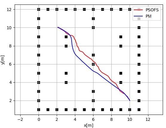
E3S Web of Conferences 270, 01035 (2021) https://doi.org/10.1051/e3sconf/202127001035
WFCES 2021
effectiveness of the use of RS in tasks involving autonomous operation for a long time (for
example, exploration of large areas) or performance of work in aggressive environments
(under water, in space, in areas of radiation contamination). For the effective implementation
of the assigned tasks, such RS must have a high degree of autonomy, which, in turn, leads to
the emergence of a number of specific management problems. Based on the analysis of
research works [1–5], one of the key problems arising during the operation of mobile robots
(MR) in an unknown environment is the planning of safe trajectories of movement, allowing
to build accident-free routes close to optimal (shortest).
The approaches used to solve the problem of planning the trajectory of movement can be
conditionally divided into 2 main groups:
1) classical search algorithms - Dijkstra's algorithm, depth-first search, A*, graph search
methods [6–8];
2) intelligent algorithms - artificial neural networks, fuzzy and genetic algorithms, the main
advantage of which is the speed of calculation with a moderate load on the on-board
computing devices of robots [9–11].
In the course of the analysis, it was revealed that current research in the field of mobile
robotics is aimed at increasing the efficiency of performing target tasks of robots through
their group application, which focuses the main efforts of the authors on solving
communication problems and distributing tasks in MR groups [12,13]. This trend leads to an
obvious complication of the MR control system, while these approaches do not take into
account the specifics of the on-board MR systems: the computational capabilities of control
devices, limited range of sensors and sensors, the speed of reaction to external disturbances,
etc. This fact imposes a number of restrictions on the use of well-known methods for planning
the trajectory of movement when the robot operates in a non-deterministic environment. An
obvious solution to this problem is to reduce the computational complexity of the motion
planning algorithm, taking into account the limited capabilities (sensor and computational)
of mobile robots.
The method described in article [14] is considered as an analogue in this work. This
method is a combination of the particle swarm optimization (PSO) algorithm [15] and the
Fringe Search (FS) algorithm [16]. The main idea of the method is an iterative search for
trajectory control points, taking into account the presence of obstacles, the distance to the
target, the smoothness of the trajectory, and the distance to obstacles are used as efficiency
criteria. The sequence of solving the trajectory planning problem using this method can be
described as follows. First, a reference point is searched in the direction of the target using
PSO. A group of i particles is initialized in a random way, after which, during the execution
of a given number of iterations, an optimal solution is found. At each iteration, the particles
update their position based on two parameters: pi - the best known position of particle i; g is
the best known state of the whole swarm. When the optimal values of pi and g are found, the
particle velocities are updated using the formula:
vi cinvi ccogU (0,1)[ri xi ] csocU (0,1)[ pi xi ],
where vi – is the particle's velocity vector, ri – is the best position found by the particle, pi – is the best
position found by all the swarm particles, xi – is the current position of the particle, the U function
returns a random number from 0 to 1, inclusive, the coefficients ccog and csoc determine the significance
for the particle of its own the best position and the best position among the whole swarm, the coefficient
cin characterizes the inertial properties of the particles.
After calculating the speed of the particles, their location is calculated:
xi xi vi .
If the distance from the found control point to the obstacle is less than the specified one,
then a repeated search is performed using the FS algorithm, which finds the path with the
lowest cost from the current node n to intermediate nodes n'. The list of nodes is calculated
by cell decomposition of a known part of the environment. It is also assumed that the
2E3S Web of Conferences 270, 01035 (2021) https://doi.org/10.1051/e3sconf/202127001035
WFCES 2021
characteristics of obstacles (side lengths and their coordinates) can be determined when the
obstacle first hits the robot's field of view. The cost of the path f to each of the intermediate
nodes is estimated by the formula:
f g h,
where g – is the estimated cost of the path, h – is the estimated distance to the target point.
The simulation results demonstrate the high efficiency of this method for planning a safe
trajectory of the robot's movement. However, the authors do not take into account the range
of on-board sensors and sensors, which significantly limits the field of visibility of the robot;
as a result, it is impossible to accurately identify the characteristics of the obstacle that the
robot encounters during the movement.
Based on the analysis of existing solutions, it can be concluded that the development of a
method for planning the trajectory of a mobile robot, taking into account the limited
capabilities of the on-board system, is an urgent and timely task.
2 Formulation of the problem
The paper considers a two-wheeled mobile robot with a differential drive, the kinematic
scheme of which is shown in Figure 1.
y
v
rw
ѳ
B
w
x
Fig. 1. Kinematic scheme of a mobile robot.
On Figure 1 x and y denote the position of the center of the robot axis in the global
coordinate system, θ indicates the direction of movement of the mobile robot relative to the
x-axis in the global coordinate system. Variable rw is robot’s wheel radius, B – is the distance
between the wheels. Finally, v and w are the linear and angular velocities, respectively, and
wL and wR – are the rotational speeds of the left and right wheels, respectively.
This model in the global coordinate system is one of the simplest and most minimalistic
representations of a two-wheeled mobile robot. In this model, the robot is represented by
three degrees of freedom with a vector:
q [ x, y, ].
The mathematical model of MR can be represented as:
x v cos ,
(1)
y v sin .
The relationship between the linear and angular velocity and the speeds of each of the
wheels can be expressed as follows:
3E3S Web of Conferences 270, 01035 (2021) https://doi.org/10.1051/e3sconf/202127001035
WFCES 2021
rw
v ( wR wL ),
2 (2)
r
w w ( wR wL ).
2
Substituting equations (1) into expression (2), we obtain the following kinematic model
of the robot [17]:
rw
x cos ( wR wL ) ,
2
r
y sin ( wR wL ) w ,
2
rw
( wR wL ).
B
This paper makes a number of the following assumptions:
the mobile robot is equipped with an on-board control device and distance sensors
(lidar);
the mobile robot has a limited field of view b, which can be represented as a circle of a
given radius rb with a center coinciding with the position of the robot. Data on the
presence of obstacles oi∈O, received from distance sensors, is carried out only in the
robot’s field of visibility b;
unknown closed environment means a situation when the boundaries of the robot's
working area are also considered obstacles;
in the global coordinate system, the position of the target point xg,yg, as well as the robot's
own coordinates x(t),y(t) at the current time moment t, are known.
The process of planning the movement of the MR is proposed to be considered as a
problem of step-by-step optimization of the current position of the robot x(t), y(t) relative to
the target point xg, yg. We assume that the time t changes discretely and takes integer values
0, 1, …, k, which are the intervals between adjacent discrete moments of response of the on-
board control device of the robot.
A vector, the components of which are the coordinates of the current position in the global
coordinate system and the angle of rotation, describes the state of the robot:
s(t ) x(t ), y(t ), (t ). (3)
At each moment of time t, the robot is subjected to a control action by means of a control
vector, the components of which are the linear and angular velocities of the robot:
u(t ) v(t ), w(t ). (4)
Thus, at each moment of time t the state of the system is characterized by the vector s(t),
and the control action is characterized by the vector u(t). Under the influence of the control
chosen at the moment t (the decision made), the system passes at the next moment of time to
a new state. The relationship between expressions (3) and (4) can be described by the
relationship:
s(t ) f s t 1 , u t ,t 0,1,..., k. (5)
The distance, which is characterized by the difference between the coordinates of the
robot at the current and previous steps t and t-1 respectively, will be called the trajectory
segment. Then the total length of the trajectory traversed by the robot when moving to the
target can be represented as the sum of the trajectory segments that must be traversed at each
step:
4E3S Web of Conferences 270, 01035 (2021) https://doi.org/10.1051/e3sconf/202127001035
WFCES 2021
Y ft ft 1 ... f k . (6)
In order to prevent collisions with obstacles, restrictions are imposed on the position of
the robot:
si oi o , (7)
where ∆o – is the minimum allowable distance between the robot and the obstacle in the field of
visibility b of the robot.
As an indicator of efficiency, we take the length of the trajectory required to move the
robot from the initial position to the target position. Substituting expressions (5) into (6), we
obtain the additive objective function:
k
Y f k s t 1 , u t . (8)
t 1
Thus, the problem of step-by-step optimization of the process of planning the trajectory
of a mobile robot in an unknown closed environment with obstacles can be formulated as
follows: define for the robot a set of controls u(1), u(2), … , u(k), that transfer the system
from the initial state s(0) to the final state s(k) subject to constraints (7) so that the objective
function (8) reaches a minimum:
Y min.
3 A method for planning the trajectory of a mobile robot in an
unknown closed environment with obstacles
The essence of the proposed method for planning the trajectory of a mobile robot is as
follows. At the beginning, the measurements of the distance sensors are read, which can be
written as a vector:
L(t ) [l1 , l2 ,..., lm ], (9)
where m – is the number of distance sensors installed on the body of each of the robots at an angle α
from each other. It is assumed that one of the lm sensors measures the distance to the obstacle in the
direction coinciding with the orientation of the robot θ (Figure 2).
y lm
l7 l1
ѳi
l2
l6 α
l5 l3
l4
x
Fig. 2. Illustration of the location of the distance sensors.
The angles θm, defining the direction of measurement of distance sensors can be
calculated as follows:
360
m . (10)
m*a
5E3S Web of Conferences 270, 01035 (2021) https://doi.org/10.1051/e3sconf/202127001035
WFCES 2021
Using the data obtained from the distance sensors, it is possible to calculate the possibility
of the robot moving to the point pi, located at a certain distance h in each of the directions θm,
calculated by the formula (10):
( xg xm ) ( yg ym ) ,
2 2
dm (11)
dm : dm dm1 pi xm , ym . (12)
Then, using the PID controller [18], calculate the control vector for the robot:
u(t ) k p * e(t ) ki * e(t )dt kd * z (t ) z (t 1) ,
where kp – is the proportional factor of the regulator, ki – is the integral factor, kd – is the differential
factor, e(t) – is the error signal, z(t) – is the current value of the output signal, z(t-1) – is the previous
value of the output signal.
Thus, a flowchart of the above procedure for control selection is shown in Figure 3.
Start
Reading distance sensor values
For each of the directions:
Calculation of an intermediate position
If the distance to the target
No less current
Yes
Calculation of linear and angular
velocities
Finish
Fig. 3. Block diagram of the proposed method.
According to the review carried out in [2], the most objective criteria for evaluating the
trajectory of a robot are the length and smoothness of the trajectory, as well as its safety - the
distance to obstacles.
The trajectory length is the total distance traveled by the robot from the starting point to
the target. Mathematically, this criterion consists in finding the distance between two points,
which is calculated using formula (11). The shorter the path, the less time it takes for the
robot to move from the start point to the end point.
The smoothness of the trajectory can be defined as the average of the angles of rotation
that the robot needs to make when moving from the start point to the end point.
Mathematically, this criterion consists in determining the angle between two lines using the
formula shown in equation (13). In addition, before finding the angle between any two lines,
the angles of rotation are calculated using the formula shown in equation (14). Finally, the
average value of the angle of rotation for estimating the smoothness of the trajectory can be
found from formula (15). A smaller average angle means that the trajectory is fairly smooth
6E3S Web of Conferences 270, 01035 (2021) https://doi.org/10.1051/e3sconf/202127001035
WFCES 2021
so that the robot can move from the start point to the end point without making too many
turns, especially tight turns.
p(t ) p(t 1)
tan , (13)
1 p(t )* p(t 1)
y (t ) y (t 1)
p , (14)
x(t ) x(t 1)
1 k 1 k
arctg
k t 1
sin (t ), cos (t ) .
k t 1
(15)
Trajectory safety assessment is to calculate the shortest distance from the robot to
obstacles. The shortest distance to obstacles can be obtained based on measurements of
distance sensors according to expression (10):
lmin arg min L(t ) ,
lobs lmin lobs lmin .
4 Method simulation results
To test the proposed method, its software implementation in the Python programming
language was performed. The visualization of the trajectory of the MR movement in an
unknown closed environment with obstacles, as well as the formation of graphs to assess the
effectiveness of the proposed method are performed using the Matplotlib library. During the
simulation, a computer with the following characteristics was used: Intel Core i7-8550U
1.8GHz processor, 8Gb RAM. The simulation parameters indicated in Table 1 were used.
The simulation involved a series of experiments of 20 simulations.
Table 1. Simulation parameters.
Parameter name Value
Number of distance sensors m 16
Distance between the wheels of the robot B 0,2 m
Wheel radius rw 0,04 m
PID proportional gain kp 1
PID integral gain ki 0,01
Differential gain of the PID controller kd 0,1
Maximum travel speed v 0,4 m/s
7E3S Web of Conferences 270, 01035 (2021) https://doi.org/10.1051/e3sconf/202127001035
WFCES 2021
Start point coordinates (10, 2)
Target point coordinates (2, 10)
Minimum distance to obstacles ∆o 1,2 m
Area of visibility b 3m
An example of trajectories obtained by modeling the movement of work using the
proposed method (PM) and the analog method (PSOFS) are presented in Figure 4 (these
designations of the methods will be used further).
Fig. 4. Visualization of the trajectories of the mobile robot in comparison with the analog method.
As can be seen from Figure 4, the characteristics of the obtained trajectories are close to
each other, which is also confirmed by the graphs reflecting the averaged results of 20
experiments. The results are graphically presented in Figure 5.
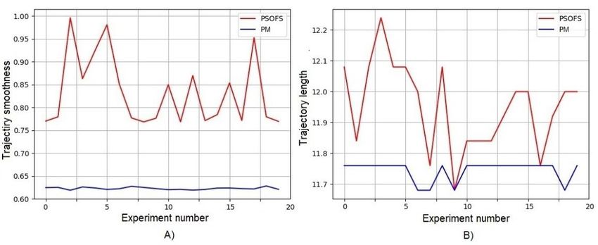
Fig. 5. Simulation results: A) Smoothness of the trajectory of the mobile robot; B) The length of the
trajectory of the mobile robot.
The average value of the trajectory length of 11,74 for the proposed method means that,
on average, for 20 experiments, the total distance traveled by the robot from the starting point
to the target was 11,74 m. The smoothness of the trajectory of 0,62 means that the path is
8E3S Web of Conferences 270, 01035 (2021) https://doi.org/10.1051/e3sconf/202127001035
WFCES 2021
smooth enough for the robot to move from starting point to target without making too many
turns, especially tight turns. Path safety 1,2 means that the shortest distance from the robot
to any of the obstacles is at least 1,2 m. For comparison with the analogous method, the
maximum and minimum values of the trajectory planning quality indicators presented in
Table 2 are also of interest.
Table 2. Comparison of trajectory planning quality indicators for one mobile robot using the
proposed method and the PSOFS method.
Criterion PSOFS PM
Distance traveled
Maximum value 12,23 11,76
Mean value 11,95 11,74
Minimum value 11,68 11,68
Smoothness of the trajectory
Maximum value 0,99 0,63
Mean value 0,83 0,62
Minimum value 0,76 0,61
Distance to obstacles
Total value 1,2 1,2
According to the data presented in Table 2, the proposed method allows generating almost
equal length trajectories of the robot's movement (with a difference of up to 0,47 m in favor
of the proposed method). However, the difference in the smoothness of the trajectory (from
0,15 to 0,36 in favor of the proposed method) indicates that the resulting trajectory has fewer
sharp turns, respectively, the angular velocity of the robot will change less and, as a
consequence, the time spent on the movement will be less. The gain in the smoothness of the
trajectory can be explained by the fact that the proposed method lacks a stochastic component
(the coefficients ccog and csoc in the PSOFS method). The criterion for the safe movement of
the robot relative to obstacles was equal (1,2 m) for the methods under consideration.
5 Conclusions
The presented method allows planning the trajectory of the MR in an unknown closed
environment with obstacles, taking into account the limited performance of the on-board
sensors and computing devices of the MR. Studies that offer a solution to a similar problem
9E3S Web of Conferences 270, 01035 (2021) https://doi.org/10.1051/e3sconf/202127001035
WFCES 2021
include works [9, 14]. In [9], an approach based on artificial neural networks is used to solve
the trajectory planning problem. The use of this mathematical apparatus imposes significant
restrictions on the minimum system requirements of the MR control device, which excludes
the possibility of implementing the method on devices with limited computing resources (for
example, AVR or STM microcontrollers). Thus, this fact reduces the flexibility of the method
under consideration and limits its applicability.
Based on the method of planning the trajectory of the MR movement, proposed in this
work, it is planned to develop methods and algorithms for monitoring closed areas by the
MR group with the maintenance of a given system in order to maximize the coverage of the
territory by on-board sensors and sensors. Additionally, it is planned to modify the presented
method for the possibility of using it in three-dimensional space. In the future, it is planned
to develop a test bench for conducting semi-natural experiments on the use of the proposed
method and its modifications together with algorithms for simultaneous localization and
mapping.
References
1. A. Zakiev, T. Tsoy, E. Magid, ICR 2018 (2018)
2. H. Zhang, W. Lin, A. Chen, Symmetry, 10 (2018)
3. G. Shakhmametova, N. Yusupova, IFAC-PapersOnLine, 51, 538 (2018)
4. V. Petrenko, F. Tebueva, V. Sychkov, V. Antonov, M. Gurchinsky, Int. J. Mech. Eng.
Technol. 9, 447 (2018)
5. V. Petrenko, F. Tebueva, M. Gurchinsky, V. Antonov, J. Shutova, IOP Conf. Ser. Mater.
Sci. Eng. 450, 42013 (2018)
6. L. Liu, J. Lin, J. Yao, D. He, J. Zheng, J. Huang, P. Shi, Artif. Intell. Things Technol.
Appl. 2021, 1 (2021)
7. P. Hart, N. Nilsson, B. Raphael, IEEE Trans. Syst. Sci. Cybern. 4, 100 (1968)
8. T.-F. Wu, P.-S. Tsai, N.-T. Hu, J.-Y. Chen, Adv. Mech. Eng. 9, 1 (2017)
9. R. Glasius, A. Komoda, S. Gielen, Neural Networks 8, 125 (1995)
10. O. Darintsev, B. Yudintsev, A. Alekseev, D. Bogdanov, A. Migranov, Procedia Comput.
Sci. 150, 687 (2019)
11. C. Ahn, R. Ramakrishna, IEEE Trans. Evol. Comput. 6, 566 (2002)
12. C. Banks, J. Kim, J. Shah, Proceedings of the Thirty-First AAAI Conference on Artificial
Intelligence (2017)
13. O. Sergiyenko, M. Ivanov, V. Tyrsa, V. Kartashov, M. Rivas-López, D. Hernández-
Balbuena, W. Flores-Fuentes, J. Rodríguez-Quiñonez, J. Nieto-Hipólito, W. Hernandez,
A. Tchernykh, Rob. Auton. Syst. 83, 251 (2016)
14. M. Wahab, C. Lee, M. Akbar, F. Hassan, IEEE Access 8, 161805 (2020)
15. R. Poli, J. Kennedy, T. Blackwell, Swarm Intell. 1, 33 (2007)
16. Y. Björnsson, M. Enzenberger, R. Holte, J. Schaeffer, IEEE 2005 Symposium on
Computational Intelligence and Games, CIG’05 (2005)
17. V. Petrenko, F. Tebueva, A. Pavlov, V. Antonov, M. Kochanov, ITIDS 2019 (2019)
18. T. Bräunl, Embedded Robotics (2006)
10You can also read