A method for constructing a global motion path and planning a route for a self-driving vehicle

IOP Conference Series: Materials Science and Engineering

PAPER • OPEN ACCESS

A method for constructing a global motion path and planning a route for
a self-driving vehicle
To cite this article: A A Sinodkin et al 2021 IOP Conf. Ser.: Mater. Sci. Eng. 1086 012003

View the article online for updates and enhancements.

 This content was downloaded from IP address 46.4.80.155 on 26/09/2021 at 02:33

MTTV 2020 IOP Publishing
IOP Conf. Series: Materials Science and Engineering 1086 (2021) 012003 doi:10.1088/1757-899X/1086/1/012003

A method for constructing a global motion path and planning
a route for a self-driving vehicle

 A A Sinodkin 1, T S Evdokimova and M I Tiurikov

 Nizhny Novgorod State Technical University n.a. R.E. Alekseev, Nizhny Novgorod,
 Russian Federation

 E-mail: 1 alexey.sinodkin@gmail.com

 Abstract. The article presents methods for constructing an unmanned vehicle (UV) motion
 path in an environment with obstacles to solve the problem of finding a path for a non-
 holonomic vehicle in an environment with obstacles. A combined approach is described and
 individual components are considered that allow solving the problem of planning a path for a
 non-holonomic vehicle. The practical use example of the combined approach for solving the
 problem of planning the UV path is given.

1. Introduction.
 In the past few years, there has been a growing interest in research and experimentation on
autonomous vehicles, especially self-driving ones. One of the key components of the
unmanned vehicle development is planning and searchinga path to a specific goal. When
driving autonomous vehicles, the peculiarity of their movement as non-holonomic systems
should be taken into account. A non-holonomic vehicle’s state can be described in three
dimensions: the vehicle’s two-dimensional position and its driving direction. The 2D position
defines the vehicle coordinates in the environment and the driving path indicates the direction
the vehicle is heading. A simple way to describe this non-holonomic nature is to say that a
vehicle cannot spin on the spot: it cannot change its direction without changing its position.
Classical methods based on cellular decomposition have a number of drawbacks associated
with developing a pathway for vehicles with a vehicle kinematics, and require improvement
[1]. In order to function properly, modern trajectory planning techniques must be able to
detect safe trajectories that correctly account for the limitations inherent in vehicle dynamic
performance.
 Another problem with route planning for non-holonomic vehicles is that the UV moves
along a continuous path, i.e. exists in a continuous environment. Standard methods of path
planning based on cellular decomposition cannot ensure correct path planning in the real
world without significantly increasing computational time. Additionally, the vehicle cannot
navigate the discrete path that the cellular decomposition path planner would detect. As a
result, it is required to consider several methods to form a non-standard (combined) approach,
which should take into account the running time algorithm for constructing the UV trajectory
movement and develop a safe movement trajectory.

 Content from this work may be used under the terms of the Creative Commons Attribution 3.0 licence. Any further distribution
 of this work must maintain attribution to the author(s) and the title of the work, journal citation and DOI.
Published under licence by IOP Publishing Ltd 1

MTTV 2020 IOP Publishing
IOP Conf. Series: Materials Science and Engineering 1086 (2021) 012003 doi:10.1088/1757-899X/1086/1/012003

2. Analytical review of modern methods for traffic planning in an environment with
obstacles
Path planning is an important task in the field of mobile robot navigation. When solving the
path planning problem, the following aspects must be considered: the developed path must
pass from the starting point to the given finishing point, the path must ensure the vehicle
(robot) movement as far as possible from potential obstacles. Thirdly, the path must be
optimal in terms of target parameters among all possible paths.
 The problem described above is solved by methods that use the environment map or
describe it using graphs: methods based on a grid basis [2-4]; potential field methods [2, 5-6,
10-11]; optimization methods [2, 7-9]. In many of these methods, the result is a chain of
control points connecting the starting and finishing points, followed by the problem of
smoothing the resulting path.
 To implement algorithms that take into account complex and heterogeneous constraints,
one algorithm or method is not enough; it is necessary to form a combined approach from
various methods of planning the movement path. This approach will allow taking into
account various restrictions when planning the motion route.

3. Combined path planning approach of a self-driving car
When planning the path of an autonomous vehicle, the position is usually represented as a
three-dimensional vector (x, y, θ), where x and y describe the center location of the vehicle’s
rear axle on the global map, and θ is the angle characterizing the vehicle’s movement
direction relative to the x-axis headed along the vehicle axis symmetry, ϕ is the wheels
rotation angle. This 3D state is shown in (Figure 1).
 The path planner will take the starting
 position as input S0 = (x0, y0, θ0) and the final
 position Sf = (xf, yf, θf) and a sequence of vehicle
 positions at the output S0, S1, ..., Sf is obtained.
 The movement trajectory from S0 to Sf can be
 developed on this basis. This trajectory is then
 smoothed using gradient descent, since the
 trajectory obtained from the calculated positions
 (points) will be a polyline, not realizable for the
 vehicle.
 Based on the above, the combined approach
 algorithm of constructing UV movement path
 (Figure. 2) consists of the following stages:
 1. filling the occupancy grid;
 2. making a distances map to obstacles and
 drawing a Voronoy diagram;
 3. UV movement search for the way to the set
 goal;
 4. smoothing the path built by the Hybrid A *
 algorithm;
Figure 1. Three-dimensional state of the vehicle.
 5. UV traveling along the constructed path.

 2

MTTV 2020 IOP Publishing
IOP Conf. Series: Materials Science and Engineering 1086 (2021) 012003 doi:10.1088/1757-899X/1086/1/012003

 Figure 2. Flowchart of the combined approach operation algorithm

 3

MTTV 2020 IOP Publishing
IOP Conf. Series: Materials Science and Engineering 1086 (2021) 012003 doi:10.1088/1757-899X/1086/1/012003

3.1. Filling in the occupancy grid
At the beginning of the path planning procedure, the environment is indexed in the occupancy grid.
This occupancy grid determines which cells (nodes) in the environment are occupied by obstacles and
which are free space. To simulate the occupancy grid, obstacles are projected onto the grid using the
Bresenham algorithm. According to this algorithm, at each step, one of the coordinates - either x or y
(depending on the angle of segment inclination) changes by one, the change in the other coordinate
(by zero or one) is determined during operation and depends on the error value, the distance at which
actually the installed cell is from the line. Thus, the pixel closer to the ideal segment is selected.
Since when implementing the algorithm it is more convenient to analyze not the error value, but its
sign, the true error value is shifted by -0.5.

3.2. Making a map of distances to obstacles and drawing a Voronoi diagram
A simple occupancy grid is not enough to find a safe path to avoid obstacles. The disadvantage of the
grid is that the path planner will prefer paths that are dangerously close to obstacles as has been shown
above in order to minimize path length. One of the ways to determine the trade-off between path
length and proximity to obstacles is to use the potential field. The potential field can be used to
increase the occupancy grid so that each cell has a calculated cost based on the distance to the
obstacle. Cells that are closer to obstacles have a higher cost of passing; cells that are occupied by
obstacles have an infinite cost. Costs of passing a potential field are used to bypass obstacles remotely
when searching for the best route.
 While the standard potential fields define the cost of passing a cell as a function of the distance to
the nearest obstacle, in this paper an algorithm that uses a combination of the potential fields’ method
and Voronoi diagram to develope the Voronoi field will be used. It determines the cost of passing as a
function of the distance to the nearest obstacle and the distance to the nearest Voronoi edge.
 The key advantage of the Voronoi field over ordinary potential fields is that the field value is
scaled in proportion to the total available distance between obstacles as a result of this even
bottlenecks remain passable, which is not always possible with standard potential field methods.

3.3. UV movement search for the way to the set goal
Pathway planners use cell-based decomposition techniques, such as the A * algorithm commonly used
in robotic pathfinding. The search algorithm applies a grid to the local vehicle environment and
associates the vehicle position with each grid cell when searching.
 However, the A * algorithm is not suitable for solving the problem of path planning for a vehicle,
because the kinematics of the vehicle does not allow it to make turns around its axis. To solve the
described problem, there is a special algorithm developed on the basis of A *. This algorithm was
named Hybrid A *, which allows to take into account the vehicle kinematics.
 Hybrid A * is a variant of the standard A * algorithm based on the cell decomposition method,
which has been redesigned to solve the problem of finding a path at nodes, where path estimation is
carried out without spinning the object around its axis.
 The path planner searches in space using the state vector (x, y, θ, r), where (x∈R, y∈R) is the global
position of the vehicle rear axle center, (θ∈ [-π, π]) is the vehicle direction relative to the x-axis, and
(r∈ {0,1}) - represents the current direction of vehicle movement (moving forward - 0 or moving
backward - 1).
 All nodes found during a Hybrid A * lookup are added to the cell cost priority queue, where the
node cost is calculated using (1):
 ( ) = ( ) + ℎ( ), (1)
where n is the next node on the path, g (n) is the cost of the path from the starting node to the node n,
and h (n) is a heuristic function that estimates the cost of the cheapest path from node n to the target.
The cost of the path g (j) at node j is calculated using the formula (2):
 ( ) = ( ) + (1 + ∙ + ∙ ) + ∙ ℎ , (2)

 4

MTTV 2020 IOP Publishing
IOP Conf. Series: Materials Science and Engineering 1086 (2021) 012003 doi:10.1088/1757-899X/1086/1/012003

where i is the parent node in relation to j; j - child node in relation to i ; dij - Euclidean distance
between nodes i and j; revj - direction of movement of the vehicle at node j (when revj = 1, reverse
movement is performed, revj = 0 - forward direction of movement); vorj - cost at node j of the
Voronoi field; switchij is a change in the direction of movement (for switchij = 1, the directions of the
vehicle's movements at node i and j are different, for switchij = 0 the directions of the vehicle's
movements at node i and j are the same); v, ρ, σ - constant penalty coefficients determining how much
each term affects the cost of the path.
 The cost at the vorj node pushes the construction of a path from obstacles to the edges of the
Voronoi diagram (i.e., to transport corridors where the vehicle can safely pass). The reversing value
rev is the total cost that penalizes the reversing paths, since reversing is a priori slower and more
dangerous than forward. The switch shift value penalizes frequent changes in direction of travel in
order to account for the time it takes to stop completely and change gear [8].
 The second term h(n) of f(n) is an admissible heuristic function that estimates the cost of the path
from node n to the final cell of the path. The heuristic function is calculated using the following
formula (3):
 2 2
 ℎ( ) = √( − ) + ( − ) (3)
where, xi, yi - coordinates of the parent cell; xg, yg - coordinates of the target cell.
 To smooth the path made by the Hybrid A * algorithm, gradient descent is used to minimize the
following objective function (4) [1,12]:
 
 ( ) = ∑ ( , ) + ∑ (| − | − ) +
 =1 =1 (4)
 −1 −1
 ∆ 
 + ∑ ( − ) + ∑(∆ +1 − ∆ )2
 |∆ |
 =1 =1
where Xi = (xi, yi), i ∈ [1, N] is the sequence of vertices, oi is the location of the obstacle closest to the
 ∆ ∆ 
cell;∆Xi = Xi-Xi-1 is the vector of displacement into the cell, ∆ = | ( +1 ) − ( )|-
 ∆ +1 ∆ 
change in the tangential angle in the cell, ρV - the value of the Voronoi field in the cell; kmax -
maximum permissible curvature, limited by the turning radius of the vehicle; dmax - maximum
distance of the collision field with an obstacle; and also ωρ, ωo, ωk, ωs are weight constants.

3.4 UV motion algorithm along the constructed path
At this stage, segments of the movement trajectory in the forward and reverse directions are
constructed, based on the calculated data obtained by the Hybrid A * algorithm operation and the
movement speeds on these path segments are also calculated. Then the algorithm checks whether the
vehicle has reached the final point of the path and, at the same time, as the vehicle moves, calculates
the deviation of the vehicle from the nominal trajectory developed by the algorithm, and corrects the
direction.
 To control the vehicle along the movement trajectory, a PID controller is used to determine the
desired angle of rotation of the wheels δ, due to the received error e, to correct the trajectory. The
wheel turning angle δ is determined by the formula (5):
 
 ( ) = + + = ( ) + ∫ ( ) + , (5)
 
 0
where, e is the closest distance between the nominal track and the vehicle.
 To implement the PID controller in vehicle control, the maximum steering wheel angle must be
observed. It means that δ (t) ∈ [δmin, δmax], the minimum and maximum values of wheel rotation are
set based on the vehicle characteristics.

 5

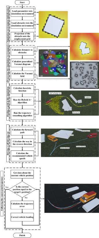
MTTV 2020 IOP Publishing
IOP Conf. Series: Materials Science and Engineering 1086 (2021) 012003 doi:10.1088/1757-899X/1086/1/012003

 To ensure the vehicle smooth running, the movement speed in each cell (node) of the track is
calculated. Each cell in the constructed path has a corresponding recommended speed.
 The recommended vehicle speed at each path point, during the simulation, was determined using
the speed controller based on three parameters: the global speed limit, the instantaneous curvature of
the path in a specific cell, and the deceleration limit based on the speed of subsequent states in the
constructed path.
 The global speed limit exists in all cells of the path, regardless of the peculiarities of each cell and
is set during the simulation by the operator.
 The recommended curvature speed for each waypoint can be calculated using equation (6):
 ‖∆ ‖
 = √ , (6)
 ∆ ∆ 
 |arctan (∆ +1 ) − arctan(∆ )|
 +1 
where, ∆xi = xi-xi-1 is the displacement vector at the i point of the trajectory; amax is the maximum
lateral acceleration that the vehicle can achieve when driving on a curve.
 Because of this lateral acceleration, the vehicle is forced to decelerate during tight bends on the
trajectory. A maximum lateral acceleration of 0.5 m/s 2 was set in the simulation.
 It is not enough to limit speed on steep curves; the vehicle must slow down before it enters a bend
in order to track the correct speed in the right place. To decelerate the vehicle while driving on slow
sections, a deceleration limitation is imposed on the path. The following kinematic equation (7) shows
how the deceleration limiting speed for node i is calculated:
 зам ( ) = √ −1 2 + 2 зам Δ , (7)
where, vi-1 - speed in the current cell; v зам- recommended deceleration speed; aзам - acceleration of
deceleration, specified during simulation by the operator; Δx - distance between the current and the
next cell.

4. Practical implementation of the combined approach for constructing the self-driving vehicle
movement trajectory
Unity, a cross-platform computer game development environment, was chosen to test the operation of
the algorithm. The tests were carried out in a full-scale virtual environment, replicating real-life
conditions to complete the tasks of finding the safe shortest path to the goal.
 As a vehicle for testing the combined approach, a full-scale model of an all-metal GAZ-A65R32
bus with sensors for obstacle detection and orientation in the environment (Figure 3) was used.

 Figure 3. Bus model GAZ-A65R32 with sensors

 6

MTTV 2020 IOP Publishing
IOP Conf. Series: Materials Science and Engineering 1086 (2021) 012003 doi:10.1088/1757-899X/1086/1/012003

Several virtual experiments have been carried out to check for finding paths of trajectory construction
accuracy. For the tests, two scenes were selected: with a random environment and parking spaces
shown in (Figure 4) and (Figure 5). These environments have been used to represent collision-free
driving through obstacles and accurate parking in parking lots.
 To navigate successfully in high density obstacle environments, the vehicle must find a safe,
controlled path, and the controller must follow the constructed path as closely as possible. The
comfort of vehicle passengers is also important so as the vehicle path must be smooth and free from
frequent changes in direction. The speed of calculating the search for a suitable route should not be
high in order to provide only a small delay between the moment when the target is selected and the
vehicle starts moving towards it.

Figure 4. Simulation environment for testing Figure 5. Simulation environment for testing in a
automatic parking random environment

The start and position of each environment was the same; only the positions, sizes and orientations of
100 obstacles were random. Table 1 shows the runtime results for each step in the path planning
process. Generalized Voronoi's chart summarizing is the time required to load all obstacles into the
obstacle grid, summarize a generalized Voronoi's chart and calculate Voronoi's field. The heuristic
clculation is the time required to compute the "holonomic with obstacles" heuristic. The Hybrid A *
runtime is the time it takes to find a path in the environment. The number of nodes extended for each
A * search is also shown. Path smoothing time measures how long it took to smooth the path found
by the Hybrid A *.

Table 1. Runtime of the path planning algorithm for a simulation environment with a random
environment
Stages of the algorithm Simulation environment with Simulation environment with
 random environment (sec) parking spaces (sec)
GVC summarizing 0,391 0,375
Heuristic calculation 0,016 0,004
Hybrid A * operation 0,516 0,328
Smoothing path 0,344 0,031
Total time 1,267 0,738

 7

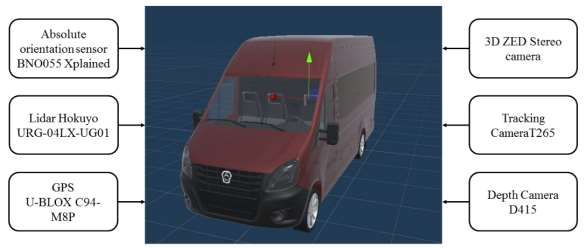
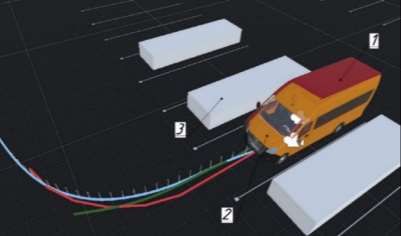
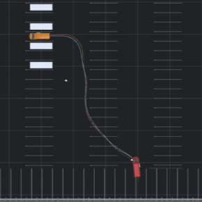
MTTV 2020 IOP Publishing
IOP Conf. Series: Materials Science and Engineering 1086 (2021) 012003 doi:10.1088/1757-899X/1086/1/012003

In order to successfully navigate around densely spaced obstacles with minimal discomfort for
passengers, the desired path must be properly smoothed. Table 2 shows the results for the paths
developed by the Hybrid A * algorithm, and subsequently smoothed, as well as the results if the
constructed vehicle path is polyline.
Table 2. Statistics of overcoming the path along the smoothed and polyline path.
Motion parameters Simulation environment with Simulation environment with
 random environment parking spaces
 Smoothed Polyline Smoothed Polyline
 trajectory trajectory trajectory trajectory
Travel time 64 sec. 77 sec. 22 sec. 24 sec.
Average travel speed 16 km/h 11 km/h 8 km/h 7 km/h
Number of direction corrections 8 pieces. 27 pieces. 3 pieces. 12 pieces.
on the trajectory

The positioning accuracy for the vehicle in free terrain was from 50 mm to 250 mm. In order to
perform the task at hand in parking conditions, the vehicle's control controller must be able to track the
path accurately, especially in the reverse direction. Since this experiment involves reversing entering a
parking space (Figure 6), the effectiveness of tracking the reverse path directly affects the target error.
As well as in the past testing, data on the Hybrid A * algorithm operation speed presented in Table 1,
and the efficiency of its operation when smoothing the broken path developed by the Hybrid A *
algorithm (table 2) were obtained.

 Figure 6. Illustration of the algorithm operation when parking in reverse: 1 - a vehicle parked at a
 given point, 2 - the end point of the path, marked by a static orange vehicle, 3 - an obstacle

The results shown in Table 1 represent an approximate order of magnitude for the time it takes to plan
a path through a moderate-sized environment. This shows that the presented algorithms can be
executed fast enough to provide only a small delay between the moment when the target is selected
and the vehicle starts moving towards it.
 Table 2 shows how track smoothing can affect driving performance as well as travel comfort.
First, when driving on a flat path, the vehicle can smoothly enter corners, which allows increasing the
speed on them. The smoothed trajectory gave a significant increase in the average vehicle speed
compared to the polyline trajectory. Even if the distance from the start to the target was the same in
every randomly generated environment, the vehicle can reach the target in less time when the path is

 8

MTTV 2020 IOP Publishing
IOP Conf. Series: Materials Science and Engineering 1086 (2021) 012003 doi:10.1088/1757-899X/1086/1/012003

smoothed. Second, flattening the desired trajectory provides a much smoother ride for the vehicle's
passengers.
 The accuracy in the studies can be considered satisfactory for driving safely in real conditions and
performing an automatic parking maneuver.

5. Conclusions and Future work
Based on the simulation results, the vehicle positioning accuracy in an environ with a random
environment was from 50 to 250 mm and in an environment with parking spaces from 50 to 105 mm.
The simulation accuracy can be considered satisfactory for safe driving in real conditions, and
automatic parking. The described combined approach is universal in terms of its application to
vehicles with different technical parameters (such as overall dimensions; length and width of the
wheelbase; engine power, etc.). The technical characteristics of the vehicle are set at the beginning of
the simulation by the operator. In the future, it was decided to implement a combined approach on a
real unmanned vehicle based on the GAZ A65R32 vehicle as part of the annual field tests of
unmanned robotic systems "RoboCross".

6. Recommendations
As a recommendation for further work, it is worth noting the need to finalize the terrain maps in the
Unity simulation environment for specific tasks for testing a self-driving vehicle: vehicle movement in
an urban environment, on highways, and over rough terrain.

References
 [1] Izotova T Yu 2016 Review of algorithms for finding the shortest path in the column New
 information technologies in automated systems 19 pp 341-344
 [2] Liu V 2018 Path planning methods in an environment with obstacles (review) Mathematics and
 mathematical modeling 1 pp15–58.
[3] Sleumer N H and Tschichold–Gurman N 1999 Exact cell decomposition of arrangements used
 for path planning in robotics Zurich: Inst. of Theoretical Computer Science
[4] LaValle S 1998 Rapidly-exploring random trees : a new tool for path planning The annual
 research report
[5] Ge S S and Cui Y J 2000 New potential functions for mobile robot path planning IEEE
 Transactions on Robotics and Automation 16-5 pp 615-620 doi: 10.1109/70.880813
[6] Ren J, McIsaac K A and Patel R V 2006 Modified Newton's method applied to potential field-
 based navigation for mobile robots IEEE Transactions on Robotics 222 pp 384-391 doi:
 10.1109/TRO.2006.870668
[7] Ross I M and Fahroo F A 2002 Perspective on methods for trajectory optimization. AIAA/AAS
 Astrodynamics specialist conf. and exhibit pp 1–7.
[8] Fliess M, Levine J, Martin P and Rouchon P 1995 Flatness and defect of non–linear systems:
 introductory theory and examples Intern. J. of Control 61-6 pp 1327–1361
[9] Culligan K, Valenti M, Kuwata Y and How J P 2007 Three-Dimensional Flight Experiments
 Using On-Line Mixed-Integer Linear Programming Trajectory Optimization American Control
 Conference pp 5322-5327 doi: 10.1109/ACC.2007.4283101
[10] Khatib O 1985 Real-time obstacle avoidance for manipulators and mobile robots Proceedings.
 1985 IEEE International Conference on Robotics and Automation pp 500-505 doi:
 10.1109/ROBOT.1985.1087247
[11] Bounini F, Gingras D, Pollart H and Gruyer D 2017 Modified artificial potential field method
 for online path planning applications 2017 IEEE Intelligent Vehicles Symposium (IV) pp 180-
 185 doi: 10.1109/IVS.2017.7995717
[12] Yang K and Sukkarieh S 2008 3D smooth path planning for a UAV in cluttered natural
 environments 2008 IEEE/RSJ International Conference on Intelligent Robots and Systemspp.
 794-800 doi: 10.1109/IROS.2008.4650637

 9