A prognostic dynamic model applicable to infectious diseases providing easily visualized guides: a case study of COVID 19 in the UK - Nature
←
→
Page content transcription
If your browser does not render page correctly, please read the page content below
www.nature.com/scientificreports
OPEN A prognostic dynamic model
applicable to infectious diseases
providing easily visualized guides:
a case study of COVID‑19 in the UK
Yuxuan Zhang1,6,7, Chen Gong2,7, Dawei Li3,7, Zhi‑Wei Wang4,5, Shengda D. Pu2,
Alex W. Robertson2, Hong Yu6* & John Parrington1*
A reasonable prediction of infectious diseases’ transmission process under different disease control
strategies is an important reference point for policy makers. Here we established a dynamic
transmission model via Python and realized comprehensive regulation of disease control measures.
We classified government interventions into three categories and introduced three parameters as
descriptions for the key points in disease control, these being intraregional growth rate, interregional
communication rate, and detection rate of infectors. Our simulation predicts the infection by COVID-
19 in the UK would be out of control in 73 days without any interventions; at the same time, herd
immunity acquisition will begin from the epicentre. After we introduced government interventions, a
single intervention is effective in disease control but at huge expense, while combined interventions
would be more efficient, among which, enhancing detection number is crucial in the control strategy
for COVID-19. In addition, we calculated requirements for the most effective vaccination strategy
based on infection numbers in a real situation. Our model was programmed with iterative algorithms,
and visualized via cellular automata; it can be applied to similar epidemics in other regions if the basic
parameters are inputted, and is able to synthetically mimic the effect of multiple factors in infectious
disease control.
Coronavirus disease (COVID-19) is an infectious respiratory syndrome caused by severe acute respiratory syn-
drome coronavirus 2 (SARS-CoV-2) and characterised by high overall human-to-human transmission p otential1.
The epidemic rapidly spread regionally at the end of 2019 and subsequent follow on caused a global pandemic and
left the world facing a grave social as well as economic crisis2. Yet until an effective vaccination programme for all
populations or specific medicine to combat COVID-19 is realised, it is likely that the possibility of a resurgence
in contagion will exist so that disease control may become a normal part of everyday life3. In most world regions,
the initial basic reproduction number (R0) of COVID-19 was around 2.2–6.474–9. In comparison, for MERS and
SARS, the overall R 0 values were 0.47 and 0.95, respectively10, indicating that the transmissibility of COVID-19
is up to 10 times higher than that of previous coronavirus-caused infectious respiratory syndromes. In addition,,
the complex epidemiological properties of COVID-19 which include a long infectious period (infectiousness
during the incubation period)11, the existence of asymptomatic infectors who have a similar infection capacity
(30–60%)10,12, a high overall self-healing rate (80%)13, yet clinical severity in a minority of individuals14, have
made the disease different from other antecedent epidemics. As such the unprecedentedly enormous infection
scale and limited healthcare system capacity makes it challenging to formulate a proper disease control strategy
in the COVID-19 era.
Over the last year, many previous epidemic studies have successfully provided insights for understanding,
predicting and simulating the development of COVID-19 from multiple perspectives, such as calculating and
predicting the evolving basic reproduction number4; quantitively predicting epidemiological characteristics10,15;
evaluating particular disease control measures such as social distancing16, controlling m obility17–20; analysing
1
Department of Pharmacology, University of Oxford, Oxford OX1 3QT, UK. 2Department of Materials, University
of Oxford, Parks Road, Oxford OX1 3PH, UK. 3Department of Physics, University of California, San Diego, La
Jolla, CA, USA. 4Computer Science, University of York, York YO10 5GH, UK. 5College of Physics, Jilin University,
Changchun 130012, People’s Republic of China. 6Shanghai Chest Hospital, Shanghai Jiao Tong University,
Shanghai 200030, People’s Republic of China. 7These authors contributed equally: Yuxuan Zhang, Chen Gong and
Dawei Li. *email: yuhongphd@163.com; john.parrington@pharm.ox.ac.uk
Scientific Reports | (2021) 11:8412 | https://doi.org/10.1038/s41598-021-87882-9 1
Vol.:(0123456789)
www.nature.com/scientificreports/
transmission dynamics in special populations such as the elderly, obese individuals, and d iabetics3,21,22; evaluating
various factors affecting disease transmission from urban health, meteorological and geo-environmental perspec-
tives, such as water systems, wind speed, and air pollution23–25; and also forecasting the subsequent impacts on
the social environment and economy26,27. Epidemic models evaluating the effect and efficiency of disease control
measures have provided good reference points for policy m akers5,17,21,28,29, and in this study we aim to establish
such a model to systematically simulate different measures, and with consideration of the special epidemiologi-
cal characteristics. Most of the existing models follow the existing principle of susceptible-infectious-recovered
(SIR)7; here we established a novel infectious-hospitalized-self-heal (IHS) model, with application of an iterative
algorithm; asymptomatic infectors, hospitalized infectors, and self-heal infectors were analysed separately. This
new principle makes our model more applicable to COVID-19 when considering its huge infection scale and
its contagiosity in asymptomatic and pre-symptomatic infectors. With the involvement of some region-specific
parameters such as population density, mobility, and hospital capacity, our model is also flexible for application
to different global regions where COVID-19 is unlikely to follow an identical path15. With the platform of cellular
automata, the simulation results are visualized and accessible. In this article, we simulate the development and
recovery processes in the UK for 100 days since the first outbreak, and we discuss what is the optimum plan for
early-stage disease control, and also the optimal vaccination strategy based on the updated conditions, which
will effectively bring the pandemic to an end.
Results
Dynamic transmission model. In this article we summarised governmental interventions into three key
strategies. First, the intraregional transmission probability has been lowered by protective measures or vac-
cinations, which aim to reduce the possibility of people contracting the disease24,30. Second, the mobility of the
population has been reduced by government-level measures like city lock-down, border sealing, and compul-
sory stay-at-home policies19. Last but not least, healthcare system capacity has been enhanced to make sure as
many patients as possible are quarantined and treated, while enhancement of detection capacity has aided early
detection and immediate i solation31. We introduced interregional communication rate (c) to describe the coeffi-
cient of disease transmission between communities to take the impact of population mobility into consideration.
Initial intraregional growth rate (m) was introduced to describe internal infection among communities, which
indicates the influence of personal protection measures such as keeping a social distance and face covering. Dur-
ing the simulated transmission process, intraregional growth rate (m) changes continuously as it is affected by
patient recovery and thus gain of immunity. Detection rate of infectors (k) was introduced to describe the pos-
sibility of an infector (including asymptomatic and pre-symptomatic individuals) being detected.
N5 (t + 1) = N5 (t) + N2,4,6,8 (t) − 4N5 (t) · c · (1 + m5 (t)) − H5 (t) − S5 (t)
1 − (1 − 4c)th
H5 (t) = N5 (t − th ) · m5 (t − th ) · s · (1 − 4c)th + N2,4,6,8 (t − th ) · m5 (t − th ) · h · c ·
4c
1 − (1 − 4c)ts
S5 (t) = N5 (t − ts ) · m5 (t − ts ) · s · (1 − 4c)ts + N2,4,6,8 (t − ts ) · m5 (t − ts ) · s · c ·
4c
t t
1
m5 (t + 1) = m · 1 − · H5 (i) + S5 (i) + N5 (t)
p5
i=1 i=1
N: Daily infection number, c: Interregional communication coefficient (travel rate over 15 k m2), m: Self-growth
rate (intraregional spreading coefficient), h: General percentage of hospitalization (including death), s: General
percentage of self-healing, th: Average latent period, ts: Average self-heal period, H: Daily hospitalization number,
S: Daily self-healing number, p: Population.
We use cellular automata as a platform of modelling; in cellular automata, cells are arranged as matrixes such
1 2 3
as: 4 5 6; each cell represents a region and people tend to migrate between two adjacent cells (details provided
7 8 9
in Supplementary Information, Fig. S1). In the equations, N5(t + 1) is the daily infection number on day t + 1 in
cell 5, which equals the daily infection number on day t added to the effect of migration in and out, then multi-
plied by the intraregional spreading coefficient, and subtraction of the day’s number going to hospital and self-
healing. The percentage of people who migrate out of a square cell from one side is c, therefore, the percentage
of people who migrate out of a whole square is 4c.
Then we introduce controlled parameters to describe the situation after interventions (details in “Methods”
section). To be realistic, controlled interregional communication rate (cc) and detection rate of infectors (k) are
steady state values while controlled intraregional growth rate (mc) is an initial value varying with the immunity
acquisition number.
Scientific Reports | (2021) 11:8412 | https://doi.org/10.1038/s41598-021-87882-9 2
Vol:.(1234567890)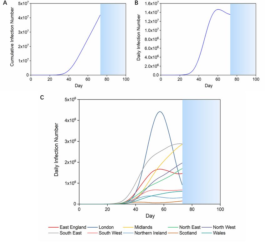
www.nature.com/scientificreports/
N5 (t + 1) = N5 (t) + N2,4,6,8 (t) − 4N5 (t) · cc · (1 + m5 (t)) − H5 (t) − S5 (t) · (1 − k)
1 − (1 − cc )th
H5 (t) = N5 (t − th ) · m5 (t − th ) · h · (1 − cc )th + N2,4,6,8 (t − th ) · m5 (t − th ) · h · cc ·
cc
1 − (1 − cc )ts
S5 (t) = N5 (t − ts ) · m5 (t − ts ) · s · (1 − cc )ts + N2,4,6,8 (t − ts ) · m5 (t − ts ) · s · cc ·
cc
t t
1
m5 (t + 1) = min m · 1 − · H5 (i) + S5 (i) + N5 (t) , mc
p5
i=1 i=1
mc: Initial value of controlled intraregional growth rate, cc: Controlled interregional communication rate, k:
Detection rate of infectors, p: Regional population.
We also take advantage of the definition of m which initially relies on R
0 and changes with the percentage of
immunization to calculate the number of vaccinations required in disease control.
vr + v + i
mc = m · 1 −
p
vr: Required vaccinations, v: Received vaccinations, i: Cumulative number of infections.
Visualised transmission process of COVID‑19 in the UK. Videos showing the prognostic transmis-
sion process on the UK and London maps were generated by Python 3 based on our model (details shown in
“Methods” section and Supplementary Information). Here we present the infection curves (Fig. 1) and visualised
transmission maps (Fig. 2) based on our simulation of the infection which starts with the initial daily infec-
tion number of each region in the UK on 4th March 202032. Due to the limitations of the iterative algorithm,
the earliest date we can start simulating disease control interventions is one day after the first self-heal period.
Therefore, in the first 15 days (a self-heal period) of the simulation, we use the initial parameters according to
COVID-19 epidemiological characteristics, the initial intraregional growth rate as 0.48,33, the interregional travel
rate as 0.138, and the detection rate of infectors as 0 (Table 1, data resources presented in “Methods” section).
Without any governmental intervention, the accumulated infection number in 100 days may exceed 70% of the
UK population (Fig. 1A). Since the simulation was interrupted when the cumulative infection number exceeds
the local population, COVID-19 transmission in the UK suspends on the 73rd day (Fig. 1A). The daily infection
scale will exceed 14.8 million people on the 60th day of domestic infection (Fig. 1B), which accounts for nearly
a quarter of the UK population34. When we look at the regional infection curves, we can see that the epidemic
in London develops differently from other regions in that the infection in the former increases sharply from the
30th to the 58th day, then decreases rapidly (Fig. 1C). This indicates that, without interventions, the infection
will first be eliminated in London while the conditions are still getting worse in other regions.
From the visualized transmission maps we can also see that when the infection peak is reached, the COVID-19
outbreak will ameliorate in the epicentre while it is still developing in surrounding regions (Fig. 2A). As shown in
the screenshots of the simulation videos (Supplementary video files), the epidemic spreads from the epicentre to
the periphery and surprisingly leaves the centre epiclean (Fig. 2A). Here we also simulated the COVID-19 trans-
mission process in London based on the initial daily infection number of each borough on 11th March (Fig. 2B)
which shows similar results32. Despite the fact that a second wave of infection may occur from the epicentre
of the outbreak once again, the periphery may be the place hit by the epidemic more severely in a later period.
COVID‑19 can be brought under control by a single intervention at the early stage, but at
huge expense. We ran simulations to see how effective single interventions are in flattening the daily infec-
tion curves. When the controlled intraregional growth rate (mc) was in the range of 0.05–0.4 (0.75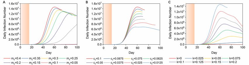
www.nature.com/scientificreports/
Figure 1. Infection curves without interventions in the UK. (A,B) The cumulative/daily infection curve
without interventions in the UK. The simulation stops when cumulative infection number exceeds the regional
population (blue sections). (C) The daily infection curves for regions in the UK without interventions. The
simulation stops when cumulative infection number exceeds the regional population.
20–50% during the COVID-19 lockdowns (January 2020–January 2021)37. Hence, we suppose the interregional
communication rate in the UK to be reduced from 0.1 to 0.08–0.0538, indicating that 20% ~ 32% people can
travel beyond 4 km (2.5 miles) every day. We selected several representative conditions to quantify the UK tier
system, according to this tier system being based on the mobility trends and four-tier alert levels: mc = 0.17
(R0 = 2.5), mc = 0.23 (R0 = 3.5) and mc = 0.3 (R0 = 4.5) with cc in the range of 0.08–0.05 (Table 2)32,35,37; then we
ran simulations and found proper relevant detection rates. The disease control process occurring systematically
with three interventions was simulated and presented as transmission curves (Fig. 4a, b, c). With regard to these
different combinations of interventions, we can conclude that when tier 1, tier 2, and tier 3 lockdown measures
are implemented, the detection rate should be ensured as 16%, 11.5% and 4.5%, and as shown in Fig. 4d, e, f, the
highest daily numbers to hospital (H) under these conditions do not exceed hospital capacity.
Application for calculating vaccination demand to end COVID‑19. A key current strategy to com-
bat COVID-19 is the development of an effective vaccine. We thereby provided a method of calculating the
required vaccination numbers based on this model. We started the simulation with the current infection number
as an initial condition, and intraregional growth rate was influenced by vaccination and existing natural immu-
nity. For example, in early January 2021, the average daily infection cases in the UK were around 35,000 with
3,300 being in London39. Considering the average infection period of COVID-19 which is 2–15 days10, we
assume the real infection number in the UK and London to be 220,000 and 22,00032, accordingly. With the
premise of controlling the pandemic within two months, and controlling m c solely with vaccinations, we simu-
lated the disease control process with the initial infection number of 220,000 and 22,000 in the UK and London
and calculated the required number of vaccinations based on optimized m c values (Fig. 5) by applying the equa-
Scientific Reports | (2021) 11:8412 | https://doi.org/10.1038/s41598-021-87882-9 4
Vol:.(1234567890)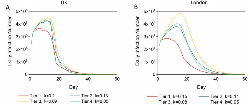
www.nature.com/scientificreports/
Figure 2. Visualized COVID-19 transmission without interventions in the UK and London. (A) Screenshots
of visualized dynamic model of transmission in the UK from day 10 to day 60. The red saturation represents the
severity of COVID-19. COVID-19 starts from a random spot in each region and spreads rapidly. In the outbreak
centre, COVID-19 infection will reach a peak on day 50 and be cleared on day 60 when it is out of control in the
whole country. (B) Screenshots of visualized dynamic model of transmission in London from day 10 to day 90.
(Day-by-day transmission videos were generated by Pythons 3 https://www.python.org using python package
matplotlib https://matplotlib.org with initial maps from open-source software WordPress.org. Screenshots were
generated by Windows10, more details were shown in the Results——Technical details.)
Scientific Reports | (2021) 11:8412 | https://doi.org/10.1038/s41598-021-87882-9 5
Vol.:(0123456789)www.nature.com/scientificreports/
Symbol Definitions Value References
8,33
R0 Basic reproduction number 2.2–6.94
8
m Initial spreading coefficient 0.4
38,42
c Interregional communication coefficient 0.1 (UK)/0.2 (London)
49,50
h Percentage of hospitalization including death rate 0.2
32
s Percentage of self-healing 0.8
18
th Average incubation period 6
46
ts Average self-heal period 15
32
v Received vaccinations (until Jan 2021) 462,114
32
i Cumulative number of infections (until Jan 2021) 3,817,176 (UK)/652,979 (London)
40
R0-D614G Basic reproduction number of variant D614G 3.1–4.8
Table 1. Parameter symbols, definitions and values used as initial conditions in this study.
Figure 3. Impact of single interventions on daily infection curves. (A) Daily infection curves for the UK with
intraregional growth rates varying from 0.4 to 0.05. The orange section means no interventions were taken. (B)
Daily infection curves for the UK with interregional communication rates varying from 0.1 to 0.0125. (C) Daily
infection curves for the UK with detection rates of infectors varying from 0 to 0.2.
tion of mc = m · 1 − vr +v+i
p as presented in an earlier paragraph32. The required number of vaccinations
should be not less than 43 million in the UK and 4.2 million in London (Table 2).
Discussion
As we have summarised, intervention measures have focused on three aspects: the intraregional spreading
rate, detection rate of infectors and interregional communication rate. Long-duration intraregional lockdown
effectively reduced the burden of the pandemic19,20, however, without cutting off the source of infection, the
epidemic will not be eliminated in 100 days, even if the R 0 number is very low (Fig. 3A). With respect to inter-
regional communication rate, during the first round lockdown and associated impact on travel, 46% of driving,
62% of public transport and 33% walking trips, were reduced on the days of lock-down compared to normal
days37. However, the data shows the reduction started from 21st M arch37, when the cases of infection had already
spread all over the country, therefore intraregional growth was already occurring at this p oint35. This also matches
our simulation results and shows that it is difficult to control the infectious trend by simply reducing the travel
parameter once the infection has spread to all regions. We then considered rate of detection and quarantine for
infectors. In our simulation, around one fifth of infectors must be detected and strictly isolated even if they are
in the latent period of the disease or asymptomatic, and enhancing detection rate of infectors (k) is shown to
be the most efficient intervention to bring the infection scale down as well as shorten the intervention period.
However, controlling all the single disease control parameters to ideal values is difficult in real conditions
because of the special characteristics of COVID-19. Detection and isolation of early-stage and asymptomatic
infectors is a big challenge for healthcare systems, and this was particularly the case with the immature detec-
tion technologies and limited resources in the first phase of the COVID-19 o utbreak14,15. Therefore, our findings
support the conclusion that COVID-19 spread must be controlled by multiple combined strategies and as early
as possible (Supplementary Information Fig. S2). The initial R 0 value was around 5.81 in the U K9. To reduce the
social burden as well as balance the needs of the economy and disease control, we believe that controlling R 0
within the range of 2.5–4.5 and mobility reduced by 20–32% (tier 1–3) is a reachable goal with proper control
measures taken at the beginning of the period of interventions17,32,35. To keep the peak daily number of hospi-
talizations within acceptable levels when R 0 is immediately controlled at 2.5 (tier 3), with intermediate travel-
ling control policy, 5% of infectors must be detected and quarantined. When R 0 is controlled at 4.5 (tier 1), our
recommendation is that the detection rate should be enhanced to at least 20%.
Scientific Reports | (2021) 11:8412 | https://doi.org/10.1038/s41598-021-87882-9 6
Vol:.(1234567890)www.nature.com/scientificreports/
Figure 4. Daily infection curve and daily hospitalization curve with combined interventions. m c was in the
range of 0.3–0.17 (initial R0 in the range of 4.5–2.5), and cc was in the range 0.05–0.08 (20–32% people in the
UK can travel over 2.5 miles a day). (A) Daily infection curves when mc was initially controlled at 0.17 ( R0 = 2.5).
(B) Daily infection curves when mc was initially controlled at 0.23 ( R0 = 3.5). (C) Daily infection curves when
mc was initially controlled at 0.3 ( R0 = 4.5). (D) When mc = 0.17, cc = 0.08–0.05, the number to hospital can be
controlled at around 1000 when k is controlled at 0.055–0.045. (E) When mc = 0.23, cc = 0.08–0.05, the number
to hospital can be controlled at around 1000 when k is controlled at 0.105–0.12. (F) When mc = 0.3, cc = 0.08–
0.05, the number to hospital can be controlled around 1000 when k is controlled at 0.16–0.145.
Controlled interregional communication
Restriction level Controlled R0 Controlled intraregional growth rate (mc) rate (cc) Detection rate (k) Vaccinations (million)
London
Tier 4 1.5 0.1 0.05 0.05 4.74
Tier 3 2.5 0.17 0.06 0.08 3.15
Tier 2 3.5 0.23 0.07 0.11 2.21
Tier 1 4.5 0.3 0.08 0.15 0.7
UK
Tier 4 1.5 0.1 0.05 0.05 42.73
Tier 3 2.5 0.17 0.06 0.09 32.85
Tier 2 3.5 0.23 0.07 0.13 28.18
Tier 1 4.5 0.3 0.08 0.2 19.9
Table 2. The detection number and vaccination demand under different intervention levels.
Moreover, our simulation showed that the location at which the epidemic is most severe, was where the epi-
demic first began to disappear. So we suggest that instead of gathering all detection systems and resources to the
main areas affected by the epidemic, distributing these resources to the peripheral regions will be a more efficient
way to save resources and bring the epidemic under control. We also provided a potential method of calculating
required vaccination numbers based on the actual infection number, for example, our simulation shows that
when the infection number is around 220,000 in the UK and 22,000 in London32, the number of vaccinations in
the UK should not be less than 45 million in the UK and 6.6 million in London.
Our study presents a few limitations due to model design as well as the nature of cellular automata. One such
limitation is the inability of cellular automata to mimic long-distance migrations like trips by plane during the
early stage of the disease transmission, as the chroma are only transmitted between two adjacent cells at a time
Scientific Reports | (2021) 11:8412 | https://doi.org/10.1038/s41598-021-87882-9 7
Vol.:(0123456789)www.nature.com/scientificreports/
Figure 5. The daily infection curves at the recovery stage with proper control strategies. (A,B) Ideal daily
infection curves starting with a daily infection number of 220,000 in the UK/22,000 in London.
(Supplementary Information Fig. S1). Another limitation is that mimicking the change of R0 through the process
of viral mutation is not applicable. Future optimizations of such modelling studies may focus on plugging evolv-
ing parameters relating to the variations in the virus in the longer term40. It will also be interesting to introduce
new parameters to quantify other critical factors affecting epidemic transmission from social, economic, envi-
ronmental, demographic, climatological, and health risk a ngles23,25,26,41.
Conclusion
This study is a prognostic analysis of infectious disease development on the strength of an infectious-hospital-
ized-self-heal (IHS) mathematic model with the first wave of COVID-19 in the UK as an example. The model is
designed to match the epidemiological characteristics of infectious diseases with similarities to COVID-19, in
particular ones with asymptomatic and pre-symptomatic infectivity.
Through Python design, we realized the systematic regulation of intraregional growth rate, interregional com-
munication coefficient, and detection rate. It is easy to evaluate the disease control effect by adjusting parameters
and thus we can seek optimal solutions. In addition, we have found that to achieve better control effects in the
mid-term of the epidemic, more attention should be paid to the surrounding areas of the epicentre. Moreover,
our model can also be applied to estimate the quantity of vaccination demand based on realistic situations to
provide guidance for vaccination production.
This model can also be applied in the future to predict the spread of similar infectious diseases in different
regions. It only needs to input specific disease parameters in the system, such as incubation period, self-healing
period, self-healing rate and so on. This model makes it convenient to quickly find the optimal solutions for
comprehensive interventions and take action, which can be helpful in future public health decision-making to
reduce morbidity and mortality.
Methods
Assumptions.
1. The population is approximated to be constant and evenly distributed within each geographical region.
2. Death rate is counted as a part of the percentage of cases that are admitted to hospital.
3. Infected people are contagious constantly from the beginning to the end of the incubation period as well as
during the illness stage.
4. All the population are at the same risk of infection.
5. All patients have contracted the virus through secondary infection; considering the high population mobility,
primary infected patients, which represent a tiny percentage, are omitted.
Automata cell establishment. Cellular automata is a dynamic system that is discrete in time and space;
it consists of a regular grid of cells, with each one being in a finite number of states. In our model, the disease
transmission was described as partial cellular interaction leading to global change. A geographical region was
regarded as a two-dimension network. To input this into cellular automata, each network was deemed as a cell
while each cell stands for the location of a group of people. Pixels were downscaled to correspond to the area of
the cells. Each cell was selected and separated according to the red, green, blue (RGB) value of the map (Supple-
mentary Information Fig. S1). Red colour chromatic value in the pixels represents the severity of the epidemic
in the corresponding regions. The minimum value (r = 0) means no cases while the maximum value (re = 225)
represents the population of the cell.
The epidemic information and regional population of each cell was set i nitially32,34, and the number of people
who migrate each day depends on the interregional communication coefficient and the local population.
Scientific Reports | (2021) 11:8412 | https://doi.org/10.1038/s41598-021-87882-9 8
Vol:.(1234567890)www.nature.com/scientificreports/
A method of convolution kernel was applied for calculation of migrating cases. We suppose that infection
starts from one cell in each region, which was represented as a red dot on the map. The location of the dot was
randomly chosen, and pseudo-random number seeds were fixed. The epidemic is assumed not to transmit to
non-populated areas outside the coast where the infection number was forcibly set as zero.
Dynamical equations. Infectors go to the hospital and become self-healed only after the appearance of
symptoms, and thus the precise number that go to hospital and self-heal depends on the infection number
one period previously. The day’s number to hospital in the cell is dependent on the daily infection number that
occurred six days (the average latent period) previously in local and surrounding regions. Considering that
some infectors will continually migrate between regions, these infectors who are infected 6 days previously and
are currently in cell 5 can be divided into two parts: infectors who were infected in cell 5 and remained in cell 5
(local infectors who never migrate), and infectors who were infected in other cells and moved into the cell 5 in
the previous 6 days. Assuming the number of infectors in cell 5 at the beginning is Y 5.
Day Number of local infectors in cell 5
1 Y5 (1 − 4c)
2 Y5 (1 − 4c)2
3 Y5 (1 − 4c)3
·
·
T Y5 (1 − 4c)t
Therefore, replacing Y with the exact number of infectors, the daily number to hospital of local infectors in
cell 5 on day t is calculated as
N5 (t − th ) · m5 (t − th ) · h · (1 − 4c)th
Next, we consider the number of infectors who move into cell 5. Suppose the number of people in group Y in
adjacent cells of Y5 are Y2, Y4, Y6, Y8, and add up to Y2,4,6,8. Since each cell has only one side in contact with cell 5,
on the first day the number of people in group Y who move into cell 5 is Y2,4,6,8 · c . Meanwhile people also move
out from cell 5, so on the second day the number of people in group Y who move into cell 5 is Y2,4,6,8 · c · (1 − 4c).
The rest can be calculated in the same manner.
Day Number of people in group Y who move into cell 5
1 Y2,4,6,8 · c
2 Y2,4,6,8 · c(1 − 4c)
3 Y2,4,6,8 · c(1 − 4c)2
·
·
t Y2,4,6,8 · c(1 − 4c)t−1
Hence, the total number of people in group Y who move into cell 5 on day t is
t−1
1 − (1 − 4c)t 1 − (1 − 4c)t
Y2,4,6,8 · c(1 − 4c)i = Y2,4,6,8 · c · = Y2,4,6,8 · c ·
1 − (1 − 4c) 4c
i=0
If we replace Y with the exact number of infectors, the daily number of infectors who move into hospital in
cell 5 on day t is calculated as
1 − (1 − 4c)t
N2,4,6,8 (t − th ) · m5 (t − th ) · h · c ·
4c
Therefore, the daily increase in the number of hospitalizations in cell 5 on day t is
1 − (1 − 4c)th
H5 (t) = N5 (t − th ) · m5 (t − th ) · s · (1 − 4c)th + N2,4,6,8 (t − th ) · m5 (t − th ) · h · c ·
4c
In a similar way, the daily increase in the number that self-heal (S) is calculated as
1 − (1 − 4c)ts
S5 (t) = N5 (t − ts ) · m5 (t − ts ) · s · (1 − 4c)ts + N2,4,6,8 (t − ts ) · m5 (t − ts ) · s · c ·
4c
Data sources. We used an initial spreading coefficient to explain the daily percentage increase; in the UK
the initial R0 value was 5.818,9, the infection period (including incubation period) was 15 days, and the incidence
number doubled
every 1.8–2.8 days (Table 1). So the value of the initial growth rate can be calculated as 0.4
m = R0 /15 days .
We set 16,183 pixels, for the areas of the UK. Therefore, on the UK map, each pixel represents a 15 km2 geo-
graphic area, and people who travel over a 4 km (2.5 mile) straight-line distance are considered as migrants. The
percentage of people migrating between cells in the UK is around 40% as roughly estimated based on available
worldwide and domestic travel and transport statistics (Table 1)38,42. Since there are four directions in which
Scientific Reports | (2021) 11:8412 | https://doi.org/10.1038/s41598-021-87882-9 9
Vol.:(0123456789)www.nature.com/scientificreports/
people in one square cell can migrate, the number will be divided by 4, and the travel parameter was estimated
to be 0.1, standing for 10% people in one cell migrating between two adjacent cells every day (Table 1).
The general percentage of hospitalization means the possibility of infectors being accepted to the hospital
and thus strictly isolated. We consulted the cumulative death rate which was estimated at 15.4%, and the number
of beds occupied by confirmed COVID-19 patients according to the NHS statistics in July, which showed that
2000 beds were occupied by COVID-19 patients43. Moreover, in early April the number of hospitalizations was
estimated at around 7000–800044. Considering there to be 200% undetected cases, as the number of undetected
patients is estimated to be more than two times that of the confirmed patients, the percentage to hospital includ-
ing death rate is 20% (Table 1)45.
Since the illness period is estimated at 15 days, the controlled spreading coefficient can be calculated as
m = R0 /15 days, which means the average number of people who can contract COVID-19 from one patient in
one day during his/her illness p eriod46.
The detection rate of infectors stands for the possibility of an infector being detected as well as isolated. For
instance, if the healthcare system provides no detection service, the detection rate of infectors is equal to 0. If
the healthcare system provides enough detection for all patients with severe symptoms and immediately iso-
lates them, the detection rate of infectors is equal to the rate of occurrence of severe symptoms (13.8%)46. If the
healthcare system provides general, extensive and compulsive detection services for all citizens, the detection
rate of infectors will be close to 1.
An approximate validation of the accuracy of the model was based on the early statistics from the UK govern-
ment, although this was hard to do in practice because the real transmission dynamic and infection scale were
difficult to determine at the early stage of the pandemic (Supplementary Table S1).
Technical details. All source codes were generated by Python 3 (https://www.python.org) and Jupyter
Notebook (jupyter.org). Videos were produced by python package matplotlib (https://matplotlib.org) using
"Animation" Class. Initial UK and London maps were downloaded from open-source software WordPress.org
which was released under a General Public License (GPLv2) from the Free Software Foundation47,48, and were
pre-processed by python package scikit-image (https://scikit-image.org) so that all boundaries between regions/
boroughs are smoother for mimicking population migration. All codes are publicly available on GitHub (https://
github.com/daweiliucsd/Cov19-model). In order to run all example codes, prebuilt Python distributions such as
Anaconda are strongly recommended.
Received: 5 October 2020; Accepted: 19 March 2021
References
1. WHO. Report of the WHO-China Joint Mission on Coronavirus Disease 2019 (COVID-19). (2020).
2. WHO. Archived: WHO Timeline—COVID-19. https://www.who.int/news-room/detail/27-04-2020-who-timeline---covid-19.
3. Kissler, S. M., Tedijanto, C., Goldstein, E., Grad, Y. H. & Lipsitch, M. Projecting the transmission dynamics of SARS-CoV-2 through
the postpandemic period. Science (2020). https://doi.org/10.1126/science.abb5793.
4. Chintalapudi, N., Battineni, G., Sagaro, G. G. & Amenta, F. COVID-19 outbreak reproduction number estimations and forecasting
in Marche, Italy. Int. J. Infect. Dis. 96, 327–333 (2020).
5. Koo, J. R. et al. Interventions to mitigate early spread of SARS-CoV-2 in Singapore: a modelling study. Lancet. Infect. Dis 20,
678–688 (2020).
6. Wu, J. T., Leung, K. & Leung, G. M. Nowcasting and forecasting the potential domestic and international spread of the 2019-nCoV
outbreak originating in Wuhan, China: a modelling study. Lancet 395, 689–697 (2020).
7. Gatto, M. et al. Spread and dynamics of the COVID-19 epidemic in Italy: effects of emergency containment measures. Proc Natl
Acad Sci USA 117, 10484–10491 (2020).
8. Sanche, S. et al. High contagiousness and rapid spread of severe acute respiratory syndrome coronavirus 2. Emerg. Infect. Dis. 26,
1470–1477 (2020).
9. Dropkin, G. COVID-19 UK lockdown forecasts and R0. Front. Public Health 8, 256 (2020).
10. Cevik, M. et al. SARS-CoV-2, SARS-CoV, and MERS-CoV viral load dynamics, duration of viral shedding, and infectiousness: a
systematic review and meta-analysis. Lancet Microbe 2, e13–e22 (2021).
11. Linton, N. M. et al. Incubation period and other epidemiological characteristics of 2019 novel coronavirus infections with right
truncation: a statistical analysis of publicly available case data. JCM 9, 538 (2020).
12. Kwok, K. O., Lai, F., Wei, W. I., Wong, S. Y. S. & Tang, J. W. T. Herd immunity—estimating the level required to halt the COVID-19
epidemics in affected countries. J. Infect. 80, e32–e33 (2020).
13. Wilder-Smith, A., Chiew, C. J. & Lee, V. J. Can we contain the COVID-19 outbreak with the same measures as for SARS?. Lancet.
Infect. Dis 20, e102–e107 (2020).
14. Stawicki, S. et al. The 2019–2020 novel coronavirus (severe acute respiratory syndrome coronavirus 2) pandemic: a joint american
college of academic international medicine-world academic council of emergency medicine multidisciplinary COVID-19 working
group consensus paper. J Global Infect Dis 12, 47 (2020).
15. Jewell, N. P., Lewnard, J. A. & Jewell, B. L. Predictive mathematical models of the COVID-19 pandemic: underlying principles and
value of projections. JAMA 323, 1893 (2020).
16. Farboodi, M., Jarosch, G. & Shimer, R. Internal and External Effects of Social Distancing in a Pandemic. w27059 http://www.nber.
org/papers/w27059.pdf (2020). https://doi.org/10.3386/w27059.
17. Li, Y. et al. The impact of policy measures on human mobility, COVID-19 cases, and mortality in the US: a spatiotemporal perspec-
tive. IJERPH 18, 996 (2021).
18. Chang, S. et al. Mobility network models of COVID-19 explain inequities and inform reopening. Nature 589, 82–87 (2021).
19. Imperial College COVID-19 Response Team et al. Estimating the effects of non-pharmaceutical interventions on COVID-19 in
Europe. Nature 584, 257–261 (2020).
Scientific Reports | (2021) 11:8412 | https://doi.org/10.1038/s41598-021-87882-9 10
Vol:.(1234567890)www.nature.com/scientificreports/
20. Islam, N. et al. Physical distancing interventions and incidence of coronavirus disease 2019: natural experiment in 149 countries.
BMJ m2743 (2020). https://doi.org/10.1136/bmj.m2743.
21. Kucharski, A. J. et al. Early dynamics of transmission and control of COVID-19: a mathematical modelling study. Lancet. Infect.
Dis 20, 553–558 (2020).
22. CMMID COVID-19 working group et al. Age-dependent effects in the transmission and control of COVID-19 epidemics. Nat
Med (2020). https://doi.org/10.1038/s41591-020-0962-9.
23. Coccia, M. How do low wind speeds and high levels of air pollution support the spread of COVID-19?. Atmos Pollut Res https://
doi.org/10.1016/j.apr.2020.10.002 (2020).
24. Gormley, M., Aspray, T. J. & Kelly, D. A. COVID-19: mitigating transmission via wastewater plumbing systems. Lancet Glob. Health
8, e643 (2020).
25. Coccia, M. An index to quantify environmental risk of exposure to future epidemics of the COVID-19 and similar viral agents:
Theory and practice. Environ. Res. 191, 110155 (2020).
26. Yang, C. et al. Taking the pulse of COVID-19: a spatiotemporal perspective. Null 13, 1186–1211 (2020).
27. Wolf M. The risks of lifting lockdowns prematurely are very large. Financial Times.
28. Kraemer, M. U. G. et al. The effect of human mobility and control measures on the COVID-19 epidemic in China. Science 368,
493–497 (2020).
29. Prem, K. et al. The effect of control strategies to reduce social mixing on outcomes of the COVID-19 epidemic in Wuhan, China:
a modelling study. Lancet Public Health 5, e261–e270 (2020).
30. Greenhalgh, T., Schmid, M. B., Czypionka, T., Bassler, D. & Gruer, L. Face masks for the public during the covid-19 crisis. BMJ
m1435 (2020). https://doi.org/10.1136/bmj.m1435.
31. Peck, K. R. Early diagnosis and rapid isolation: response to COVID-19 outbreak in Korea. Clinical Microbiology and Infection
S1198743X20302330 (2020). https://doi.org/10.1016/j.cmi.2020.04.025.
32. https://coronavirus.data.gov.uk/. Coronavirus (COVID-19) in the UK.
33. Tang, B. et al. Estimation of the transmission risk of 2019-nCov and its implication for public health interventions. SSRN J. https://
doi.org/10.2139/ssrn.3525558 (2020).
34. Population of England in 2019, by region. https://w ww.s tatis ta.c om/s tatis tics/2 94681/p opula tion-e nglan d-u nited-k ingdo m-u k-r egio
nal/.
35. Hale, T., Petherick, A., Phillips, T. & Webster, S. Variation in government responses to COVID-19. Version 2.0. Blavatnik School
of Government Working Paper.
36. Rees, E. M. et al. COVID-19 length of hospital stay: a systematic review and data synthesis. https://d oi.o
rg/1 0.1 101/2 020.0 4.3 0.2 0084
780 (2020). https://doi.org/10.1101/2020.04.30.20084780.
37. APPLE MAPS. Mobility Trends Reports. https://www.apple.com/covid19/mobility.
38. UK.GOV. Transport Statistics Great Britain: 2019. https://w ww.g ov.u k/g overn ment/s tatis tics/t ransp ort-s tatis tics-g reat-b
ritai n-2 019.
39. Coronavirus (COVID-19) Cases. https://data.london.gov.uk/dataset/coronavirus--covid-19--cases.
40. Volz, E. et al. Evaluating the effects of SARS-CoV-2 spike mutation D614G on transmissibility and pathogenicity. Cell 184, 64-75.
e11 (2021).
41. Coccia, M. Factors determining the diffusion of COVID-19 and suggested strategy to prevent future accelerated viral infectivity
similar to COVID. Sci. Total Environ. 729, 138474 (2020).
42. London Datastore. Coronavirus (COVID-19) Mobility Report. https://data.london.gov.uk/dataset/coronavirus-covid-19-mobil
ity-report.
43. NHS. Bed Availability and Occupancy. https://www.england.nhs.uk/statistics/statistical-work-areas/bed-availability-and-occup
ancy/.
44. NHS. COVID-19 Hospital Activity. https://www.england.nhs.uk/statistics/statistical-work-areas/covid-19-hospital-activity/.
45. Böhning, D., Rocchetti, I., Maruotti, A. & Holling, H. Estimating the undetected infections in the Covid-19 outbreak by harnessing
capture–recapture methods. Int. J. Infect. Dis. 97, 197–201 (2020).
46. Chen, J. et al. Clinical progression of patients with COVID-19 in Shanghai, China. J. Infect. 80, e1–e6 (2020).
47. GNU General Public License, version 2.
48. Interactive UK Map. https://wordpress.org/plugins/interactive-uk-map/.
49. Garg, S. et al. Hospitalization Rates and Characteristics of Patients Hospitalized with Laboratory-Confirmed Coronavirus Disease
2019—COVID-NET, 14 States, March 1–30, 2020. MMWR Morb. Mortal. Wkly. Rep. 69, (2020).
50. Hong, Y.-R., Lawrence, J., Williams, D. & Mainous, A. III. Population-level interest and telehealth capacity of US Hospitals in
Response to COVID-19: cross-sectional analysis of google search and national hospital survey data. JMIR Public Health Surv. 6,
e18961 (2020).
Author contributions
This research was designed by Y.Z. and C.G. with the advice of H.Y. and J.P. D.L., C.G. and Z.W.W. created the
codes. Y.Z. and D.L. ran the simulations. All authors interpreted the results and contributed to the discussion
and manuscript preparation.
Competing interests
The authors declare no competing interests.
Additional information
Supplementary information The online version contains supplementary material available at https://doi.org/
10.1038/s41598-021-87882-9.
Correspondence and requests for materials should be addressed to H.Y. or J.P.
Reprints and permissions information is available at www.nature.com/reprints.
Publisher’s note Springer Nature remains neutral with regard to jurisdictional claims in published maps and
institutional affiliations.
Scientific Reports | (2021) 11:8412 | https://doi.org/10.1038/s41598-021-87882-9 11
Vol.:(0123456789)www.nature.com/scientificreports/
Open Access This article is licensed under a Creative Commons Attribution 4.0 International
License, which permits use, sharing, adaptation, distribution and reproduction in any medium or
format, as long as you give appropriate credit to the original author(s) and the source, provide a link to the
Creative Commons licence, and indicate if changes were made. The images or other third party material in this
article are included in the article’s Creative Commons licence, unless indicated otherwise in a credit line to the
material. If material is not included in the article’s Creative Commons licence and your intended use is not
permitted by statutory regulation or exceeds the permitted use, you will need to obtain permission directly from
the copyright holder. To view a copy of this licence, visit http://creativecommons.org/licenses/by/4.0/.
© The Author(s) 2021
Scientific Reports | (2021) 11:8412 | https://doi.org/10.1038/s41598-021-87882-9 12
Vol:.(1234567890)You can also read