A simple, non-recursive model of the spread of Covid-19 with applications to policy
←
→
Page content transcription
If your browser does not render page correctly, please read the page content below
A simple, non-recursive model of the spread of
Covid-19 with applications to policy
Ernst-Ludwig von Thadden∗
April 16, 2020
Covid-19 “might be a one-in-a-century evidence fiasco"
(J. Ioannidis, STATnews 17/3/20)
1 Introduction
Much of the rapidly developing economic literature on the spread of the Covid-
19 pandemic builds on the classic SIR-model of contagion.1 The simplest version
of this model derives the dynamics of transmission in a recursive framework, in
which the number of newly infectious individuals in a population (∆ or )
depends on the number of non-infected individuals () who are susceptible to an
infection in a reduced-form model of personal encounters.2 At the early stage of
the epidemic where we are currently, the mitigating effect of having increasing
numbers of individuals removed () from the susceptible group through immu-
nization or death can be neglected. Hence, if denotes the number of infectious
individuals and the net transmission rate (per period), then new infections
are = , yielding simple exponential growth.
While the model is a useful basis for longer-run macroeconomic analyses,3
Covid-19 presents (at least) two problems that make an application of the basic
∗ Department of Economics, Universität Mannheim, vthadden@uni-mannheim.de. I am
grateful to Toni Stocker and Carsten Trenkler for advice and to Lukas Mevissen for unwavering
research assistance.
1 The model goes back to Kermack and McKendrick (1927). A timely review of this and
related models is Allen (2017) and, just in time, as I have just learned, Stock (April 5, 2020).
My favorite description is in Brown (1978, Ch. 4).
2 Unfortunately, sometimes the acronym is interpreted as “susceptible-infected-recovered".
This is too narrow, and the original model (e.g., in Brown, 1978) divides the population more
generally in susceptible, infectious, and removed agents. Removal may be recovery, but it is
much broader, as it also includes quarantine and other policy measures. On the other hand,
infectious is narrower than infected. Most applications of the model that I know of, however,
assume that the infected are immediately infectious. The fact that this is not the case with
Covid-19 is one of the aspects of the model developed in this paper.
3 Such as Atkeson (2020) and Eichenbaum, Rebelo, Trabant (2020). This literature grows
like = .
1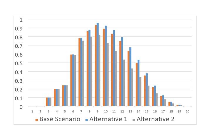
SIR-model difficult for short- and medium-run policy. First, transmission does
not simply depend on the number of infectious, but on the composition of this
group, which is influenced by policy. And second, the data at our disposal are
quite inadequate to evaluate the evolution of the disease and thus the effective-
ness of policy. In fact, in most countries we do not even know the number of
infected, not even their magnitude, let alone that of infectious individuals. This
state is very unsatisfactory, as politicians must make real-time decisions with
dramatic economic and societal consequences based on insufficient data.
This paper presents a simple model that addresses both of these problems by
looking in more detail into the structure of the transmission process. The model
identifies the variables which we need to understand and measure better, estab-
lishes relations between them that can be used to make efficient use of the data
that we can observe, and points to several mechanisms by which policy influ-
ences these variables. The model essentially provides a generalization of the SIR
model in two respects. First, it generalizes the relation = to account
for the structure of the infectious population and introduces the concept of the
“cohort composition kernel" that generalizes the aggregate transmission func-
tion and renders the transmission model non-recursive. Second, it shows how
policy measures such as social distancing, targeted testing or quarantine rules
can affect this kernel and how this can provide estimates for the impact and lag
of non-pharmaceutical policy interventions.
The research presented here is very preliminary and uses data sources until early
April. My emphasis is on policy and, of course, I am most familiar with the
German data and policy. But the structural problem is the same all over Europe
and probably more broadly.4
The model presented here is at the same time much simpler than the influential
model by Ferguson, Cummings et al. (2006) that is the basis for the simulations
recently conducted by Ferguson et al. (March 16, 2020, the “Imperial Study"),
and more detailed in some respects, as it explicitly considers the working of
parameters that can be used for policy. It thus tries to bridge the gap between
the mathematical theories of dynamical systems, the clinical evidence, and the
reduced form models used by economists to evaluate the economic consequences
of the crisis.
2 Individual Evolution of the Disease
Time is discrete, = 0 1 , and measured in days.
4 There is a rapidly growing body of clinical evidence, mostly evaluating small sample
experiences from China in January and February 2020; and not being an expert, I am much
indebted to the summaries provided by the websites of the Centers for Disease Control and
Prevention, its German counterpart, the Robert-Koch Institute, or public discussions by
virologists, such as Christian Drosten of the Charité at Humboldt University. These are, re-
spectively, https://www.cdc.gov/coronavirus/2019-ncov/hcp/clinical-guidance-management-
patients.html, https://www.rki.de/DE/Content/InfAZ/N/Neuartiges_Coronavirus/Steckbrief.html,
and https://www.ndr.de/nachrichten/info/Corona-Podcast-Alle-Folgen-in-der-
Uebersicht,podcastcoronavirus134.html.
2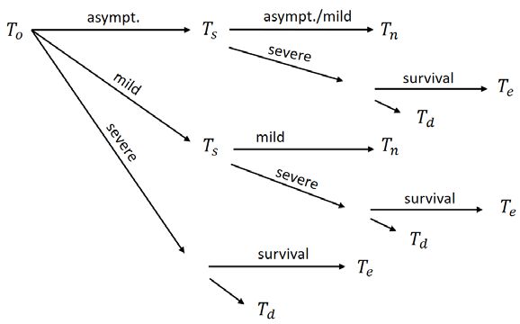
At the individual level, the disease and its consequences evolve in stages after
the infection. Suppose infection is at time = 0. The different stages of the
disease are then given by the following random times , measured in days after
infection.
• (outbreak): time of first clear symptoms (if at all) or undetected out-
break for mild or asymptomatic cases
• = + (no more infectious): time until no more contagious if no
severe symptoms
• = + min( ) (severe): time until severe symptoms if any
• = + (exit): time until end of infection after severe symptoms
• = + (death): time until death after severe symptoms
and the are positive-valued random variables. In case of no clear symp-
toms or no symptoms at all, is an artificial date to make the subsequent
timing comparable.5
The above events refer to the evolution of the disease only, not to any interven-
tions. Diagnoses at the time of outbreak are grouped into three types:
- : asymptomatic (resp., unnoticed by patient)
- : mild, but clear symptoms (fever, cough, etc.)
- : severe, potentially life-threatening (acute respiratory distress (ARD), severe
pneumonia, lung failure, cytokine release syndrome, etc.)
To simplify the presentation, the model does not distinguish between patients
with severe symptoms and critically ill patients. In functioning medical envi-
ronments the former is usually associated with hospitalization,6 the latter with
progression to ICUs. Clinical data from January/February 2020 indicate that
this progression has occured in approximately 30% of all hospitalizations.7
If the individual outbreak immediately produces symptoms, we have = 0, i.e.
= . For asymptomatic and mild cases, we have 0 if severe symptoms
occur later, and = ∞. if not. See Figure 1 for an illustration of the evolution
after the outbreak.
Given the current experience, the following probabilities seem reasonable bench-
mark estimates for the evolution at the time of the initial outbreak, :
= 02 − 04 (1)
= 05 − 06 (2)
= 001 − 002 (3)
5 Completely asymptomatic cases seem to be rare, though. Upon careful investigation,
most patients are able to identify at least some very mild signs (as in the “Munich study" by
Böhmer, Buchholz et al., SSRN preprint 31/3/2020. See Drosten Podcast 24, 30/3).
6 This was different during the early spread of the disease in Wuhan in January, where
hospitalization was also used a isolation device.
7 See Ferguson et al. (Imperial College, 16/3/2020) or Centers for Disease Control and Pre-
vention at https://www.cdc.gov/coronavirus/2019-ncov/hcp/clinical-guidance-management-
patients.html
3Figure 1: The basic dynamics of the virus
Remark: These parameters are highly subgroup-specific (severe cases are heav-
ily concentrated in the over 70 yr group), and sub-group-specific estimates are
strongly biased.8 Furthermore, it is not clear how the probabilities can be es-
timated at all, because the underlying population (all infected individuals) is
unobservable.9 See, e.g., Verity, Okell, Dorigatti et al. (2020) for some discus-
sion of “crude CFRs".
The conditional probability of progressing to severe symptoms from initially no
or mild symptoms is not systematically documented it seems.10 Given estimated
8 This is particularly true for the Wuhan data from January, where the health system was
quickly overwhelmed.
9 There is some important information from natural experiments.
Most impressive is the experiment in Vò (Italy) where the entire population of 3 300 was
tested in late February and then again 10 days later. The findings in Vò seem to be consistent
with ∈ [03 05]. Source: Financial Times, 17/3/20.
A well known natural experiment is the case of the cruiseship Diamond Princess that was
quarantined between Feb. 3 and 20 in Yokohama after a passenger who had disembarked on
Jan. 25 tested positive on Feb. 1. Almost all passengers and crew were tested subsequently,
and 18% of all positive passengers seem to have had no symptoms (Mizumoto et al., 2020).
Given that the average age of passengers was 58, this is consistent with being well above
20% in broader populations. Numbers differ across reports and studies (perhaps because they
were written before the full extent of the data was known). A sufficiently informed (but not
complete) report seems to be https://www.cdc.gov/mmwr/volumes/69/wr/pdfs/mm6912e3-
H.pdf
According to Ferguson et al. (the Imperial Study), Verity, Okell, Dorigatti et al. (MedArxiv,
09/03/2020) find 40 - 50% unrecognized cases on repatriation flights from China in late Jan-
uary. This finding is not reported in the Verity et al. paper, though.
Interesting estimates along the above lines can be obtained by comprehensive tests in special
institutions such as care facilities (see, e.g., Kimball, Arons et al. (2020) for the case of a long-
term care facility in Washington).
1 0 There is signifiant evidence from Wuhan for the clinical progression of Covid-19 during
4overall probabilities of developing severe symptoms eventually, it seems realistic
to put this probability at
= 002 − 005 (4)
Together with (3), (4) gives an interval for the overall probability of severe
symptoms conditional on infection of = + (1 − ) ∈ [003 007].11
A good current estimate for the median incubation period (time until after
infection) seems to be12
= 5 − 6 (5)
with most of the mass on the interval [3 11]. I assume that the events during
the evolution of the disease are i.i.d. across individuals; in other words, the
distributions of all events are not patient specific (while the outcomes are).13
Let = (0 1 2 ) be the (discrete density of the) probability distribution
of outbreak days after infection (over N0 , = 0 is the day of infection).
For patients with mild symptoms at outbreak, severe symptoms are observed,
if at all, days later, with most of the mass on days [5 11] after incubation.14
Let = ( 0 1 2 ) be the corresponding probability distribution.15
For severe cases, probabilities and time to death depend on the clinical environ-
ment and can therefore not be pinned down universally and without reference
hospitalization. This is informative for because in the early phase of the outbreak in Hubei
many patients with relatively mild symptoms were hospitalized. An interesting example is
Zhou, Yu, Du et al. (2020).
1 1 Remember: I do not distinguish between “severe" and “critical". The former is often
associated with hospitalization, the latter with life support on ICUs. But even in published
studies the distinction is not always clear. The estimates given here are on the low side if all
hospitalized cases are included.
Ferguson et al. (16/3/2020, the Imperial Study), building on Verity, Okell, Dorigatti et al.
(2020), give an estimate of 4.4% for , arguing that their original data from China are likely to
be biased. On the “Diamond Princess" 52 of the 697 infected cases developed critically severe
symptoms. These 7.5% are high compared to what one can expect for the general population,
as the overall group on the ship was relatively high risk (and by far most infections occured in
the over-60 age group). Data from Russel et al. (2020), with some preliminary background.
Again, careful: reports such as that until 2/4/2020, "13% of all Covid 19 patients
were hospitalized" (https://www.n-tv.de/infografik/Coronavirus-aktuelle-Zahlen-Daten-zur-
Epidemie-in-Deutschland-Europa-und-der-Welt-article21604983.html) are misleading. The
denominator is wrong.
1 2 See Wall Street Journal, March 9, 2020, https://flexikon.doccheck.com/de/SARS-
CoV-2, https://www.cdc.gov/coronavirus/2019-ncov/hcp/clinical-guidance-management-
patients.html, the references therein and many others in the same ball park.
1 3 This seems to be common in the mathematical epidemiological literature. It is, of course,
possible to condition the distributions on obervable characteristics.
1 4 Relevant data seem to be mostly from Hubei, summarized by Wu, McGoogan
(2020). Early cases in Wuhan were documented by Huang, Wang, Li et al.
(2020). Here and on other topics the documentations by the Robert-Koch-Institute at
https://www.rki.de/DE/Content/InfAZ/N/Neuartiges_Coronavirus/Steckbrief.html and the
CDC at https://www.cdc.gov/coronavirus/2019-ncov/hcp/clinical-guidance-management-
patients.html are most useful.
1 5 I am using the convention that probability distributions over days since infection (the
events ) are denoted by , and those for days since the last event (the incremental lags
) by .
5to specific policy. The Hubei studies of January/February 2020 report mortal-
ity rates of 10 - 25 % conditional on hospitalization.16 In any case, I am less
interested in hospitalization and fatality ratios, because once in hospital, the
dynamics are mechanical (as concerns the spread of the disease).
It is critically important to know when infected patients are contagious. One of
the most striking findings of the early literature is that the virus can be trans-
mitted before an outbreak is noticed.17 The time span over which transmission
can occur is usually stated with reference to the outbreak date and probably
individual-specific, say [ − + ]. Current estimates for the onset of
contagiousness, , suggest values ∈ [0 2].18 For the end date of untreated
cases, + , there seems to be a window of ∈ [6 12] days after the out-
break, with even longer times possible for children.19 This implies that, in the
absence of mass testing, the vast majority of infections occur when the trans-
mitter either is completely unaware of her disposition or has mild symptoms
for which she has not been tested.20 Combined with the evidence for , this
yields an overall broad time interval of [1 23] days after infection, during which
(at least some) individuals can be contagious, with little or no mass on = 1 2
and in the far right tail.
Let = (0 1 2 ) be the probability distribution of the day of the
onset of contagiousness since infection, and = ( 0 1 2 ) the probability
distribution of the final day of infectiousness since incubation, both conditional
on not being quarantined or hospitalized. According to the previous remarks
we should have = 0 for ≥ + 1 and = 0 for ≤ 5.
Remark 1: There does not seem to be much evidence on these distributions.
Probably, they are not independent of each other.21 The papers I have read
usually provide means or medians and estimates of the support (min/max).
This makes it difficult, in particular, to calculate confidence intervals or p-values
in empirical studies.
The following tools from probability theory are useful to put these distributions
to work.
1 6 See Verity, Okell, Dorigatti (2020) and the references therein. They model Case Fatality
Rates (CFRs) and other mortality indicators based on early data.
1 7 See, e.g., https://www.cdc.gov/coronavirus/2019-ncov/hcp/clinical-guidance-
management-patients.html, and the discussion in Section 4 below.
1 8 Ferguson et al. (March 16, 2020, the Imperial Study), assumes a point estimate of =
05, which implies a larger upper bound for the actual distribution of , consistent with other
findings. For evidence, see the discussion in Section 4 below and the references given there.
1 9 See https://www.cdc.gov/coronavirus/2019-ncov/hcp/clinical-guidance-management-
patients.html, https://flexikon.doccheck.com/de/SARS-CoV-2#cite_note-50 and the
references therein. An interesting small sample result is in Wölfel, Corman, Guggemos et al.
(MedRvix 8/3/20; Nature, forthcoming).
2 0 This is currently the case in most countries. South Corea, Taiwan, and Hong Kong seem
to be notable exceptions.
2 1 For example, the distribution of the time from the outbreak of symptoms until exit from
infectiousness ( ) may depend on the day of the outbreak ( ).
6• Cumulative lags: If the distributions of subsequent lags are independent,
the density (probability mass) function of subsequent events can be ob-
tained by the usual convolution of the densities. Example: if the dis-
tribution of days from the onset of infectiousness to incubation is
independent of the distribution of the duration from infection to the
onset of contagiousness , then
X
= − (6)
=0
• Time intervals: Example: The probability that an individual on day
after infection is already contagious (on or past ), but has not yet had
symptoms (before ) is
∞
X
X
Pr( ≤ + ) = − (7)
=+1 =0
Given the evidence cited above, the first sum (summation over ) will not
extend much further than 12 or 13.
3 The Population Dynamics
Capital letters are stocks (end of the day) of current cases, lower case letters
are flows (during day ). Consider a given population (which may be a sub-
population of another population, such as the population of a certain region, or
the above 70-years olds in that region). A key group of interest in the population
is the group of all currently infected individuals, called X , of which there are
(at the end of day ) . The increment during day is ∆ = − −1 . The
size of the inflow into X (the new infections) is X
= . Note that neither
nor ∆ appear in any of the official statistics.
In order to define the subgroups of X that are relevant for policy, we must
consider one important policy variable, testing. I assume that the population
can be tested for the virus and that tests are correct.22 Furthermore, to simplify
the exposition and, in fact, as is the case in all somewhat functioning health
systems, I assume that all severe cases are automatically tested and hospitalized,
and that people only die in hospital.23 Finally, the base model will not consider
mass testing of asymptomatic patients. This can be introduced into this model
fairly easily, but is left for future research. Targeted testing of asymptomatic
individuals based on special tracing procedures is a more elaborate option that
must be modelled explicitly. Hence, the only relevant policy variable explicitly
considered here is the intensity with which patients with mild symptoms are
2 2 This
assumption is not innocuous, in particular in times of extreme stress of the system.
2 3 This
does not mean that all hospitalized cases receive the same treatment. In fact, several
current examples show that the mortality rate in hospitals depends on the hospitalization rate
(however defined).
7tested. Thus the model corresponds to the practice in Germany and many
other European countries until early April (where, of course, the test intensity
has varied across countries and time).
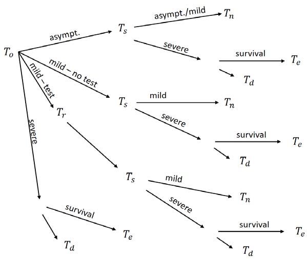
The spread of the infection can be now be described as in Figure 2, which
extends Figure 1. It includes the outcomes “mild - no test" and “mild - test"
after the outbreak date , where the probability of testing, conditional on ,
is the policy variable ≥ 0. The other new element in Figure 2 is an additional
time lag due to testing:24
• = + (result): time until test result available if tested.
Up to now, in Germany is largely exogenous and has several additive com-
ponents: (i) time until individual realizes that the symptoms are potentially
problematic,25 (ii) time until appointment with GP, (iii) time until tested,26
(iv) time until test result. Overall we probably have, with little randomness,
∈ [25 3]
The subgroups of X of interest now are:
Definition Size Increment
N newly infected on day
E early infections: not yet contagious ∆
Y contagious and not in quarantine or hospitalized ∆
Q confirmed positive and in quarantine at home ∆
H confirmed positive and hospitalized ∆
D dead ∆
exits from Y as no longer contagious Y
exits from hospital, healed H
exits from quarantine, healed Q
A confirmed currently infected ∆
new confirmed infected
Table 1: Sub-groups of X
Some remarks may be useful to put these definitions in perspective:
• Most of these groups are not documented in official statistics.
• The total inflow into X at date is the group N ⊂ E . Its size is X
= .
2 4 To economize on space, the time lag is not included for severe symptoms, as it does not
matter for future events in the model (of course, it is necessary for the clinical treatment).
2 5 This time span was probably substantial in the early phases of the Corona wave and may
even have exceeded in some cases. This has certainly changed now. I therefore assume
that ≤ .
2 6 Until now in Germany, tests have been adminstered only after referral by the GP.
8Figure 2: The dynamics with testing
Q
• Unfortunately, even the numbers of healed exits H
and (from hospital
or from home-quarantine) are not officially documented in Germany.27
The exits from undetected outbreaks, Y , are of course unobservable.
Given the administrative cost of tracking the group Q of confirmed pos-
itives in quarantine at home, I doubt whether such numbers are accurate
where provided in countries outside East Asia.
• Hence, even the number of confirmed currently infected cases ( ) is not
observable. That’s very unfortunate, in particular as the number is some-
2 7 See the official website of the Robert-Koch Institut, at
https://www.rki.de/DE/Content/InfAZ/N/Neuartiges_Coronavirus/Situationsberichte/2020-
03-25-en.pdf?__blob=publicationFile.
The RKI has begun reporting recovered cases in early April, see
https://www.rki.de/DE/Content/InfAZ/N/Neuartiges_Coronavirus/Situationsberichte/2020-
04-08-en.pdf?__blob=publicationFile
However, unofficial sites such as https://interaktiv.morgenpost.de/corona-virus-karte-
infektionen-deutschland-weltweit/ have regularly reported informal lower bounds on daily
recoveries, which are often circulated without the corresponding qualification. The NTV
website https://www.n-tv.de/infografik/Coronavirus-aktuelle-Zahlen-Daten-zur-Epidemie-in-
Deutschland-Europa-und-der-Welt-article21604983.html did report the recovered cases until
20/3/2020, then stopped, and has re-started reporting them on the basis of the newly reported
estimates by the Robert-Koch Institute on 4/4/20. All these are current estimates, and it is
not clear how reliable they are for future scientific work.
9times publicly reported.28
P
• The media report = =0 , total confirmed infected cases until .
I am not sure how useful this historical number is for modelling the dy-
namics (it is informative in general, of course), because the healed exits
Q H Y are not known.
For each sub-group G the net increment at date is the difference between inflow
G and outflow. If a group has several inflows then we let MN denote the inflow
from M into N . The flow accounting is as follows (where we suppress the time
indices):
• = X
• ∆ = − Y
• ∆ = Y − YH − YQ − Y
• ∆ = YQ − QH − Q
• ∆ = YH + QH − H − ∆
Here, the inflows YH and YQ are observable. I have not seen them reported
separately, but health authorities must have them.29 Publicly available (and
widely reported) is30
= YH
+ Q (8)
Summing the above last 4 flow equations yields the total net flow equation
∆ + ∆ + ∆ + ∆ = − ∆ − Q − H − Y (9)
We have the following fundamental counting relations for total infections (using
(9)):
= + + + (10)
∆ = − ∆ − Q H Y
− − (11)
Hence, if (11) is positive, the number of infected increases (∆ 0); if it is
negative it decreases. Unfortunately, except for ∆ , none of these variables
is observed, either because of intrinsic difficulties or because the administrative
infrastructure and public planning have been insufficient.
2 8 E.g.,on https://www.worldometers.info/coronavirus/#countries
2 9 Hopefully - simply aggregating total hospital admissions will not be sufficient. One needs
days of first symptoms.
3 0 Note that this number depends on the test intensity and that it contains cases of different
cohorts.
104 Transmission Dynamics
Under the assumption that there are no nosocomial infections and people ob-
serve home-quarantine,31 new infections depend on the uncontrolled contagious
population Y and the transmission rate(s). As noted in the introduction, at
the early stage of an epidemic, as is currently the case in Europe and the US,
in a stationary model without intervention, transmission would simply occur
according to
= −1 (12)
where = b− b 0 is the net transmission rate, b the gross infection rate,
b
the gross removal rate (through recovery, isolation or death), and infectiousness
and removal occur homogenously across cohorts.
This model corresponds to the standard SIR model in epidemiology (see, e.g.,
Allen (2017)) when the number of infectious cases (the I in SIR) is small relative
to the total population The naive transmission model is not well suited for pol-
icy analyses for at least four reasons. First, transmission is stochastic. Second,
population size is affected directly by policy intervention, such as testing and
quarantining. Third, even if one assumes that the population mixes homoge-
neously, transmission depends on the composition of Y , not just on its total
size, and fourth, at the individual level the transmission rate is not constant
over time.32 In particular, as discussed above, individuals are not contagious
immediately after the infection, but typically they are before the onset of symp-
toms. For example, evidence from the Munich group of early German infections
by Woelfel, Corman, Guggemos et al. (2020) indicate that the viral load in the
throat decreases from the time of the outbreak on and that the virus actively
replicates in the throat until date + 5, but not much thereafter. The Guan-
dong study by He, Lau, Leung et al. (2020) confirm that the viral load peaks
before day , and that approx. 44% of all infections take place before (the
transmission probability is highly left-skewed).33
Overall, it seems difficult to estimate transmission rates from population data,
because neither nor , let alone its composition, are observable. Even ob-
servations from natural experiments, such as the cruise ship Diamond Princess,
are difficult to interpret (see footnote 9 above), as transmission onboard was
massively interrupted from the early days of the outbreak on because (i) all
confirmed infected cases were continuously evacuated and (ii) passengers (not
crew members) were quarantined (but not fully isolated).34
3 1 This assumption can be relaxed in a fuller model. In fact, the proportion of tested indi-
viduals who ignore the quarantine, is an important variable, partial policy (how is quarantine
enforced?), partial behavioral (how cooperative are people?).
3 2 An obvious further impediment for policy analysis is that the group of infectious but not
isolated cases (Y−1 ) is unobservable.
3 3 The evidence on individual contagiousness as measured by viral loads is increasing. An
interesting observational study on 23 patients in Hong Kong is To, Tsang, Leung et al. (2020).
For more evidence, see https://www.cdc.gov/coronavirus/2019-ncov/hcp/clinical-guidance-
management-patients.html#Asymptomatic and the studies cited there, and (as usual) the
Drosten Podcast (20, 24/3/2020).
3 4 See Government of Japan, Ministry of Health, Labour and Welfare, at
11Given these qualifications, let () denote the average daily transmission rate
per active person on day ≥ 0 after infection, which we assume to be constant
across (infection) cohorts.35 It is not clear whether the transmission rate is age-
specific. Ferguson et al. (2020) assume that it differs between asymptomatic
and symptomatic cases.36 This could easily be incorporated into this model
by distinguishing between and . From the discussion of the empirical
evidence in Section 2, we quite certainly have (conservatively estimated) (0) =
(1) = 0 and () = 0 for ≥ 24.
Conceptually, is a random variable with a probability distribution |Y−1
on N0 . If we limit our attention to average new infections, the associated trans-
mission dynamics is governed by
X
[ |Y−1 ] = () |N− ∩ Y−1 | (13)
=1
where |Z| denotes the size (number of elements) of a set Z. (13) states that at
the end of day − 1, the expected number of new infections on day is equal to
the sum over all previous days − of the number of infections caused by the
members that were infected in − and are still infectious and not hospitalized
or home-isolated at the end of day − 1. Note that (13) is a generalization
of (12) to the case where not only the size but also the composition of Y−1
matters. In fact, (13) describes an expectation of day conditional on the full
state of infections in − 1. In this sense (13) would in principle be useful for
daily forecasting, if the information about Y−1 were known in − 1 (which it
is not).
If we want to derive an ex ante law of motion similar to the naive model (12),
we must use the expected composition of Y−1 . Building on Fig. 2, for each
cohort N the duration in Y is of different length for the different branches of
the event tree:
https://www.niid.go.jp/niid/en/2019-ncov-e/9407-covid-dp-fe-01.html
3 5 Potentially, there are two ingredients going into the construction of the transmission rate
of a cohort. First, the degree of individual infectiousness (i.e., the viral load spread per day)
has an individual distribution, with possibly differing supports across individuals as described
previously. () describes this average infectiousness per cohort member over time (Ferguson
et al., 2020, assume i.i.d. Gamma distributions). Second, these intensities are weighted by
the numbers (frequencies) of infectious individuals of a given cohort, given by the and
introduced in Section 2. If the size of a single cohort is constant over time (as in the classic
SIR-like recursive infection models), both components can also be combined into one total
transmission rate.
3 6 The assumption being that symptomatic cases are 50 % more infectious than asymp-
tomatic ones. No source is given for this assumption.
12sub-group path cond. probability at end time
Y between and
Y , then (1 − )
Y , then
Y , not tested, then (1 − ) (1 − )
Y , not tested, then (1 − )
Y , tested
Table 2: Sub-groups of Y
By construction, [
Y= Y
∈{ }
Using the distributions of the evolution of single cohorts constructed in Section
2, the transmission equation (13) becomes
X
[ |Y−1 ] = ()()− (14)
=1
where the “cohort composition kernel" is given by
() = Pr( ≤ − 1 ) (15)
+[ + (1 − ) ](1 − ) Pr( ≤ − 1 ) (16)
+[ + (1 − ) ] Pr( ≤ − 1 ) (17)
+ Pr( ≤ − 1 ) (18)
Here the first term of the sum gives the fraction of the cohort that at the
end of day − 1 is contagious without having developed symptoms yet (the
“pre-symptomatic transmitters"), the second term the fraction with no or mild
symptoms that have not been tested and that do not develop severe symptoms
(the “long-term stealth transmitters"), the third the fraction with no no or
mild symptoms that have not been tested and develop severe symptoms later
(the “short-term stealth transmitters"), and the fourth the fraction of mildly
symptomatic cases that are tested (and sent into home-quarantine once the test
result is available).
Note that the () do not sum to 1. They describe the weight of past histories of
different cohorts in the current transmission activity; they are bounded by 1 for
each and not more. They depend on the interaction of policy and the different
durations in (15)-(18) This latter fact is different from the basic recursive model
(12), in which the () simply decrease exponentially as given by the uniform
removal rate from the infectious population.
135 A Simple Calibration
To illustrate the dynamics derived above, this section presents a simple paramet-
ric calibration. The basic assumptions are in lign with the preliminary evidence
presented in Section 2 and so are the derived distributions, as far as this can be
judged from the limited empirical evidence. But the calibration is not optimized
and the example meant to be illustrative rather than descriptive.
In order to be able to use the simple composition rules (6) and (7) above, assume
that the distributions of subsequent events are independent of each other. The
building blocks of the model are therefore the distributions
• for the onset of infectiousness ,
• for the time between and the time of first symptoms
• for the time between and the end of infectiousness on day
• for the time between and the display of severe symptoms (result-
ing in hospitalization), if any
In order to simplify the exposition I assume that and are governed by the
same distribution . Hence, there is one single day on which patients exit
from the group Y, either “healed", which means no longer contagious, or with
severe symptoms, which takes them to hospital.37
Under this assumption, the cohort composition kernel takes the following
simple form:
() =
−1 + −1 + (1 − − )−1 (19)
where
Time Group State
= Pr(
≤ ) Y contagious, but still pre-symptomatic
= Pr( ≤ )
Y tested after mild symptoms,
but without home-quarantine yet
= Pr( ≤ ) all other inY no or mild symptoms, not tested,
and neither healed nor hospitalized yet
Note that these probabilities do not sum to 1 because of double counting and
the group E of early infections is missing.
Assumption 1: is distributed on = 2 8, with probability mass function
given by
3 7 The apparent similarity of the two distributions and discussed in Section 2 has
given rise to the hypothesis that and are actually driven by the same event (“up or
out").
14: 0 1 2 3 4 5 6 7 8
: 0 0 01 01 02 02 02 01 01
Hence, contagiousness begins between day 2 and 8 after infection with most of
the mass on days 4 to 6.
Assumption 2: is distributed on = 0 1 2, with probability mass function
: 0 1 2
: 025 05 025
Hence, first symptoms appear on the day of the onset of contagiousness or up
to two days afterwards, with most of the mass on the next day.
Assumption 3: is distributed on = 6 10, with probability mass function
: 0 1 2 3 4 5 6 7 8 9 10
: 0 0 0 0 0 0 0125 025 025 025 0125
Hence, patients with initially no or mild symptoms either develop severe symp-
toms or stop being infectious between day 6 to 10 after the outbreak with a
median at day 8.
By standard calculations using (6), the distribution of the length of the incuba-
tion period follows from Assumptions 1 and 2 and has the following density
(probability mass) function on {2 10}:
0 1 2 3 4 5 6 7 8 9 10
0 0 0025 0075 0125 0175 02 0175 0125 0075 0025
Table 3: The distribution of , = 2 10
Table 3 shows that in the example, 90 per cent of all outbreaks occur 4 - 8 days
after infection.
Using Assumptions 1 and 2 and using (7), one can also calculate the first term
of the cohort composition kernel in (19). For the size of the fraction of the
cohort that is contagious but not yet symptomatic on day after the infection,
38
= Pr( ≤ ), ≥ 0, we have
0 1 2 3 4 5 6 7 8 9
0 0 0075 01 0175 02 02 0125 01 0025
Table 4: The cohort fraction Pr( ≤ ), = 2 9
3 8 Remember that is an imputed value for completely asymptomatic cases.
15According to Table 4, in our example 90 per cent of all “pre-symptomatic trans-
mitters" are to be found 3 - 8 days after infection, with some left skewness.
For the fraction of the cohort that has experienced mild symptoms, is being
tested but not yet in home-isolation on day after the infection, we assume that
it takes 3 days until the positive test result has been established and resulted
in home quarantine. Hence, the delay has a point distribution with mass
3 = 1 and = 0 for all 6= 3.39 Using (7), the fraction of the cohort between
and on day is therefore given by
0 1 2 3 4 5 6 7 8 9 10 11 12
0 0 0025 01 0225 0375 05 055 05 0375 0225 01 0025
Table 5: The cohort fraction Pr( ≤ ), = 2 12
The distribution of values is symmetric,40 just as that of , and peaks one day
after that of .
Finally, the fraction of the cohort that has experienced no or mild symptoms,
has not been tested, is infectious, but not in hospital on day after the infection
(the “stealth transmitters"), Pr( ≤ ), has the following size
0 1 2 3 4 5 6 7 8 9
0 0 0025 01 0225 04 06 0775 0897 0956
10 11 12 13 14 15 16 17 18 19
0941 0863 0741 0584 0416 0259 0138 0056 0019 0003
Table 6: The cohort fraction Pr( ≤ ), = 2 19
Unfortunately, according to Table 6, if not tested and isolated, between days 6
and 13 after infection these stealth transmitters constitute the vast majority of
each cohort (approx. 60% or more).
To illustrate the impact of the composition of Y−1 on given by (14) in
our example, let us assume that the average individual transmission rate () is
constant over the course of the infection. As discussed in Section 4 (in particular
footnote 33), this is quite certainly not correct, but it helps to make the point.
3 9 As noted in Section 3, this delay has unfortunately been relatively long for too long. In
particular in the very early days of the disease, in March, when (at least in Germany) testing
capacity was overwhelmed, practices not yet established, and patients not used to preventive
self-quarantine, = 3 may be an underestination.
4 0 This is not a probability distribution.
16Consider the following baseline scenario:
= 001
= 07
= 02
In this scenario, 70 per cent of all infected cases develop mild symptoms at the
time of the (potentially unobserved) outbreak, 29 per cent are asymptomatic,
and 20 per cent of all mild cases are tested. Given the lack of data on the
evolution of Y−1 , it is difficult to translate these percentages into observables,
but at least the values of and are consistent with what we seem to know
from the natural experiments discussed above. The time structure of the cohort
composition kernel for this scenario is given by the orange bars in Figure
3. Almost 80 per cent of the total mass lies between days 6 and 13. after
infection, less than 10 per cent between days 1 and 5. Hence, policies affecting
new infections will show very little effect in the first 5 days, and one will have
to wait for almost 2 weeks to see most of the impact.
Structure of () under three scenarios
This picture changes little for the alternative scenario 1, where we assume that
the fraction of asymptomatic cases among the infected is much larger:
= 001
= 04
= 02
17The composition of for this scenario is given by the blue bars in Figure 3. The
mass of active transmitters increases slightly overall, with most of the increase
between days 8 and 15. This is mainly due to the fact that testing occurs only
for the mildly symptomatic, whose the number is now lower.
Alternative scenario 2 describes a policy experiment, by assuming that the test
frequency is drastically increased compared to the baseline:
= 001
= 07
= 06
Not surprisingly, the result, given by the grey bars in Figure 3, shows a strong
decrease of new infections, which occurs mostly between 8 and 17 days after the
change. More importantly, the analytical expression for the cohort composition
kernel in (19) makes it possible to quantify this effect. This is important
because the gain in lives and treatment costs brought about by the mitigation
of the transmission activity can now be compared to the considerable costs of
expanding the testing capacity.
In a next step, the improved transmission dynamic (14) can be integrated in dy-
namic economic models. We need better data and a more granular model to do
these estimates reliably, but first simulations already indicate some interesting
results for economic policy.
6 Conclusions
We currently know far too little about the epidemic. While the empirical ev-
idence on small samples of patients or from unplanned natural experiments is
rising rapidly, aggregate data are very problematic. Hardly any of the basic
numbers in the fundamental counting relation (10) is known. The model of this
paper is one step in understanding and using the available data better. Better
data can be obtained from large-scale public testing, but will also require the
intelligent use of selective random tests. To organize and interpret such data
collection, it is important to understand the underlying structure of the popu-
lation and its dynamics. The research described in this paper may help on both
these fronts: understanding the available data and organizing the collection of
new data.
Testing is important, but the question is what testing. In the early stage of an
epidemic, mass testing is likely to be very expensive and relatively uninforma-
tive, since outbreaks are random and so are observed clusters. But controlled
mass testing of specific populations can be very useful to identify key theoretical
parameters, such as the in the above model. As the model has shown, such
tests must control carefully for the timing of interventions, for example to be
able to distinguish asymptomatic cases from pre-symptomatic ones. Given the
great uncertainty and the different needs and views with respect to policy, this
is the time for controlled experiments.
187 References
Allen, L.J.S. (2017), “A primer on stochastic epidemic models: Formulation,
numerical simulation, and analysis," Infectious Disease Modeling 2 (2), 128-
142.
Atkeson, A. (2020), “What will be the economic impact of COVID-19 in the
US? Rough estimates of disease scenarios," NBER Working Paper 26867, March
2020.
Böhmer, M., U. Buchholz et al. (2020), “Outbreak of COVID-19 in Germany re-
sulting from a single, travel-associated primary case," SSRN preprint 31/3/2020.
Brown, M. (1978), Differential equations and their applications, 2nd ed., Springer.
Eichenbaum, M., S. Rebelo, and M. Trabant (2020), “The macroeconomics of
epidemics," NBER Working Paper 26882, March 2020.
Ferguson N., D. Cummings, et al. (2006), “Strategies for mitigating an influenza
pandemic," Nature 442(7101):448—52.
Ferguson, N. et al. (2020), “Impact of non-pharmaceutical interventions (NPIs)
to reduce COVID-19 mortality and healthcare demand," manuscript, Imperial
College, March 16, 2020.
He, X., E. Lau, G. Leung et al. (2020), “Temporal dynamics in viral shedding
and transmissibility of COVID-19," Nature Medicine forthcoming, MedRrxiv,
18/3/2020.
Huang, C., Y. Wang, X. Li et al. (2020), “Clinical features of patients in-
fected with 2019 novel coronavirus in Wuhan, China," Lancet, published online
24/1/2020.
Kermack, W. and A. McKendrick (1927), “Contributions to the mathematical
theory of epidemics," Proceedings Roy. Stat. Soc., A 115, 700-721.
Kimball, A., Arons, M. et al. (2020), “Asymptomatic and Presymptomatic
SARS-CoV-2 Infections in Residents of a Long-Term Care Skilled Nursing Fa-
cility – King County, Washington," MMWR Morbidity and mortality weekly
report 2020; ePub: 27 March 2020.
Mizumoto, K. et al. (2020), “Estimating the asymptomatic proportion of coro-
navirus disease (COVID-19) cases on board the Diamond Princess cruiseship,
Yokohama, Japan, 2020," Eurosurveillance 25 (10), March 12, 2020.
T.W. Russel et al. (2020), “Estimating the infection and case fatality ratio for
COVID-19 using age-adjusted data from the outbreak on the Diamond Princess
cruise ship," MedRxiv 05/03/2020.
Stock, J.H. (2020), “Data gaps and the policy response to the novel coron-
avirus", Covid Economics 3, 10/4/2020.
To, K., O. Tsang, W. Leung et al. (2020), “Temporal profiles of viral load in
posterior oropharyngeal saliva samples and serum antibody responses during
19infection by SARS-CoV-2: an observational cohort study", Lancet Infect Dis,
published online March 23, 2020.
Verity, R., Okell, L. Dorigatti, I. et al. (2020), “Estimates of the severity of
coronavirus disease 2019: a model-based analysis," Lancet Infect Dis, published
online March 30, 2020 (MedArxiv, 09/03/2020).
Wölfel, R., V. Corman, W. Guggemos et al. (2020), “Clinical presentation
and virological assessment of hospitalized cases of coronavirus disease 2019 in a
travel-associated transmission cluster", MedRvix 8/3/20, Nature, forthcoming.
Wu, Z., J. McGoogan (2020), “Characteristics of and Important Lessons From
the Coronavirus Disease 2019 (COVID-19) Outbreak in China", Journal of the
American Medical Association, 24/2/2020.
Zhou, F., T. Yu, R. Du et al. (2020), “Clinical course and risk factors for
mortality of adult inpatients with COVID-19 in Wuhan, China: a retrospective
cohort study," Lancet 28/03/2020.
20You can also read