A Quick Search Dynamic Vector-Evaluated Particle Swarm Optimization Algorithm Based on Fitness Distance - MDPI
←
→
Page content transcription
If your browser does not render page correctly, please read the page content below
mathematics

Article
A Quick Search Dynamic Vector-Evaluated Particle Swarm
Optimization Algorithm Based on Fitness Distance
Suyu Wang * , Dengcheng Ma and Miao Wu

                                          School of Mechanical Electronic & Information Engineering, China University of Mining and Technology-Beijing,
                                          Beijing 100083, China; mdc@cumtb.edu.cn (D.M.); wum@cumtb.edu.cn (M.W.)
                                          * Correspondence: wsy@cumtb.edu.cn; Tel.: +86-010-62331083

                                          Abstract: A quick search dynamic vector-evaluated particle swarm optimization algorithm based on
                                          fitness distance (DVEPSO/FD) is proposed according to the fact that some dynamic multi-objective
                                          optimization methods, such as the DVEPSO, cannot achieve a very accurate Pareto optimal front
                                          (POF) tracked after each objective changes, although they exhibit advantages in multi-objective
                                          optimization. Featuring a repository update mechanism using the fitness distance together with a
                                          quick search mechanism, the DVEPSO/FD is capable of obtaining the optimal values that are closer
                                          to the real POF. The fitness distance is used to streamline the repository to improve the distribution of
                                          nondominant solutions, and the flight parameters of the particles are adjusted dynamically to improve
                                          the search speed. Groups of the standard benchmark experiments are conducted and the results
                                          show that, compared with the DVEPSO method, from the figures generated by the test functions,
                                          DVEPSO/FD achieves a higher accuracy and clearness with the POF dynamically changing; from the
                                          values of performance indexes, the DVEPSO/FD effectively improves the accuracy of the tracked
                                          POF without destroying the stability. The proposed DVEPSO/FD method shows a good dynamic
                                          change adaptability and solving set ability of the dynamic multi-objective optimization problem.
Citation: Wang, S.; Ma, D.; Wu, M. A
                                          Keywords: dynamic multi-objective optimization; DVEPSO/FD; fitness distance; quick search mechanism
Quick Search Dynamic
Vector-Evaluated Particle Swarm
Optimization Algorithm Based on
                                          MSC: 90C29
Fitness Distance. Mathematics 2022,
10, 1587. https://doi.org/10.3390/
math10091587
                                          1. Introduction
Academic Editors: Árpád Bűrmen
                                                The multi-objective optimization algorithms [1,2] are mainly used for optimizing static
and Tadej Tuma
                                          multi-objective optimization problems (MOPs) [3], but in the real world, the objective
Received: 12 April 2022                   functions of MOPs often conflict with each other, and at least one objective function is
Accepted: 5 May 2022                      dynamically changing with time, which becomes the dynamic multi-objective optimization
Published: 7 May 2022                     problem (DMOPs) [4,5]. At this time, the static multi-objective optimization algorithms
Publisher’s Note: MDPI stays neutral
                                          are not effective or even ineffective when solving such problems. With regard to this,
with regard to jurisdictional claims in   more attention has been received on dynamic multi-objective optimization algorithms
published maps and institutional affil-   (DMOAs) [6,7]. The DMOAs should detect environmental changes and respond, accurately
iations.                                  obtain the evolution direction of the population, and continuously find the dynamically
                                          changing Pareto optimal front (POF) [8], so as to achieve the goal of solving DMOPs.
                                                There are already many different categories of DMOAs, and the main categories are
                                          Evolutionary Algorithm (EA) [9,10], Ant Colony Optimization (ACO) [11], Immune-based
Copyright: © 2022 by the authors.         Algorithm (IBA) [12,13], Particle Swarm Optimization (PSO) [14,15], etc. The dynamic EA
Licensee MDPI, Basel, Switzerland.        is called the Dynamic Multi-Objective Evolutionary Algorithm (DMOEA) [16,17]. In [9], the
This article is an open access article    use of diploid representations and dominance operators was investigated in EA to improve
distributed under the terms and           the performance in environments that vary with time. Simulation results showed that a
conditions of the Creative Commons
                                          diploid EA with an evolving dominance map adapts quickly to the sudden changes in
Attribution (CC BY) license (https://
                                          this environment problem. In [11], the dynamic Traveling Salesperson Problem (TSP) was
creativecommons.org/licenses/by/
                                          studied. Several strategies were proposed to make ACO better adaptive to the dynamic
4.0/).

Mathematics 2022, 10, 1587. https://doi.org/10.3390/math10091587                                        https://www.mdpi.com/journal/mathematics
Mathematics 2022, 10, 1587 2 of 13
changes of optimization problems. In [12], the main problem of biologically inspired
algorithms (such as EA or PSO) when applied to dynamic optimization was believed to be
forcing their readiness for continuous optimizations in changing locations. IBA, an instance
of an algorithm that adapts by innovation, seemed to be a perfect candidate for continuous
exploration of a search space. Various implementations of the immune principles were
described and these instantiations on complex environments were compared. In [14], it was
analyzed whether the cooperative system rules they used for static optimization problems
make sense when applied to DMOPs. Two control rules for updating the former were
proposed and compared. The test results proved that the proposed cooperative system and
rules based on the fuzzy set were more suitable for dynamically changing environments.
In addition, the more commonly used algorithms that can solve dynamic multi-objective
optimization problems are DNSGAII [18], including DNSGAII-A and DNSGAII-B.
Because of its simple principle, few rules, wide application, and fast and accurate
tracking of the POF, the PSO algorithm has certain advantages over other optimization
algorithms. Therefore, it is more practical to study DMOAs based on the PSO. In addition to
the solution proposed by Pelta above [14], there are still several effective solutions. In [19],
the new variants of PSO were explored and designed specifically for working in a dynamic
environment. The main idea is to split the population of particles into a group of interacting
groups that interact locally through an exclusion parameter and globally through a new
anti-convergence operator. In [20], a new algorithm based on hierarchical particle swarm
optimization (H-PSO) was proposed, namely Partitioned Hierarchical particle swarm
optimization (PH-PSO). The algorithm maintained a particle hierarchy that was divided
into subgroups within a limited number of generations after the environment had changed.
In [21], the application of vector-evaluated particle swarm optimization (VEPSO) in solving
DMOPs was introduced. VEPSO [22,23] was first proposed by Parsopoulos et al., inspired
by vector-evaluated Genetic Algorithms (VEGA) [24]. The results showed that VEPSO
can solve the DMOPs with a discontinuous POF. Their papers have become the source of
DVEPSO and are widely used and contrasted by many researchers.
The above literature indicates that DVEPSO is representative in the algorithms of
solving DMOPs, and it is discussed by many researchers. However, the POF tracked after
each objective changes is not very accurate; therefore, the effect of DVEPSO is not the best
and still needs to be improved in this aspect. The improvement scheme of DVEPSO is
discussed in this paper, and a new quick search DVEPSO based on fitness distance, which
is called DVEPSO/FD, is proposed. It features a repository update mechanism using the
fitness distance together with a quick search mechanism. The fitness distance is introduced,
which is used to further streamline the repository, thus improving the distribution of
nondominant solutions, and the POF tracked after each objective changes is closer to the
real POF. At the same time, in order to quickly find the POF before and after the first
change in the environment, the flight parameters of the particles are adjusted dynamically
to improve the search speed. The simulation experiments on the standard test functions
prove that DVEPSO/FD achieves a higher accuracy and stability with the POF dynamically
changing, which shows a good dynamic change adaptability and solving set ability of the
dynamic multi-objective optimization problem.
2. Related Work
This section introduces the DMOP, PSO, and DVEPSO in basic terms.
2.1. DMOP
The characteristic of DMOPs is that the objective changes with time and can be defined
as Equation (1) [5].
minF ( x, t) = h f 1 ( x, t), f 2 ( x, t), . . . , f M ( x, t)i
(1)
s.t x ∈ ΩMathematics 2022, 10, 1587 3 of 13
where x =< x1 , x2 , . . . , xn > is the decision vector, t is time or an environment variable,
f i ( x, t) : Ω → R(i = 1, . . . , M) , Ω = [ L1 , U1 ] × [ L2 , U2 ] × · · · × [ Ln , Un ], and Li , Ui ∈ R are
the lower and upper bounds of the ith decision variable, respectively.
DMOPs are some MOPs in which at least one objective is dynamically changing with
time. When the objective changes, in order to find the optimal nondominant solution, it is
necessary to continuously track the POF changing with time. There are three basic ideas
for solving DMOPs: converting to a series of stable static multi-objective optimization
problems; using weights to combine multi-objectives into one dynamic objective; decom-
posing multi-objectives into many single dynamic objectives and, simultaneously, their
multi-threaded optimization with information sharing. The algorithm proposed in this
paper is based on information sharing to solve DMOPs.
2.2. Basic PSO
Every potential solution can be called a “particle”, and PSO has a swarm that is
constructed by particles. The initial swarm is created with each individual having an initial
position and velocity, both of which are randomly generated. The flight of particles is
mainly influenced by two parameters: one is the personal best, the best position where
each particle is found according to its own experience during the flight; and the other is
the global best, the best position where the entire swarm is currently found. The particles
constantly adjust their flight through these two parameters.
Suppose there are I particles in the swarm, and the algorithm iterates a total of
R times. The position of each particle at the r-th iteration is recorded as Xi r , and the
velocity as Vi r , i = 1, 2, . . . , I, r = 1, 2, . . . , R. In the search space of D dimensions,
Xi r = ( xi1 r , xi2 r , . . . , xiD r ) and Vi r = (vi1 r , vi2 r , . . . , viD r ). Particles in the algorithm up-
date velocity and position according to the following two Equations (2) and (3) (Liang and
Kang, 2016):
viD r+1 = wviD r + c1 r1 ( pbestr − xiD r ) + c2 r2 ( gbestr − xiD r ) (2)
xiD r+1 = xiD r + viD r+1 (3)
where w is the inertia weight, c1 and c2 are learning factors, r1 and r2 are the random
numbers between 0 and 1, pbest is the personal best, and gbest is the global best.
2.3. Basic DVEPSO
For DVEPSO, each subgroup solves only one objective optimization problem, which
shares their information with each other by taking advantage of the global best position in
particle speed updates. The core structure of the DVEPSO algorithm can be summarized
as follows: information sharing mechanism, environmental monitoring and response
mechanism, and repository update mechanism. Each particle has a local optimal and a
global optimal to guide its search in the search space. The local optimum of a particle is its
personal best, pbest, which is the best position where the particle is currently found. The
global guide to particles, gbest, is selected from one of the subgroups through a knowledge
sharing mechanism. The particles used to detect the changes in environment are called
sentinel particles. When the sentinel particles detect changes in the environment, the
subgroup corresponding to the change will randomly re-initialize a certain proportion of
the partial particles, which is usually 30%. After re-initialization, each particle’s objective
fitness value and its optimal position are re-evaluated and the repository is updated. At
the same time, the size of the repository is also limited. If the repository reaches the upper
limit, the excess nondominant solution is deleted from the crowded area based on the
crowding distance.
3. Quick Search DVEPSO Based on Fitness Distance (DVEPSO/FD)
This section is divided into three main parts: first, the introduction about the compo-
sition of the system is shown; then, the explanation of the repository update mechanism,tory is updated. At the same time, the size of the repository is also limited. If the repository
reaches the upper limit, the excess nondominant solution is deleted from the crowded
area based on the crowding distance.
Mathematics 2022, 10, 1587 3. Quick Search DVEPSO Based on Fitness Distance (DVEPSO/FD) 4 of 13
This section is divided into three main parts: first, the introduction about the compo-
sition of the system is shown; then, the explanation of the repository update mechanism,
quick searchmechanism,
quick search mechanism,and andother
othermodules
modulesincluded
includedin inthe
the system
system is
is shown;
shown; and
and finally,
finally,
the pseudo-code of the algorithm is presented.
the pseudo-code of the algorithm is presented.
3.1.System
3.1. SystemComposition
Composition
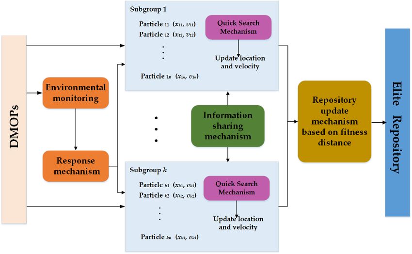
Figure11shows
Figure showsthe
thecomposition
compositionofofthe
theDVEPSO/FD
DVEPSO/FD system,
system, which
whichovercomes
overcomesthe the
shortcomingsofofthe
shortcomings theDVEPSO
DVEPSOmethod
methodthat
thatcannot
cannotobtain
obtainaavery
veryaccurate
accuratePOF
POFtracked
trackedafter
after
eachobjective
each objectivechanges.
changes.The
The repository
repository update
update mechanism
mechanism based
based on fitness
on the the fitness distance
distance and
quick searchsearch
and quick mechanism are designed
mechanism to respond
are designed quickly when
to respond environmental
quickly changes
when environmental
are monitored.
changes are monitored.
Figure1.1.DVEPSO/FD
Figure DVEPSO/FD system.
system.
The
The core
core structures
structures of the DVEPSO/FD
DVEPSO/FDalgorithm algorithmcancan bebe summarized
summarized as as follows:
follows: in-
information sharing mechanism,
formation sharing mechanism, environmental
environmental monitoring
monitoring and response
response mechanism,
mechanism,
quick
quicksearch
searchmechanism,
mechanism, andand repository
repositoryupdate mechanism.
update mechanism. A swarm
A swarmof particles are used
of particles are
to solve
used toDMOPs, and it is
solve DMOPs, divided
and into k subgroups.
it is divided Each particle
into k subgroups. Eachhas its own
particle location
has its own and
lo-
velocity, which are updated in each iteration to obtain pbest and gbest.
cation and velocity, which are updated in each iteration to obtain pbest and gbest . The information
sharing mechanism is adapted to change information between subgroups. The system
The information sharing mechanism is adapted to change information between sub-
monitors changes in the environment in real time. Once it changes, the response mechanism
groups.
will Thepart
pick out system monitors
of the particleschanges
to makeincorresponding
the environment in real time.
adjustments, and Once it changes,
the quick search
the response
mechanism mechanism
will will
be activated pickfirst
at the outtime.
part ofThethe particlesistoused
repository make to corresponding adjust-
store Pareto solutions
ments, and the quick search mechanism will be activated at the first time. The
and it is updated based on fitness distance to obtain an elite repository. The gbest is picked repository
is used
up from to
thestore
elite Pareto solutions
repository andguide
to better it is updated based on fitness distance to obtain an
the particles.
Because the quality of the repository update mechanism largely determines whether
the algorithm can filter out the good nondominant solutions, which will affect the accuracy
of the POF found by the algorithm, an innovation is first made in the repository update
mechanism. The repository update mechanism based on fitness distance is generally based
on the crowding distance, which may delete the better solution, and is not conducive to the
diversity of MOPSO. While the fitness distance is defined and introduced in DVEPSO/FD
to streamline the repository, calculate the average of the distance between the nondominant
solutions with respect to each fitness function, use its average characteristics to streamline
the repository more than once, and eliminate nondominant solutions with invalid or poor
performance. It could be more effective at guiding the selection of the global optimal
solution, thus achieving a better choice of nondominant solutions and maintaining a more
efficient repository.Mathematics 2022, 10, 1587 5 of 13
In addition, in order to improve the efficiency of the algorithm and quickly find the
POF, this paper proposed the addition of a quick search mechanism, that is, dynamically ad-
justing the flight parameters before and after the first change of the environment. Compared
with the DVEPSO method, the repository update mechanism based on fitness distance
could improve the distribution of nondominant solutions, and the quick search mechanism
could adjust dynamically to improve the search speed.
3.2. Module Design
3.2.1. Repository Update Mechanism Based on Fitness Distance
In the past, the repository update mechanism was usually based on crowding distance,
and the nondominant solution beyond the repository size was eliminated directly by
calculating the crowding distance, while the fitness distance was used in DVEPSO/FD to
streamline the repository. The definitions of the crowding distance and fitness distance are
as follows.
Definition 1 ([25]). Crowding distance is defined in Equation (4). Suppose there are a total of m
sub-objectives, and the initial crowding distance of all individuals is I (i )d = 0.
m
Li = ∑( f i+1,k − f i−1,k ) (4)
k =1
where Li is the crowing distance of particle i and m is the number of fitness functions, where the
fitness function is the specific function model of the each objective optimization problem. f i,k is the
k-th fitness function value of particle i.
Definition 2. The definition and equation of fitness distance is shown in Equation (5).
( S ( i + 1) m − S ( i − 1) m )
S (i ) f d m = (5)
f m max − f m min
where S(i ) f d m is the fitness distance of the individual i relative to the objective m, and S(i )m is the
fitness function value of the individual i relative to the objective m. It is important to point out that
if there are M objectives, then each particle has and totally has M fitness distances.
Figure 2 shows a schematic diagram of the repository update mechanism based on
fitness distance. The optimization problem could be divided into several independent fit-
ness functions. For each fitness function, each particle can calculate a corresponding fitness
distance. The fitness distance of the nondominant solution is calculated and compared with
the set threshold α F to determine whether the nondominant solution is retained or not. All
of the fitness distances are used to streamline the repository independently. Compared to
the crowding distance, the repository update mechanism based on the crowding distance is
only streamlined once, but the one based on the fitness distance will be streamlined m times
according to the number of fitness functions. The advantage of this design is that it can
retain its optimal solution for each fitness function. Especially in the case of environmental
changes, the response of each objective is different, so the changes of each fitness function
are different. The repository update mechanism based on the crowding distance may miss
the optimal solution, while the proposed method is more conducive to solve dynamic
optimization problems.
After completing all the streamlining actions, the remaining nondominant solutions
form the elite repository. The elite repository also has a certain capacity, so the number of
nondominant solutions in the elite repository should also be limited, and the elimination
rule is also based on crowding distance when out of range.on the crowding distance is only streamlined once, but the one based on the fitness dis-
tance will be streamlined m times according to the number of fitness functions. The ad-
vantage of this design is that it can retain its optimal solution for each fitness function.
Especially in the case of environmental changes, the response of each objective is different,
so the changes of each fitness function are different. The repository update mechanism
Mathematics 2022, 10, 1587 6 of 13
based on the crowding distance may miss the optimal solution, while the proposed
method is more conducive to solve dynamic optimization problems.
Fitness Streamline
Fitness_1
distance_1 Repository
Elite Repository
Fitnesses
Fitness Streamline
Fitness_2
distance_2 Repository
Fitness Streamline
Fitness_m
Distance_m Repository
Figure 2. Schematic
Figure 2. Schematic diagram
diagram of
of repository
repository update
update mechanism
mechanismbased
basedon
onfitness
fitnessdistance.
distance.
3.2.2.After
Quickcompleting
Search Mechanism
all the streamlining actions, the remaining nondominant solutions
formThe the Pareto optimal frontier
elite repository. ofrepository
The elite the dynamic alsoalgorithm alsocapacity,
has a certain changes so according to the
the number of
change in the objective function. The Pareto optimal frontier of the
nondominant solutions in the elite repository should also be limited, and the elimination first generation is
difficult to find. The Pareto optimal frontier
rule is also based on crowding distance when out of range.of the offspring is changed on the basis of the
previous generation, so it will be easier to find than the first generation.
3.2.2.InQuick
orderSearch
to improve particles’ ability of finding the initial POF quickly in the early stage,
Mechanism
the quick search mechanism is proposed. Iterations before the first time environmental
The Pareto optimal frontier of the dynamic algorithm also changes according to the
change can be named the Quickly Search stage (QS stage); therefore, the value of w, c1 , and
change in the objective function. The Pareto optimal frontier of the first generation is dif-
c2 in the QS stage should be dynamically adjusted. After the QS stage, the next POFs are
ficult to find. The Pareto optimal frontier of the offspring is changed on the basis of the
usually easily found on the basis of the existing data of the previous POF, and this stage
previous generation, so it will be easier to find than the first generation.
can be named the Non-QS stage. The parameters do not need to be dynamically adjusted
In order to improve particles’ ability of finding the initial POF quickly in the early
in the Non-QS stage, which does not contribute much to save the runtime.
stage, the quick search mechanism is proposed. Iterations before the first time environ-
For the adaptive PSO, the values of w and learning factor c1 are required to be large in
mental change can be named the Quickly Search stage (QS stage); therefore, the value of
the early iteration to enhance the search ability of the local optimal value. When close to the
w , cthe
POF, 1 , and
search c2 ability
in theofQSthis
stage should
local optimalbe value
dynamically
shouldadjusted.
be reduced, After the later
so the QS stage,
valuethe
is
next POFs
small. are usually
Conversely, easilyoffound
the value on the
learning basis
factor of required
c2 is the existing data offrom
to change the previous POF,
small to large.
and
In thethis
laterstage can be the
iteration, named the Non-QS
influence stage. The
of the global parameters
optimal value isdo not needtotomake
enhanced be dynam-
more
ically adjusted
particles close to inthe
thePOF.
Non-QSThe stage, which
specific does not
adjustment contribute
equations of much to save
these three the runtime.
parameters in
the QS For stage
the are shownPSO,
adaptive the values of w and learning factor c1 are required to be
in (6)–(8).
large in the early iteration to enhance the search ability of the local optimal value. When
(wmax − wmin )
close to the POF, the searchw(r )ability
= wmaxof −
this local optimal value should be reduced, so the(6)
(1 + exp(5 − 0.07 ∗ r ))
later value is small. Conversely, the value of learning factor c2 is required to change from
where wmax
small to = 0.9,
large. wmin
In the = 0.4,
later and r the
iteration, is the current of
influence number of iterations.
the global optimal value is enhanced
to make more particles close to the POF. The specific adjustment equations of these three
parameters in the QS stage c1 (are 2 − 1/in
r ) =shown (0.98 + exp(10 − 0.1 ∗ r ))
(6)–(8). (7)
c2 (r ) = 1 + 8/(8 + exp((− 13 −
wmax +w min )
1500/r )) (8)
w(r ) = wmax − (6)
3.2.3. Other Structures (1 + exp(5 − 0.07 * r ))
(1) Information sharing mechanism
Each particle has a local optimum and a global optimal to guide its search in the search
space. The local optimum of a particle is its personal best, pbest, which is the best position
where the particle is currently found. When there are no changes in the environment, the
global guide of particles, gbest, is selected from one of the subgroups through a knowledge
sharing mechanism. In this way, the pbest of each population may become gbest, that is, the
information of its own population is transmitted through pbest, and then other populations
are affected by gbest, thereby achieving information sharing between the populations [21].Mathematics 2022, 10, 1587 7 of 13
There are many mechanisms for information sharing, such as the circular loop strategy
and roulette selection. Among them, the circular loop strategy is relatively simple. The
selection method of subgroup s is shown in Equation (9).
k f or j = 1
s= (9)
j − 1 f or j = 2, . . . , k
(2) Environmental monitoring and response mechanism
After each iteration, randomly select some particles as sentinel particles, and evaluate
the environment before the start of the next iteration. If the differences in the fitness
values of the sentinel particles between current and previous are all greater than a certain
value, the environment is considered changed. If a change in the environment is detected,
the particles of the corresponding subgroup are reinitialized at a certain ratio, which is
usually 30%.
3.3. The Pseudo-Code of the Algorithm
The repository update mechanism based on fitness distance possesses the elite reposi-
tory to improve the distribution of nondominant solutions, and the quick search mechanism
adjusts the flight parameters dynamically, so the DVEPSO/FD responds quickly when
environmental changes are monitored. The pseudo-code of the DVEPSO/FD is shown in
Table 1.
Table 1. The pseudo-code of the DVEPSO/FD method.
Pseudo-Code
1. Randomly initialize each particle ( xki , vki ) in the swarm and divide the swarm into
K subgroups, set w0 , c10 , c20 , and clear the repository Re
2. For R from 1 to N, iterating
Randomly select some particles, calculate the fitness f m r (x )
i
r ( x ) − f r −1 ( x ) < α
If f m i m i T
(a) Using vriD +1
= wvriD + c1 r1 pbestri − xiD r r , x r +1 = x r + vr +1 to
+ c2 r2 gbestr − xiD
iD iD iD
update the position and velocity
(b) Determine pbestri by non-dominant relationship, gbestr from subgroup based on
information sharing mechanism
Else
(a) Initiate response mechanism, randomly pick out 30% particles of corresponding
subgroup, initialize the positons and velocities of these particles.
(b) Initiate quick search mechanism, update the position and velocity of the rest particles
wmax −wmin
using w(r ) = wmax − 1+exp (5−0.07∗r )
, c1 (r ) = 2 − 1/(0.98 + exp(10 − 0.1r )),
c2 (r ) = 1 + 8/(8 + exp(−13 + 1500/r )) instead of fixed parameters
(c) Determine pbestri by non − dominant relationship, gbestr from elite repository
End if
S ( i +1) − S ( i −1)
Calculate all the fitness distances S(i )m
fd =
m
f mmax − f mmin
m
,
steamline the repository to form elite repository and update the ReIf Re out of range
Limited elite repository based on crowding distance
End if
End for
4. Experiments and Results
4.1. Standard Benchmarks
The changes based on the POF and Pareto optimal solutions (POSs) [26] can be
classified as four categories. The dynamic multi-objective optimization standard test
problems are mainly FDA [27] (FDA5-iso [28]) series and nonlinear-related DMOP [29]
series. The specific classification [8] and their correspondences with the test functions are
shown in Table 2, and the formulas are defined in Table 3.Mathematics 2022, 10, 1587 8 of 13
Table 2. Classification of standard benchmarks.
POS
POF
No Change Change
Type IV Type I
No change
Problem changes FDA1; FDA4
Type III Type II
Change
FDA2; DMOP1 FDA3; FDA5; DMOP2
Table 3. The formula definition of standard benchmarks.
Benchmarks Definition Benchmarks Definition
f 1 ( X I ) = x1 f 1 ( X I ) = x1
f2 (X I I ) = g · h f2 (X I I ) = g · h
g( X I I ) = 1 + ∑q m
i =2 ( xi − G ( t ))
2
g( X I I ) = 1 + ∑im∈X I I ( xi )2
FDA1 1 f FDA2 H (t)+∑ x ∈ X ( xi − H (t))2
h( f 1 , g) = 1 − g
f
h( X I I I , f 1 , g) = 1 − ( g1 ) i III
G (t) =j sink(0.5π · t) H (t) =j 0.75 k + 0.7 · sin(0.5π · t)
t = n1t ττt t = n1t ττt
where| X I I | = 9, X I ∈ [0, 1], X I I ∈ [−1, 1] where| X I I | = | X I I I | = 15, X I ∈ [0, 1], X I I , X I I I ∈ [0, 1]
f 1 ( X I ) = ∑ xi ∈ X I x i F ( t ) f 1 ( X ) = (1 + g( X I I ))∏iM −1 i xπ
=1 cos( 2 )
f2 (X I I ) = g · h M −1 xπ x π
f k ( X ) = (1 + g( X I I ))∏i=1 (cos( i2 )) sin( M−2k+1 )
g( X I I ) = 1 + G (t) + ∑ xi ∈X I I ( xi − G (t))2 M −1 x1 π
f M ( X ) = (1 + g( X I I ))∏i=1 sin( 2 )
q
f1
FDA3
h( f 1 , g) = 1 − g
FDA 4 g( X I I ) = ∑ xi ∈X I I ( xi − G (t))2
G (t) = |sin(0.5π · t)| G (t) =j |sink (0.5π · t)|
F (t) =j102ksin(0.5π ·t) t = n1t ττt
t = n1t ττt where X ∈ [0, 1]
where| X I | = 5, | X I I | = 25, X I ∈ [0, 1], X I I ∈ [−1, 1]
−1 yi π −1 yπ
f 1 ( X ) = (1 + g( X I I ))∏iM =1 cos( 2 ) f 1 ( X ) = (1 + g( X I I ))∏iM =1 cos( 2 )
i
−1 yi π y M − k +1 π −1 yi π y M − k +1 π
f k ( X ) = (1 + g( X I I ))∏iM =1 ( cos ( 2 )) sin( 2 ) f k ( X ) = (1 + g( X I I ))∏iM=1 ( cos ( 2 )) sin( 2 )
M −1 y1 π M −1 y1 π
f M ( X ) = (1 + g( X I I ))∏i=1 sin( 2 ) f M ( X ) = (1 + g( X I I ))∏i=1 sin( 2 )
g( X I I ) = G (t) + ∑ xi ∈X I I (yi − G (t))2 g( X I I ) = ∑ xi ∈X I I (yi − G (t))2
FDA5 yi = xi F (t) FDA5-iso yi = xi F (t)
G (t) = |sin(0.5π · t)| G (t) = |sin(0.5π · t)|
F (t) =j1 +k 100 sin4 (0.5π · t) F (t) =j1 +k 100 sin4 (0.5π · t)
t = n1t ττt t = n1t ττt
where X ∈ [0, 1] where X ∈ [0, 1], X I I = ( x M , . . . , xn )
f 1 ( x1 ) = x1 f 1 ( x1 ) = x1
f 2 ( x2 , . . . , x m ) = g · h f 2 ( x2 , . . . , x m ) = g · h
g( x2 , . . . , xm ) = 1 + 9 · ∑im=2 xi 2 g( x2 , . . . , xm ) = 1 + ∑im=2 ( xi − G (t))2
DMOP1 DMOP2 f H (t)
H (t)
f
h( f 1 , g) = 1 − ( g1 ) h( f 1 , g) = 1 − ( g1 )
H (t) = 0.75 · sin(0.5π · t) + 1.25 H (t) = 0.75 · sin(0.5π · t) + 1.25
where m = 10, xi ∈ [0, 1] G (t) = sin(0.5π · t)
where m = 10, xi ∈ [0, 1]
4.2. Performance Metrics
Weicker proposed that it is necessary to consider the metrics he describes when analyz-
ing and comparing algorithms for dynamic problems. They are accuracy and stability [30].
(1) Accuracy
The accuracy measures how close the best solution is found to the actual one. It usually
takes a value between 0 and 1, where 1 is the best precision value. The specific definition is
shown in Equation (10).
F (best EA (t)) − minF (t)
accurracy F,EA (t) = (10)
maxF (t) − minF (t)
where best EA (t) is the best solution found in the population at time t, the maximum and
minimum fitness values in the search space are represented by maxF (t) and minF (t), and
F is the fitness function of the objective problem.Mathematics 2022, 10, 1587 9 of 13
(2) Stability
The stability measures the stability of dynamic algorithms, which would be called
stable algorithms when they do not seriously affect the accuracy of optimization. Stability
is an important issue for optimization in dynamic environments. Its value ranges from 0
to 1, where a value close to 0 indicates higher stability. The definition of stability is as in
Equation (11).
stabF,EA (t) = max{0, accurracy F,EA (t) − accurracy F,EA (t − 1)} (11)
4.3. Parameters’ Settings
There are six subgroups and each swarm has 50 particles. The size of the repository
is set to 100, and 30% of the particles are reinitialized after an environmental change is
detected. In addition, other parameters are shown in Table 4, where τt is the environment
change frequency.
Table 4. Parameters’ settings.
Parameters nt τt w0 c10 c20 R
15 0.72 1.49 1.49
Values 100 1000
(FDA2: 2.5) (Non-QS stage) (Non-QS stage) (Non-QS stage)
4.4. Experiments
The experiments are carried out on the standard benchmarks that have been mentioned
in Table 3 separately. The specific results of each test function are shown in Figure 3a–n.
There are two pictures shown in each test function. The first one is the Pareto front found
by the basic algorithm (DVEPSO), and the second one is the Pareto front found by the
proposed algorithm (DEVPSO/FD). Different colors in the pictures represent different
changed POFs.
Table 5 records the performance metrics of the experiments above, which are accuracy,
stability, and their respective runtimes of DVEPSO and DVEPSO/FD. In Table 5, Mean is
the mean, Std is the standard deviation, and Best is the best value.
Table 5. The accuracy and stability metrics on benchmarks.
Accuracy Stability Runtime
Benchmarks
DVEPSO DVEPSO/FD DVEPSO DVEPSO/FD DVEPSO DVEPSO/FD
Mean 0.4292 0.4236 0.0223 0.0209
FDA1 Std 0.0015 0.0004 0.0012 0.0007 111.1841 222.6885
Best 0.4308 0.4239 0.0237 0.0213
Mean 0.5621 0.5712 0.0399 0.0323
FDA2 Std 0.0088 0.0065 0.0010 0.0021 139.2537 141.3722
Best 0.5722 0.5741 0.0411 0.0338
Mean 0.6846 0.6849 0.0412 0.0290
FDA3 Std 0.0012 0.0043 0.0054 0.0009 119.9075 125.3159
Best 0.6859 0.6916 0.0472 0.0297
Mean 0.2423 0.2482 0.0284 0.0297
FDA4 Std 0.0012 0.0023 0.0008 0.0013 161.0242 675.8527
Best 0.2432 0.2499 0.0293 0.0310
Mean 0.2269 0.2342 0.0256 0.0249
FDA5 Std 0.0015 0.0023 0.0010 0.0003 168.8640 492.0685
Best 0.2284 0.2368 0.0263 0.0251
Mean 0.6194 0.6228 0.0204 0.0165
DMOP1 Std 0.0054 0.0030 0.0020 0.0046 159.8208 1213.6000
Best 0.6255 0.6296 0.0227 0.0218
Mean 0.5680 0.5691 0.0136 0.0139
DMOP2 Std 0.0005 0.0011 0.0003 0.0006 118.3666 163.2108
Best 0.5683 0.5694 0.0139 0.0146Mathematics 2022, 10, x1587
Mathematics FOR PEER REVIEW 1110ofof 15
13
(a) (b) (c) (d)
(e) (f) (g) (h)
(i) (j) (k) (l)
(m) (n)
Figure
Figure 3.
3. Simulation
Simulation results
results on
on benchmarks:
benchmarks: (a)
(a) POF
POF ofof DVEPSO on FDA1,
DVEPSO on FDA1, (b)
(b) POF
POF of
of DEVPSO/FD
DEVPSO/FD
on FDA1, (c) POF of DVEPSO on FDA2, (d) POF of DEVPSO/FD on FDA2, (e) POF of DVEPSO on
on FDA1, (c) POF of DVEPSO on FDA2, (d) POF of DEVPSO/FD on FDA2, (e) POF of DVEPSO on
FDA3, (f) POF of DEVPSO/FD on FDA3, (g) POF of DVEPSO on FDA4, (h) POF of DEVPSO/FD on
FDA3, (f) POF of DEVPSO/FD on FDA3, (g) POF of DVEPSO on FDA4, (h) POF of DEVPSO/FD
FDA4, (i) POF of DVEPSO on FDA5, (j) POF of DEVPSO/FD on FDA5, (k) POF of DVEPSO on
on FDA4,(l)(i)POF
DMOP1, POFofofDEVPSO/FD
DVEPSO on on FDA5, (j) POF
DMOP1, (m)ofPOF
DEVPSO/FD
of DVEPSOonon
FDA5, (k) POF
DMOP2, and of
(n)DVEPSO
POF of
on DMOP1, (l)
DEVPSO/FD onPOF of DEVPSO/FD on DMOP1, (m) POF of DVEPSO on DMOP2, and (n) POF of
DMOP2.
DEVPSO/FD on DMOP2.
Table 5 records the performance metrics of the experiments above, which are accu-
4.5. Results
racy, stability, and their respective runtimes of DVEPSO and DVEPSO/FD. In Table 5,
MeanFrom
is thethe POFStd
mean, figures
is theofstandard
FDA1~FDA5 and DMOP1~DMOP2,
deviation, and Best is the bestitvalue.
can be seen that the
algorithm that used the fitness distance to streamline the repository, that is, DVEPSO/FD,
has clearer POFs and is more accurate than DVEPSO. FD2, FD3, FD5, DMOP1, and DMOP1
are all classified as the POF changed. When the POF is dynamically changing, it can be seen
from the figures that the lines between those changed POFs are also clearer, which indicates
that DVEPSO/FD can find better solutions. In particular, the POF of the DVEPSO/FD can
converge faster in the early stage of the optimization objective environment change, which
indicates that the quick search mechanism proposed by the algorithm has also played an
important role.Mathematics 2022, 10, 1587 11 of 13
Accuracy represents the precision of the solutions, and the closer its value to 1, the
higher the accuracy. It can be seen from Table 5 that the accuracy of FDA4 with the POS
changed obtained by DVEPSO/FD is 2.43% higher than that of DVEPSO; the accuracy
of FDA3, FDA5, and DMOP2 with both the POF and POS changed can be improved by
3.22%; and the accuracy of FDA2 and DMOP1 with the POF changed can be improved
by 1.62%, while the accuracy of FDA1 obtained by DVEPSO/FD is lower than that of
DVEPSO. As FDA1 has two objective functions and no change in the POF, DVEPSO/FD
does not show its advantages. Although the accuracy data of FDA1 are slightly lower, a
more accurate POF and accurate solutions can still be found by DVEPSO/FD. On the other
hand, DVEPSO/FD shows good performance on the complex problems, especially when
the POF and POS both change on three objectives.
Stability represents the solid state of the algorithm, and the closer its value to 0, the
better the stability. As can be seen from Table 5, the stability values of DVEPSO are all
between 0.01 and 0.05, which are still very close to 0. It indicates that the stability is very
good under such a condition. Similarly, the stability values of DVEPSO/FD are all between
0.01 and 0.04, which are even better than DVEPSO, improved at most by 19.12%. The
results of the stability index show that DVEPSO/FD does not destabilize the algorithm and
maintain the original high stability.
As for the runtime, due to the dynamic adjustment of the flight parameters of the
particles, the particles can quickly find the POF of the first generation, thereby saving a
certain time. However, as the repository update mechanism using the fitness distance
has more steps than the crowding distance condition, the running time of the overall
algorithm of DVEPSO/FD is longer than that of DVEPSO. It can be seen from Table 5 that,
for dual objective functions and slightly simpler nonlinear problems, such as FDA1, FDA2,
FDA3, and DMOP1, the runtimes of DVEPSO/FD do not increase by much, while for three
objective functions and complex nonlinear problems, such as FDA4, FDA5, and DMOP2,
the runtimes increase by a factor of three or more. In addition to extremely complex
problems, the test functions selected in this paper can basically represent the complexity of
dynamic multi-objective optimization problems. Therefore, in order to obtain a better POF,
although the running time is increased, it is still within an acceptable range.
In summary, DVEPSO/FD achieves a higher accuracy and stability with the POF
dynamically changing, which shows a good dynamic change adaptability and solving the
set ability of the dynamic multi-objective optimization problem.
5. Conclusions
In this paper, a quick search dynamic vector-evaluated particle swarm optimization
algorithm based on fitness distance (DVEPSO/FD) is proposed. Taking the DVEPSO
method as a foundation, the repository update mechanism using the fitness distance and
quick search mechanism are designed aiming for a good dynamic change adaptability
and solving set ability of the dynamic multi-objective optimization problem. The fitness
distance is used to streamline the repository to achieve better optimal solutions, and the
flight parameters of the particles are adjusted dynamically to improve the search speed.
Both from the figures generated by the experiments of test functions and the values of
performance indexes, the DVEPSO/FD has a better accuracy of the POF than the basic
DVEPSO, obtains a better POS, and maintains the same strong stability.
From the perspective of the overall algorithm structure, the update mechanism of the
repository has a great influence on whether the optimal value could be found closer to the
real POF or not. DVEPSO/FD verifies this more clearly by improving this mechanism. Of
course, other structures of the algorithm are also important, such as the environmental
monitoring and response mechanism and information sharing mechanism. They will
influence whether the algorithm can respond quickly and accurately to changes in the
environment and correctly grasp the general direction of all population evolutions. This is
also the direction of the author’s future research.Mathematics 2022, 10, 1587 12 of 13
Author Contributions: Conceptualization, S.W. and D.M.; methodology, S.W. and M.W.; software,
D.M.; validation, S.W. and D.M.; formal analysis, S.W. and M.W.; investigation, S.W. and D.M.;
resources, S.W. and M.W.; data curation, D.M.; writing—original draft preparation, S.W. and D.M.;
writing—review and editing, S.W. and M.W.; visualization, D.M.; supervision, M.W.; project adminis-
tration, S.W.; funding acquisition, S.W. All authors have read and agreed to the published version of
the manuscript.
Funding: This research was supported by the National Natural Science Foundation of China with
grant No. 62003350, and the Fundamental Research Funds for the Central Universities of China with
grant No.2022YQJD16.
Data Availability Statement: The data presented in this study are available upon reasonable request
from the corresponding author.
Conflicts of Interest: The authors declare no conflict of interest.
References
1. Coello, A.C.; Lechuga, M.S. MOPSO: A Proposal for Multiple Objective Particle Swarm. In Proceedings of the 2002 Congress on
Evolutionary Computation, Honolulu, HI, USA, 12–17 May 2002; Volume 2, pp. 1051–1056.
2. Coello, C.A.C.; Pulido, G.T.; Lechuga, M.S. Handling Multiple Objectives with Particle Swarm Optimization. IEEE Trans. Evol.
Comput. 2004, 8, 256–279. [CrossRef]
3. Yao, S.; Dong, Z.; Wang, X.; Ren, L. A Multiobjective multifactorial optimization algorithm based on decomposition and dynamic
resource allocation strategy. Inf. Sci. 2020, 511, 18–35. [CrossRef]
4. Helbig, M.; Engelbrecht, A.P. Population-based metaheuristics for continuous boundary-constrained dynamic multi-objective
optimisation problems. Swarm Evol. Comput. 2014, 14, 31–47. [CrossRef]
5. Jiang, M.; Member, S.; Huang, Z.; Qiu, L.; Huang, W.; Yen, G.G. Transfer Learning-Based Dynamic Multiobjective Optimization
Algorithms. IEEE Trans. Evol. Comput. 2018, 22, 501–514. [CrossRef]
6. Helbig, M.; Engelbrecht, A. Dynamic Vector-evaluated PSO with Guaranteed Convergence in the Sub-swarms. In Proceedings of
the 2015 IEEE Symposium Series on Computational Intelligence, Cape Town, South Africa, 7–10 December 2015; pp. 1286–1293.
7. Helbig, M.; Engelbrecht, A.P. Using Headless Chicken Crossover for Local Guide Selection When Solving Dynamic Multiobjetive
Optimization. In Advances in Nature and Biologically Inspired Computing; Springer: Cham, Switzerland, 2016; p. 419.
8. Ou, J.; Zheng, J.; Ruan, G.; Hu, Y.; Zou, J.; Li, M. A pareto-based evolutionary algorithm using decomposition and truncation for
dynamic multi-objective optimization. Appl. Soft Comput. J. 2019, 85, 105673. [CrossRef]
9. Goldberg, D.E.; Smith, R.E. Nonstationary function optimization using genetic algorithm with dominance and diploidy. In
Proceedings of the Second International Conference on Genetic Algorithms and Their Application, Cambridge, MA, USA, 28–31
July 1987; Grefensette, J.J., Ed.; Lawrence Erlbaum Associates Inc.: Mahwah, NJ, USA, 1987; pp. 59–68.
10. Ortega, J.; Toro, F.; De Mario, C. A single front genetic algorithm for parallel multi-objective optimization in dynamic environments.
Neurocomputing 2009, 72, 3570–3579.
11. Guntsch, M.; Middendorf, M.; Schmeck, H. An ant colony optimization approach to dynamic TSP. In Proceedings of the Genetic
and Evolutionary Computation Conference, San Francisco, CA, USA, 7–11 July 2001; Morgan Kaufmann: Burlington, MA, USA,
2001; pp. 860–867.
12. Trojanowski, K. Immune-based algorithms for dynamic optimization. Inf. Sci. J. 2009, 179, 1495–1515. [CrossRef]
13. Zhang, Z. Multiobjective optimization immune algorithm in dynamic environments and its application to greenhouse control.
Appl. Soft Comput. 2008, 8, 959–971. [CrossRef]
14. Pelta, D.; Cruz, C.; Verdegay, J.L. Simple control rules in a cooperative system for dynamic optimisation problems. Int. J. Gen.
Syst. 2009, 38, 701–717. [CrossRef]
15. Urade, H.S.; Patel, R. Dynamic Particle Swarm Optimization to Solve Multi-objective Optimization Problem. Procedia Technol.
2012, 6, 283–290. [CrossRef]
16. Optimization, D.M.; Zhou, A.; Jin, Y.; Member, S.; Zhang, Q.; Member, S. A Population Prediction Strategy for Evolutionary. IEEE
Trans. Cybern. 2014, 44, 40–53.
17. Azzouz, R.; Bechikh, S.; Ben, L. A dynamic multi-objective evolutionary algorithm using a change severity-based adaptive
population management strategy. Soft Comput. 2017, 21, 885–906. [CrossRef]
18. Deb, K.; Rao, N.U.B.; Karthik, S. Dynamic multi-objective optimization and decision-making using modied NSGA-II: A case
study on hydro-thermal power scheduling. In Proceedings of the International Conference on Evolutionary Multi-criterion
Optimization, Matsushima, Japan, 5–8 March 2007; pp. 803–817.
19. Branke, J.; Blackwell, T. Multiswarms, exclusion, and anti-convergence in dynamic environments. IEEE Trans. Evol. Comput. 2006,
10, 459–472.
20. Janson, S.; Middendorf, M. A hierarchical particle swarm optimizer for noisy and dynamic environments. Genet. Program.
Evolvable Mach. 2006, 7, 329–354. [CrossRef]Mathematics 2022, 10, 1587 13 of 13
21. Greeff, M.; Engelbrecht, A.P. Solving dynamic multi-objective problems with vector evaluated particle swarm optimisation. In
Proceedings of the 2008 IEEE Congress on Evolutionary Computation (IEEE World Congress on Computational Intelligence),
Hong Kong, China, 1–6 June 2008; pp. 2917–2924.
22. Parsopoulos, K.E.; Vrahatis, M.N. Recent approaches to global optimization problems through Particle Swarm Optimization. Nat.
Comput. 2002, 1, 235–306. [CrossRef]
23. Helbig, M.; Engelbrecht, A.P. Analyses of Guide Update Approaches for Vector Evaluated Particle Swarm Optimisation on
Dynamic Multi-Objective Optimisation Problems. In Proceedings of the 2012 IEEE Congress on Evolutionary Computation,
Brisbane, QLD, Australia, 10–15 June 2012.
24. Schaffer, J. Multiple objective optimization with vector evaluated genetic algorithms. In Proceedings of the 1st Intenational
Conference on Genetic Algorithms, Sheffield, UK, 12–14 September 1985; pp. 93–100.
25. Peng, G.; Fang, Y.W.; Peng, W.S.; Chai, D.; Xu, Y. Multi-objective particle optimization algorithm based on sharing-learning and
dynamic crowding distance. Optik 2016, 127, 5013–5020. [CrossRef]
26. Saremi, S.; Mirjalili, S.; Lewis, A.; Liew, A.W.C.; Dong, J.S. Enhanced multi-objective particle swarm optimisation for estimating
hand postures. Knowl.-Based Syst. 2018, 158, 175–195. [CrossRef]
27. Farina, M.; Deb, K.; Amato, P. Dynamic Multiobjective Optimization Problems: Test Cases, Approximations, and Applications.
IEEE Trans. Evol. Comput. 2004, 8, 425–442. [CrossRef]
28. Helbig, M.; Engelbrecht, A.P. Benchmarks for Dynamic Multi-objective Optimisation. In Proceedings of the 2013 IEEE Symposium
on Computational Intelligence in Dynamic and Uncertain Environments (CIDUE), Singapore, 16–19 April 2013; pp. 84–91.
29. Goh, C.; Tan, K.C. A Competitive-Cooperative Coevolutionary Paradigm for Dynamic Multiobjective Optimization. IEEE Trans.
Evol. Comput. 2009, 13, 103–127.
30. Weicker, K. Performance Measures for Dynamic Environments. In International Conference on Parallel Problem Solving from Nature;
Springer: Berlin/Heidelberg, Germany, 2002; pp. 64–76.You can also read