(A)SYNCHRONOUS HOUSING MARKETS OF GLOBAL CITIES - MUNICH PERSONAL REPEC ARCHIVE - MUNICH ...
←
→
Page content transcription
If your browser does not render page correctly, please read the page content below
Munich Personal RePEc Archive

(A)Synchronous Housing Markets of
Global Cities

Bhatt, Vipul and Kishor, N. Kundan

14 April 2021

Online at https://mpra.ub.uni-muenchen.de/107175/
MPRA Paper No. 107175, posted 15 Apr 2021 09:30 UTC
(A)Synchronous Housing Markets of Global Cities

                                 Vipul Bhatt∗                N. Kundan Kishor†
                                                  April 14, 2021

                                                      Abstract

      In this paper we examine house price synchronization in 15 global cities using real house price data from
      1995:Q1-2020:Q2. We find that although there is evidence for bilateral positive phase synchronization,
      there is no evidence for an integrated global housing market for our sample of cities. Using a hierarchical
      clustering approach, we identify three clusters of cities with similar housing price cycles that are not
      solely determined by geographic proximity. We interpret this finding as suggestive of a rather segmented
      housing market for the global cities in our sample. Using a dynamic factor model with time-varying
      stochastic volatility we decompose a city’s real housing price growth into a global component, a cluster-
      based component, and an idiosyncratic component. For most cities in our sample, the global component
      plays a minor role, whereas the cluster-based factor explains a large fraction of the observed variation in
      real house price growth with its contribution peaking during the Great Recession of 2007-09.
      JEL Classifications: C38, E32, F36, F44, R30
      Keywords: Global Housing Market, House Price Synchronization, Cluster Analysis, Dynamic Factor
      Model

   ∗ 421, Bluestone Dr., MSC 0204, Department of Economics, James Madison University, Harrisonburg, VA 22807. Email:

bhattvx@jmu.edu.
   † Department of Economics, University of Wisconsin-Milwaukee, Bolton Hall, Milwaukee, WI 53201.            Email:
Kishor@uwm.edu.
1 Introduction
The central role played by the housing market in the 2007-09 financial crisis spurred substantial interest in
housing market dynamics and its implications for the macroeconomy. One feature of the housing market
that has particularly drawn attention is intra- and inter-country synchronization of housing prices.1 This
research has been motivated by the observation that the housing market across many countries witnessed
a rapid boom prior to 2008 and then experienced a sharp decline. The interest in synchronization has
also been fueled by an increasingly globalized economy and greater financial sector openness especially in
the advanced economies. The co-movement of housing prices is of interest to various stakeholders. For
example, for investors looking for high yield opportunities and portfolio diversification, a high degree of
synchronization in housing prices will reduce the diversification benefits of real estate assets in their portfolio.
For policymakers, given the importance of housing price shocks as a leading indicator of financial sector
instability, a high degree of synchronization would imply a greater susceptibility to external shocks. It will
also require a careful assessment of the efficacy of macroeconomic prudential policies in taming housing price
bubbles.2
There is large literature in recent years that has focused on examining housing market synchronization
in terms of co-movement of housing prices across different countries. However, there is no consensus on
the degree of synchronization. For example, several recent contributions have documented substantial and
increasing level of house price synchronization across advanced economies (see, Otrok and Terrones (2005),
Hirata et al. (2012), Katagiri (2018) and Kallberg et al. (2014)). In contrast, Miles (2017) and Tsai (2018)
find a relative lack of such synchronization in international housing markets. Further, there is evidence that
even within a country the housing market may not be fully integrated (see, Miles (2015) and Hernández-
Murillo et al. (2017) for the U.S., Hiebert and Roma (2010) for Europe and the U.S., Klarl (2018) for
Netherlands and Funke et al. (2018) for the U.K. housing market.).
It is reasonable to argue that global financial conditions and investor behavior is more likely to be prevalent
in housing markets of major international cities that in turn drives the linkages observed in national housing
markets. In fact, there has been great deal of media attention on the degree of integration in housing prices of
the so called ”Superstar Cities” or ”Global Cities” that serve as hubs for global financial and trade linkages.3
1 In
our discussion we use housing market synchronization and house price synchronization interchangeably.
2 There are various channels through which housing markets may synchronize across national borders. For instance if a group
of countries share strong trade linkages and exhibit synchronization in real economic activity then it is reasonable to expect
a high degree of synchronization in the housing market as well. Similarly, a higher degree of synchronization in interest rates
across different countries may induce similar cycles in housing markets.
3 Gyourko et al. (2013) use ”Superstar Cities” term for major cities in the U.S. However, many business news platforms
commonly use labels such as ”global cities” or ”superstar cities” to include major cities across the globe. For example, see
1These cities also tend to have excellent physical and institutional infrastructure that can increase demand
for housing in these cities. The Economist magazine provides an interactive guide on the housing prices of
major international cities and offer regular commentary on the level of synchronization in some of the most
desirable cities across the globe.4 UBS Group provides a Global Real Estate Bubble Index where they track
housing markets of 25 global cities.5 This index is often used in the media to speculate on the formation
of housing price bubbles in the globalized housing market.6 One common theme in such discussions is the
potential for housing price bubbles in these cities which is often attributed to an influx of funds from foreign
investors seeking high yield investment opportunities. In many cases governments have imposed outright
bans on foreign ownership of real estate or have used taxes to tame housing prices in their major cities. For
example, in recent years Canada and Australia have used taxes and other restrictions to limit flow of funds
from China in the housing market of their major cities such as Vancouver and Sydney.7
Although the housing market in the global cities have drawn attention worldwide through media spe-
cializing in business news, the academic literature on the evolution and synchronization is relatively scarce
because of limited availability of time-series data.There are two exceptions: International Monetary Fund
(2018) and Katagiri (2018). According to the 2018 Global Financial Stability Report by International Mon-
etary Fund (IMF) the increase in synchronization for the 2013-2017 period is more pronounced across major
cities than across countries, especially in the case of advanced economies International Monetary Fund (2018).
Katagiri (2018) focuses on city-level variations within the economy. Both of these studies are constrained
by a short sample period that was particularly affected by the after effects of the housing bust that took
place during the financial crisis.8 Our paper attempts to bridge this gap in the literature by using quarterly
data from 1995:Q1 through 2020:Q2 on 15 global cities.9 This paper seeks to answer the following research
questions. First, are housing markets in major international cities highly integrated, or do we find evidence
for a ”cluster” of cities that share housing price dynamics? Answers to this question will inform us whether
an integrated global housing market is a correct characterization. Following the literature on business cycles,
https://www.mckinsey.com/featured-insights/innovation-and-growth/superstars-the-dynamics-of-firms-sectors-an
d-cities-leading-the-global-economy.
4 See, https://www.economist.com/graphic-detail/2016/03/31/global-house-prices. The discussion on global city
housing price can be found at: https://www.economist.com/graphic-detail/2019/03/11/global-cities-house-price-index
5 For details on this index see https://www.ubs.com/global/en/wealth-management/chief-investment-office/life-goa
ls/real-estate/2020/global-real-estate-bubble-index.html.
6 A recent example can be found at: https://www.cnbc.com/2020/09/30/these-cities-are-at-risk-of-a-housing-bubb
le-as-home-prices-inflate-worldwide.html
7 https://www.wsj.com/articles/western-cities-want-to-slow-flood-of-chinese-home-buying-nothing-works-1528
294587
8 Our methodology also allows for endogenous treatment of clusters and more general treatment of time-varying volatility.
See details in Section 4.
9 Our sample of cities include Amsterdam, Chicago, Copenhagen, Hong Kong, London, New York City, Oslo, Paris, San
Francisco, Singapore, Stockholm, Sydney, Tokyo, Toronto, and Vancouver.
2we compute a pairwise phase synchronization measure that captures whether the housing price expansions
(contractions) of two cities are synchronized. To provide suggestive evidence on how similar housing price
dynamics of cities in our sample are, we employ a hierarchical cluster approach to identify the clusters of
cities that exhibit similar house price dynamics. An integrated housing market would imply that there is a
large cluster that encompasses all cities whereas a segmented housing market would imply multiple clusters
of cities with similar housing price dynamics. Our second research question pertains to the evolution of
the synchronization of city-level house prices over time. We use a dynamic factor model with time-varying
stochastic volatility to estimate the contribution of a global common factor affecting all cities in our sample,
a cluster-level factor that only affects cities in a given cluster, and an idiosyncratic city-level factor. These
clusters are determined by the hierarchical cluster approach and our model allows us to estimate time varying
contributions of these factors.
There are several findings of interest. First, we find evidence for significant pairwise synchronization in
our sample of cities with several city-pairs likely to be in the same phase of the housing price cycle at the same
time.10 We also find that this finding is true for several city-pairs located in different continents. For example,
Toronto is significantly synchronized with many cities in Europe and Sydney is positively synchronized
with San Francisco. These findings indicate that geography is not the primary reason for housing price
synchronization for city-pairs in our sample. Second, our cluster analysis reveals a rather segmented global
housing market with three unique clusters of cities.The first cluster has Vancouver and three Asian cities:
Hong Kong, Singapore and Tokyo. The second cluster has 4 cities: Amsterdam, Chicago, New York City
and Oslo. The third cluster has seven cities: Copenhagen, London, Paris, San Francisco, Stockholm, Sydney
and Toronto. Again, we find that geography does not seem to be the only factor driving synchronization
in house price cycles in our sample.11 The results from our dynamic factor model indicate that the global
factor does not contribute significantly to housing price real growth for most cities in our sample. In contrast
for many cities the cluster factor seems to play an important role with its contribution peaking during the
Great Recession of 2008-09. Higher degree of synchronization of the cities within their respective clusters
during the financial crisis seem to suggest state-dependence in housing price synchronization.12
The remainder of the paper is organized as follows: Section 2 discusses the data used in the paper;
10 Phase implies expansion and contraction of housing market in this study.
11 Note that there is some evidence that geography may not be the primary factor driving housing price cycles for the U.S. For
example, Hernández-Murillo et al. (2017) found that different clusters of cities do not necessarily share geographic similarity
and exhibit their own idiosyncratic volatility.
12 Hale (2012) documents state-dependence for banking networks with a decline in the number of bank relationships in the
global banking network during episodes of recessions in the U.S. For the housing market. Claessens et al. (2010, 2012) document
that housing price cycles are highly synchronized and the degree of co-movement is higher during periods of synchronized
recessions.
3Section 3 details the model specification for synchronization and cluster analysis; Section 4 provides a model
framework for a dynamic factor model with stochastic volatility and its results; Section 5 discusses the
empirical results and policy implications ; and Section 6 provides a conclusion.
2 Data
The main variable of interest is the real housing price index. Our sample composition is primarily driven
by our objective to include as many large international cities as allowed by the availability of reasonably
long quarterly time series. Our final sample consists of quarterly data from 1995Q1 through 2020Q2 and
covers 15 cities spanning North America, Europe, Asia, and Australia. We include the following six cities
from Europe: Amsterdam, Copenhagen, London, Paris, Oslo, and Stockholm. Five North American cities
include Chicago, New York City (NYC), San Francisco, Toronto, and Vancouver. Finally, we include three
cities from Asia (Hong Kong, Singapore, and Tokyo) and Sydney from Australia.13 The data is sourced
from national statistical agencies, Bank of International Settlements, and FRED database maintained by
the Federal Reserve Bank of St. Louis. Table A.1 in the appendix A provides a detailed description of the
housing price index for each city in our sample.
Our main variable of interest is the annualized growth rate of real housing price index of city i at time t:
" 4 #
RHP Iit
yit = − 1 · 100 (1)
RHP Iit−1
where RHP Iit denotes real housing price index of city i at time t.14
Table 1 provides descriptive statistics for real housing price growth for each city in our sample. Over
our sample period Copenhagen experienced highest average growth in real housing prices followed by Paris.
Tokyo experienced negative growth. Further, average housing price growth seems to be much higher in
Europe when compared to cities in North America, Asia, and Australia. We also provide data on peak and
trough in housing growth for each city. One interesting finding is that for many cities in our sample the trough
seems to center around the Great Recession spanning 2007 and 2009. In contrast, there is no synchronization
in the peak across these cities. The higher synchronization in trough date is suggestive of state-dependence
in the relationship between housing price growth across cities in our sample. This finding is consistent with
13 Singapore is a city-state and Hong Kong is a metropolitan area that is officially a special administrative region of the
People’s Republic of China.
14 To compute real housing price index of a city we deflate the nominal index by city or metropolitan area level consumer
price index where available. For Amsterdam, Copenhagen, London, Paris, Oslo, and Stockholm we use national consumer price
index data as the city level data was not available for these cities in our sample.
4the literature on banking networks where number of connections decrease during recessions(Hale, 2012) and
greater degree of synchronized housing price cycles during downturns (Claessens et al., 2010, 2012).
3 Synchronization in Housing Prices
In this section we present the econometric methodology used to measure synchronization in housing price
dynamics of 15 cities in our sample. We use the framework of Mink et al. (2012) for business cycle syn-
chronization based on whether positive (negative) output gaps coincide across nations. This approach has
been used for national house price synchronization (Miles, 2017) and credit cycle synchronization(Meller and
Metiu, 2017). The discussion in this section closely follows the regression-based framework used in Meller
and Metiu (2017) to measure and test for the presence of phase synchronization between housing cycles of
pairs of cities in our sample.
3.1 Phase synchronization between city-pairs
One of the recurrent issues in the synchronization literature is how to transform the variable of interest:
should it be the growth rate of the variable or a trend-cycle decomposition based cycle. In order to avoid the
complications associated with model based cycles, we use a model free approach and use annualized growth
rate of housing prices from equation (1). This approach is also consistent with the existing work in the
literature. See for example, Hirata et al. (2012) and Kose et al. (2003), among others. We create a binary
variable to identify whether a city is experiencing positive or negative housing price growth as follows:
yit 1 if housing price growth is positive
Dit = = (2)
|yit |
−1 if housing price growth is negative
We interpret Dit as a measure of the housing market phase that the city i is experiencing at t. Based on
this we define a measure of pairwise phase synchronization, denoted by P Si,j,t between two cities i and j,
as follows:
1 if cities i and j are in the same phase at time t
P Si,j,t = Dit · Djt = (3)
−1 if cities i and j are not in the same phase at time t
5An alternative way to measure synchronicity would have been to look at the Pearson’s correlation coefficient
between housing price growth of pairs of cities. This approach does not require transforming our continuous
data into a binary variable which as noted in this comment amounts to losing information. However, for
our purpose we believe that such a measure is not suitable for the following reason. Depending on their
respective standard deviations, two time series can have a low correlation and yet experience a high degree
of phase synchronization in the following sense: they enter periods of expansions or contractions in their
housing markets roughly at the same time. In this paper we want to measure synchronization between
different phases of house price cycles in our sample of cities. The binary transformation we implement in
equations (2) and (3) is a more appropriate measure for this purpose.15
Following Meller and Metiu (2017) we use the over time average of the above measure to test for phase
synchronization between each pair of cities in our sample. Formally, let ωij = E(P Sijt ) denote the uncon-
ditional mean of phase synchronization between cities i and j. Then our null hypothesis is given by:
H0 : ωij ≤ 0 → no synchronization or negative synchronization (4)
The right-tailed alternative hypothesis is given by:
HA : ωij > 0 → positive synchronization (5)
In order to implement the above test, we estimate the following linear regression model using OLS and
adjust standard errors for possible serial correlation:
P Sijt = ωij + νijt (6)
Table 2 presents the results of pairwise phase synchronization for 15 cities in our sample. We find that
for several city-pairs there is evidence for positive phase synchronization that is both statistically significant
and economically meaningful. First, in our sample, only the US and Canada have more than one city and in
both cases we find strong evidence for positive phase synchronization for city-pairs in each country. The two
largest values for phase synchronization occur between pairs of cities in the U.S.: Chicago-NYC (0.703) and
NYC-San Francisco (0.625). For Chicago-San Francisco the measure is 0.446. For all three city-pairs the
15 Note that our approach is similar to the measure of business cycle coherence based on a binary transformation proposed by
Harding and Pagan (2006). Similar methodology has been adopted to study international synchronization in business cycles,
credit-GDP gaps, and credit gaps (see Mink et al. (2012), B. et al. (2016), and Meller and Metiu (2017)).
6measure of phase synchronization is statistically significant as well. These results suggest that the existence
of a national U.S. housing market is reasonable. However, the synchronization between Toronto and Van-
couver is small and not statistically significant. The results presented in Table 2 show a clear evidence for a
geographically segmented regional housing market. For example, San Francisco shares strong and significant
positive phase synchronization with European cities such as Amsterdam (0.287), Copenhagen (0.525), and
London (0.347). Indeed San Francisco is more strongly synchronized with Copenhagen than Chicago. Sim-
ilarly, both Chicago and NYC share strong and statistically significant phase synchronization with several
European cities. Similarly, Vancouver is not synchronized with its North American counterparts but shares
strong and statistically significant phase synchronization with Tokyo. Toronto is significantly synchronized
with Sydney and Hong Kong, along with several European cities in our sample. The heterogeneity in the
pairwise synchronization is consistent with the findings in Hoesli (2020). With the exception of strong links
among the majority of cities in Europe these pairwise synchronization estimates seem to suggest that geog-
raphy is not the dominant factor underlying observed phase synchronization in housing cycles in our sample
of international cities.
3.2 A cluster analysis of phase synchronization
The results from Table 2 indicate that many city pairs in our sample exhibit positive phase synchronization.
However, this finding cannot address whether these cities can be characterized by a highly integrated global
housing market. To this end, in this section we use cluster analysis to identify various clusters in our sample.
If the housing market in these global cities is highly integrated, we should expect a large cluster encompassing
all cities in our sample. In contrast, if the housing market is segmented we should expect small clusters of
cities experiencing similar phase of house price cycles at the same time. Use of cluster analysis is appropriate
here as we seek to partition our data into distinct groups so that the cities within each group experience very
similar housing price growth cycles whereas cities in different groups have very dissimilar cycles.16 We use
the hierarchical clustering approach that does not require us to pre-specify the number of clusters expected
in the data. However, we do need to provide input on two important elements. First, what is a measure of
dissimilarity between a pair of observations in the data? Second, what is a measure of linkage that captures
distance between pair of groups of observations?
We compute a dissimilarity index given by DSij = 1 − ωij between housing growth of a city pair ij. Note
that this index can take values between 0 indicating perfect positive synchronization and 2 indicating perfect
16 Meller and Metiu (2017) apply similar approach to credit cycles for 14 advanced economies.
7negative synchronization. Further, a value of 1 indicates no synchronization between the two pairs of cities.
We use the furthest-neighbor algorithm or complete linkage to extend this measure of dissimilarity between
two city pairs to distance between two clusters of cities. Under this scheme, the dissimilarity between two
groups of observations is defined to be the maximum distance between any two elements from the two groups.
The hierarchical clustering algorithm starts by treating each city in our sample as its own cluster leading
to N clusters in the first step. Thereafter, the algorithm proceeds iteratively by grouping cities that are least
dissimilar into the same cluster. The resulting output is a tree-like structure known as a dendrogram where
each ”leaf” represents one of the cities and each ”branch” of leaves represent a cluster of cities that exhibit
positive synchronization in their housing price growth and in this sense are similar to each other. These
branches themselves can combine with other leaves or branches to form a large branch or cluster. Note that
clusters that are formed earlier have more similar groups of observations than those that occur higher up in
the tree. In this sense the vertical height of the dendrogram measures how distant two observations are and
by cutting the dendrogram at a given height, we can identify number clusters in our data by considering
clusters that are formed beneath this threshold. In this sense, the number of clusters identified in this process
is dependent on the cut-off point with a lower value yielding larger number of clusters than a higher value. In
the extreme, for a very low cut-off point, we will have as many clusters as the number of cities in our sample.
In a way the notion of how many clusters to have in cluster analysis is related to the idea of overfitting in a
regression model. Instead of relying on a purely descriptive approach of selecting this cut-off value, we use
a threshold value of DSij = 1 that indicates no synchronization and hence provide a natural cut-off point
for the clustering algorithm.17
Figure 2 presents the dendrogram for groups of cities that are clustered based on their level of housing
price similarity. There are three clusters identified by: Hong Kong, Singapore, Tokyo and Vancouver (Cluster
1); Amsterdam, Chicago, NYC, and Oslo (Cluster 2); Copenhagen, London, Paris, Sydney, San Francisco,
Stockholm, and Toronto (Cluster 3).18 Two main findings emerge from this analysis. First, using our threshold
value represented by the dashed horizontal line in Figure 2, we do not find a global cluster that encompasses
all cities in our sample. Second, we also do not find a regional cluster where only cities from the same
geographic region cluster together. For instance, the Vancouver housing market is more similar to the
housing market in Asian markets than its counterparts in North America. Similarly, San Francisco and
17 A similar approach for identifying number of clusters is used by by Meller and Metieu (2017) where they investigated
clusters in aggregate credit gaps between 14 developed nations.
18 Note that these clusters are dependent on the cut-off value of 1 we used in our algorithm as a stopping rule. For instance,
if we use a cut-off point of 0.7 then we will get four clusters with Cluster 2 splitting into two clusters containing Chicago and
New York in one cluster, and Chicago and Oslo in another separate cluster.
8Sydney exhibit positive synchronization with European cities.
The cities in the second cluster that includes Amsterdam, Chicago, NYC and Oslo do not fit in as naturally
as the other two clusters. This suggests that Amsterdam, Chicago, Oslo, and NYC housing markets are
combined into one cluster because they experience expansions (and contractions) more synchronously with
each other than other cities in our sample. These findings provide further evidence for the main findings
reported in Table 2 that for our sample cities there is evidence for more segmentation than what a global or
a regional housing cycle would suggest.19 .
Our finding that there are clusters of cities that have significantly synchronized house price dynamics
does not address the issue of time-variation in synchronization. Following Meller and Metiu (2017), we use
the city-pair phase synchronization measure, P Si,j,t and compute a measure of degree of synchronization for
a cluster at any given point. For each cluster identified above, we take the cross-sectional average of P Si,j,t
for all pairs of cities belonging to that cluster in each quarter:
1 XX
Sct = P Si,j,t (7)
Nc · (Nc − 1)/2 i j>i
where Nc is the number of cities in cluster c, i = 1, 2, ..., Nc and j = 1, 2, ..., Nc . In Figure 3 we provide a plot
of 5-year rolling average for this measure of cluster-level phase synchronization measure. We observe that
there is substantial time variation in phase synchronization for each cluster. We also find that for cluster
2 and 3, there was a decline in the degree of phase synchronization in early 2000s followed by an increase
whereas for cluster 1 the degree of synchronization increased in the early part of the sample followed by a
secular decline. In the next section we formally address this time variation by specifying a dynamic factor
model with time-varying stochastic volatility.
4 A Latent Factor Model with Time-varying Stochastic Volatility
Our results from the pairwise phase synchronization and cluster analysis suggest that the housing markets
in our sample of cities cannot be characterized as an integrated global market. Instead we should think of a
segmented market with clusters of cities that exhibit high degree of phase synchronization in their house price
growth. In this section, we formally investigate the role of a global component and these clusters in explaining
real housing price growth for our sample of cities. Importantly, we also allow the importance of these factors
19 We also implemented a cluster analysis at the country level to investigate the degree of housing price growth synchronization
at the national level. The results are presented in Figure A.1 of the appendix A. We find that housing markets at the city-level
show a greater segmentation of the housing market than at the national level.
9to vary over time. For this purpose, we adopt a multivariate latent factor model with time-varying stochastic
volatility. A factor model decomposes the movements in variables to movements due to latent factors and
idiosyncratic factors. The standard factor models do not attempt to model the dynamics of the volatility and
usually assume that the variance-covariance matrix is constant. Empirical evidence suggests that multivariate
factor stochastic volatility models are a promising approach for modeling multivariate time-varying volatility.
In addition, standard factor models are usually characterized by zero restriction blocks usually associated
with geography. Francis et al. (2017) show that even a small misspecification in block restrictions can lead
to substantial declines in fit. They propose choosing factors based on endogenous clusters. Both of these
features are incorporated in our dynamic factor model described below.
The multi-factor stochastic volatility model decomposes the variations in real house price growth into
three components: the common factor, which applies to all cities, a cluster based factor and an idiosyncratic
factor. Specifically, the model is given by
1
yt = Λ · ft + Σt2 εt , εt ˜Nm (0, Im ) (8)
1
ft = Vt 2 ut , ut ˜Nr (0, Ir ) (9)
where yt = (y1t , y2t , ....ymt )′ consists of m observed time series. Let ft be a vector of r unobserved latent
factors. Σt = Diag(exp(h1t ), .... exp(hmt )), Vt = Diag(exp(hm+1,t ), .... exp(hm+r,t )) and Λ is an unknown
m × r matrix with elements Λij . Our model has one global factor that accounts for the common movement
across all cities and three cluster-based factors identified in Section 3.3 using the hierarchical clustering
approach. Cluster 1 and 2 has four members each whereas Cluster 3 has 7 cities.20 Therefore, in our model
r = 4 and m = 15 giving us a 15×4 Λ matrix. The first column of this matrix has all the elements unrestricted,
the second column represents the first cluster with the first four unrestricted entries corresponding to the
member cities and the remaining nine entries are restricted to be zero. Similarly, the third column in matrix
corresponds to the second cluster where the first four entries are restricted to be zero and the next four
entries corresponding to the cities in the second cluster are unrestricted. The last column corresponds to
the third cluster and hence, the last 7 entries are unrestricted.
In the static factor model, the observations are assumed to be driven by the latent factors and the
20 In Section 3.3 we identified three clusters in our sample. : The first cluster has 4 cities: Hong Kong, Singapore, Tokyo and
Vancouver. The second cluster also has 4 cities: Chicago, NYC, Amsterdam and Oslo. The third cluster has 7 cities: London,
Paris, Sydney, Toronto, Copenhagen, San Francisco and Stockholm.
10idiosyncratic innovations that are homoscedastic. In the case of the factor stochastic volatility model,
however, both the idiosyncratic innovations as well as the latent factors are allowed to have time-varying
variances, depending on m + r latent volatilities. Following the broader literature on the factor models, we
also assume that the shocks to the common and idiosyncratic components are orthogonal to each other. Both
the latent factors and idiosyncratic factors are allowed to follow different stochastic volatility processes:
hit = µi + φi (hi,t−1 − µi ) + σi ηit , ηit ˜N (0, 1) (10)
Time variation in the factor volatility permits contributions of various factors to evolve dynamically. As
a result, the variance decomposition of real house price growth (conditional on knowing Λ) is given by:
V ar(yi,t ) = Λ2 · V ar(ft ) + Σt (11)
Due to its large scale, this model is typically estimated using a Bayesian Markov Chain Monte Carlo (MCMC)
estimation algorithm. Bayesian MCMC estimation is a very efficient estimation method, however, it is
associated with a considerable computational burden when the number of variables is moderate too large.
To overcome this, Kastner et al. (2017) avoid the usual forward-filtering backward sampling algorithm by
sampling ”all without a loop”, and consider various reparameterizations such as (partial) non-centering, and
apply an ancillary-sufficiency interweaving strategy for boosting MCMC estimation at an univariate level,
which can be applied directly to heteroscedasticity estimation for latent variables such as factors.21 To make
stochastic volatility draws, the model relies on the approximation method developed by Kim et al. (1998),
which has been shown to perform well and widely used in the recent literature, see e.g., Stock and Watson
(2007, 2016) and Primiceri (2005) Finally, since the means of factors are not separately identifiable, we follow
the past literature and demean the series before the estimation.
4.1 Estimation Results from the Dynamic Factor Model
In this section we present the estimation results from our multi-factor stochastic volatility model outlined
above. Table 3 reports the posterior mean of the estimated factor loadings.22 We observe that with the
exception of Vancouver, Paris, and Toronto the estimated common factor is small and negative in some cases
suggesting that this component does not play a significant role in the real housing price growth of most
21 Fordetails on the estimation, the readers are referred to Kastner et al. (2017) and Hosszejni and Kastner (2020).
22 Note that loadings for different factors are not reported when they are restricted to be zero in the model presented in the
previous section. Further, we did not impose sign constraints on loading parameters in our estimation.
11cities in our sample.23 In contrast, for each of the three latent factors based on clusters, we find estimated
factor loadings to be positive and reveal the importance of certain cities in driving the cluster house price
dynamics. For example, the estimated loading parameter for the first cluster shows the dominant role of
Singapore and Vancouver. The factor represented by the second cluster is dominated by Chicago and NYC
effectively making it an American cluster. The other two European cities in the second cluster display little
or almost no loading on the estimated latent factor. The third cluster is dominated by London, Stockholm,
Sydney and San Francisco.
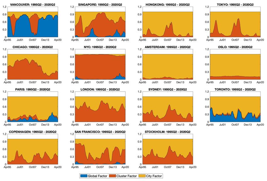
In Figure 4 we present the results of the variance decomposition analysis to investigate the relative
importance of different factors in explaining the real house price growth, and how this role has evolved over
time for each city in our sample. With the exception of Vancouver, Toronto and Paris, we find that the
common factor has not played a dominant role in explaining the real house price growth for most cities over
our sample period. This is especially true for the pre-2008 and the post-2010 sample period. This result is
consistent with our cluster analysis and suggests that a global and highly integrated housing market is not
an appropriate characterization for global cities. In contrast, we find that cluster-based factors have played
an important role in housing price growth for many cities. For example, the first cluster based latent factor
plays a significant role in the evolution of real house price growth in Singapore, Hong Kong and Tokyo. The
second cluster based factor plays a significant role for Chicago and NYC. The third cluster based factor
mainly dominates the house price growth variations in London, Sydney, San Francisco and Stockholm.
Our results also show that the role of the cluster-based factor has changed over time with a significant
increase during the financial crisis of 2008-09 for most of the cities in the sample. The result that factors
based on clusters account for a large portion of variation in real house price growth in most of the cities
during the financial crisis is also consistent with the ”tail” dependence” literature in the financial market.
For example, Zhou and Gao (2012) and Hoesli and Reka (2013) find asymmetric correlation in local and
international real estate markets during the financial crisis. Finally, for Amsterdam, Oslo, Paris, Toronto,
Hong Kong and Tokyo, the idiosyncratic factor has dominated the overall variation in real house price growth
with its share staying above 40 percent for the entire sample period. Based on this analysis we find that
the cluster-based factor plays the most important role for Singapore, Chicago, NYC, London, San Francisco
and Sydney. In terms of over time variation few other interesting patterns are worth noting. The role of
the common factor in Vancouver’s house price variations has increased over time after the financial crisis.
23 We also conducted a principal component analysis and found that the first two principal components 43 percent of the
overall variation in the housing price growth, with first component accounting for only 29 percent. These results are not included
in the paper for brevity and are available upon request.
12Although the role of idiosyncratic component has been large throughout the sample period for Toronto,
we observe a secular increase in its role, implying that Toronto’s housing market has been decoupling not
only from the global market, but also from the cluster of housing markets that it belongs to based on our
analysis. Finally, although most of the European cities are in the third cluster, this factor is most important
for housing price growth dynamics in London, Stockholm and Copenhagen.
Our findings from the variance decomposition analysis are also reinforced by the evolution of different
factors for these cities presented in Figure 5. We plot posterior means of the MCMC draws of the estimated
factors. Three key results emerge from this plot: first, all the factors witnessed a decline during the financial
crisis of 2008-09. Secondly, the length and the depth of the decline varies across different factors. The
recovery in the first two clusters was much more rapid than the third cluster. Thirdly, variations in common
factor are small compared to the other factors based on different clusters, especially, for the first and the
second cluster. In terms of the overall size of variations, the estimated factor for the third cluster that has
most of the European cities and the two cities from Canada, displays smaller variations than the other two
cluster-based factors.
Figure 6 plots estimated stochastic volatility of the estimated factors. Consistent with the findings
reported for the variance decomposition exercise, estimated stochastic volatility of the common factor shows
smaller variation than the factors based on different clusters. Not surprisingly, the volatility measure peaks
at the height of the financial crisis for all the factors. If we compare the evolution of the stochastic volatility
across different factors, we observe a significant degree of heterogeneity. The estimated stochastic volatility
shows another peak in the late 1990s for the factor based first cluster with mostly Asian cities. This is
understandable as many Asian economies were experiencing the Asian Financial crisis during this period.
The factor based on the second cluster, the variation of which is dominated by Chicago and NYC, exhibits
consistent decline in the estimated volatility after the financial crisis of 2008-09.
To summarize this section, our findings from the dynamic factor model with time-varying stochastic
volatility reinforces the results obtained in the previous section that the housing markets across the global
cities are not highly integrated with each other. Moreover, we do not find any evidence of an increased degree
of synchronization in the recent periods. Instead our findings suggest a much more segmented housing market
for global cities with clusters of cities that share housing price dynamics. This is especially true for London,
NYC, Singapore, and Sydney. Over all our findings imply substantial heterogeneity in the housing market
dynamics across global cities.
135 Discussion
A few interesting questions arise against the backdrop of our findings from Sections 3 and 4. First, why do we
find a lack of integration in housing markets of global cities? Second, what factors can explain the emergence
of clusters of cities that are more integrated with members within the cluster? Finally, what implications
can be derived for policy and investment from these two observations about the nature of housing price
dynamics for global cities?
We believe that the lack of a global market that drives house price dynamics of major international cities
is not surprising. Unlike financial markets with greater integration due to increasing financial sector openness
and regulations encouraging such synchronization, the case of housing market is different due to persistent
local affects that can influence prices as well as a regulatory environment that focuses more on local housing
needs than synchronization with other global cities.24 In recent years many major cities facing ballooning
cost of home ownership have adopted policies that either ban foreign ownership outright or discourage it via
taxation and other means. In fact, even within a country there is evidence that housing markets are not
integrated.25
One may think that geographic proximity may play a role in explaining the segmentation of global cities
housing markets into clusters with cities that have synchronized movements in housing prices. However, we
find that cities from different continents are clustered together implying factors other than geography may
be at play. For instance, there is anecdotal evidence that an influx of overseas funds may have played a big
role in the housing markets of Vancouver and Hong Kong. Hence, a common source of capital flows can
be a factor determining which markets are more synchronized. At present we are not aware of any study
that systematically investigates factors that can affect the degree of synchronization for global cities and we
believe this is an important research question for future research on this topic.26
Finally, Our findings have important implications for both policymakers as well as investors in interna-
tional real estate. In response to the housing market crash that triggered the financial recession of 2008-09,
many countries adopted macroprudential policies with the objective of reducing the systemic risk from rapid
24 Using a very long-sample, Jorda et al. (2019) have found that since 1980, house prices have tended to be much less connected
globally than equity markets.
25 For example, Miles (2019, 2020) have shown that the housing market within the U.S. and the U.K. shows a significant
degree of regionalization. Factors like population growth (Oikarinen et al., 2018), local variations in credit supply (Favara
and Imbs (2015); Cerutti et al. (2017); Mian and Sufi (2019)) and heterogeneity in housing supply elasticity (Glaeser et al.
(2008);Oikarinen et al. (2018); Paciorek (2013)) are also important determinants of house prices.
26 Note that a relative lack of easily accessible data on economic activity at city-level makes it difficult to rigorously examine
this issue. We believe a case-study approach with focused analysis of few cities in a cluster is perhaps a way forward to examine
factors that help explain why housing price cycles of certain cities in a cluster are more integrated than with those outside their
cluster.
14buildup of housing prices. Most of these policies target domestic housing conditions and in principle may
serve to reduce the degree of synchronization with foreign housing markets. Our finding that at the city-level,
the housing market is much more segmented with clusters of cities suggests that it is important to account
for such heterogeneity in the macroprudential framework. For instance, it is possible for macroprudential
policies to be more effective at taming housing price growth in housing markets with lower degree of syn-
27
chronicity with foreign housing markets (Alter et al., 2018). In terms of impact on investment behavior,
our finding of relative lack of synchronization in house prices of global cities has implications for benefits
from portfolio diversification. Real estate has emerged as an important asset class for the global investor
community. An increase in housing market integration may have benefits in terms of policy coordination,
but it creates its own set of challenges for portfolio managers in diversifying their real estate portfolios. The
results obtained in this paper suggest that portfolio diversification objectives can still be attained if we take
into account different clusters. It should also be noted that in periods of crisis like the 2008-09 financial
crisis, diversification objective is hard to achieve within the clusters given a high degree of synchronization
in housing price growth in cities in each cluster.
6 Conclusion
Contrary to the common narrative about housing markets in global cities, the analysis of house price dy-
namics presented in this paper suggests that an integrated global housing market is not an appropriate
characterization for housing markets of major international cities. Further, we do not find evidence for an
increase in the degree of synchronization in housing price dynamics over time. Our findings seem to suggest a
more segmented housing market with many city-pairs exhibiting significant phase synchronization and exis-
tence of city clusters that do not always align with geography. To understand the time-varying nature of the
role of the global and the cluster-based factors we utilize a dynamic factor model with time-varying stochastic
volatility. We find that the global factor does not play a significant role for most cities, cluster factors play
a large role for many cities, and the contribution of this factor varies over time and is state-dependent with
greater degree of synchronization within the cluster during the Great Recession of 2008-09.
27 Similar finding was supported by Funke et al. (2018) who suggest that regionally differentiated macroprudential policy such
as regional loan-to-value ratios perform best in reducing variance of housing prices in an environment with regionally segmented
housing markets.
15References
Alter, A., Dokko, J., and Seneviratne, D. (2018). House price synchronicity, banking integration, and global
financial conditions. IMF Working Paper No. 18/250.
B., D., Dewachter, H., Ferrari, S., Pirovano, M., and Van Nieuwenhuyze, C. (2016). Credit gaps in belgium:
Identification, characteristics and lessons for macro- prudential policy. Financial Stability Report 2016.
National Bank of Belgium.
Cerutti, E., Dagher, J., and Dell’Ariccia, G. (2017). Housing finance and real-estate booms: A cross-country
perspective. Journal of Housing Economics, 38:1 – 13.
Claessens, S., Ayhan Kose, M., and Terrones, M. E. (2010). The global financial crisis: How similar? how
different? how costly? Journal of Asian Economics, 21(3):247 – 264.
Claessens, S., Kose, M. A., and Terrones, M. E. (2012). How do business and financial cycles interact?
Journal of International Economics, 87(1):178 – 190.
Favara, G. and Imbs, J. (2015). Credit supply and the price of housing. American Economic Review,
105(3):958–992.
Francis, N., Owyang, M. T., and Savascin, O. (2017). An endogenously clustered factor approach to inter-
national business cycles. Journal of Applied Econometrics, 32(7):1261–1276.
Funke, M., Mihaylovski, P., and Wende, A. (2018). Out of sync subnational housing markets and macropru-
dential policies. CESifo Working Paper No. 6887.
Glaeser, E., Gyourko, J., and Saiz, A. (2008). Housing supply and housing bubbles. Journal of Urban
Economics, 64(2):198–217.
Gyourko, J., Mayer, C., and Sinai, T. (2013). Superstar cities. American Economic Journal: Economic
Policy, 5(4):167–99.
Hale, G. (2012). Bank relationships, business cycles, and financial crises. Journal of International Economics,
88(2):312 – 325.
Harding, D. and Pagan, A. (2006). Synchronization of cycles. Journal of Econometrics, 132(1):59 – 79.
Hernández-Murillo, R., Owyang, M. T., and Rubio, M. (2017). Clustered housing cycles. Regional Science
and Urban Economics, 66:185 – 197.
16Hiebert, P. and Roma, M. (2010). Relative house price dynamics across euro area and us cities: Convergence
or divergence? Working Paper No. 1206, European Central Bank.
Hirata, H., Kose, M. A., Otrok, C., and Terrones, M. E. (2012). Global house price fluctuations: Synchro-
nization and determinants. NBER Working Paper No. 18362.
Hoesli, M. (2020). An investigation of the synchronization in global house prices. Journal of European Real
Estate Research, 13(1):17–27.
Hoesli, M. and Reka, K. (2013). Volatility spillovers, comovements and contagion in securitized real estate
markets. Journal of Real Estate Finance and Economics, 47:1–35.
Hosszejni, D. and Kastner, G. (2020). Modeling univariate and multivariate stochastic volatility in r with
stochvol and factorstochvol. arXiv 1906.12123.
International Monetary Fund (2018). House Price Synchronization: What Role for Financial Factors?,
chapter 3. International Monetary Fund, Monetary and Capital Markets Department, USA.
Jorda, O., Knoll, K., Kuvshinov, D., Schularick, M., and Taylor, A. (2019). The rate of return on everything,
1870-2015. Quarterly Journal of Economics, 134(3):1225–1298.
Kallberg, J. G., Liu, C. H., and Pasquariello, P. (2014). On the price comovement of u.s. residential real
estate markets. Real Estate Economics, 42(1):71–108.
Kastner, G., Frühwirth-Schnatter, S., and Lopes, H. F. (2017). Efficient bayesian inference for multivariate
factor stochastic volatility models. Journal of Computational and Graphical Statistics, 26(4):905–917.
Katagiri, M. (2018). House price synchronization and financial openness: A dynamic factor model approach.
IMF Working Paper No. 18/209,.
Kim, S., Shephard, N., and Chib, S. (1998). Stochastic Volatility: Likelihood Inference and Comparison
with ARCH Models. The Review of Economic Studies, 65(3):361–393.
Klarl, T. (2018). Housing is local: Applying a dynamic unobserved factor model for the dutch housing
market. Economics Letters, 170:79 – 84.
Kose, M. A., Otrok, C., and Whiteman, C. H. (2003). International business cycles: World, region, and
country-specific factors. American Economic Review, 93(4):1216–1239.
17Meller, B. and Metiu, N. (2017). The synchronization of credit cycles. Journal of Banking and Finance,
82:98–111.
Mian, A. and Sufi, A. (2019). Credit supply and housing speculation. NBER Working Paper No. 24823.
Miles, W. (2017). Has there actually been a sustained increase in the synchronization of house price (and
business) cycles across countries? Journal of Housing Economics, 36:25 – 43.
Miles, W. (2019). Regional convergence and structural change in us housing markets. Regional Studies,
Regional Science, 6(1):520–538.
Miles, W. (2020). Regional uk house price co-movement. Applied Economics, 52:4976–4991.
Miles, W. H. (2015). Regional house price segmentation and convergence in the us: A new approach. Journal
of Real Estate Finance and Economics, 23:57–72.
Mink, M., Jacobs, J. P., and de Haan, J. (2012). Measuring coherence of output gaps with an application
to the euro area. Oxford Economic Papers, 64(2):217–236.
Oikarinen, E., Bourassa, S. M., and J., E. (2018). Us metropolitan house price dynamics. Journal of Urban
Economics, 105:54–69.
Otrok, C. and Terrones, M. (2005). House prices, interest rates and macroeconomic fluctuations: Interna-
tional evidence. mimeo.
Paciorek, A. (2013). Supply Constraints and Housing Market Dynamics. Journal of Urban Economics,
77:11–26.
Primiceri, G. E. (2005). Time Varying Structural Vector Autoregressions and Monetary Policy. The Review
of Economic Studies, 72(3):821–852.
Stock, J. H. and Watson, M. W. (2007). Why has u.s. inflation become harder to forecast? Journal of
Money, Credit and Banking, 39(s1):3–33.
Stock, J. H. and Watson, M. W. (2016). Dynamic factor models, factor-augmented vector autoregressions,
and structural vector autoregressions in macroeconomics. In Taylor, J. B. and Uhlig, H., editors, Handbook
of Macroeconomics, volume 2, pages 415 – 525. Elsevier.
Tsai, I.-C. (2018). House price convergence in euro zone and non-euro zone countries. Economic Systems,
42(2):269 – 281.
18Zhou, J. and Gao, Y. (2012). Tail dependence in international real estate securities markets. Journal Real
Estate Finance and Economics, 45:128–151.
19Distance
3
4
5
6
Ap
r−
0.0 0.2 0.4 0.6 0.8 1.0 1.2 19
Ap 95
r−
19
Ap 96
r−
19
Ap 97
r−
(in natural logs)
19
Vancouver Ap 98
r−
19
Ap 99
r−
Singapore Ap
20
0
r− 0
20
Ap 01
r−
Real Housing Price Index
Hong Kong 20
Ap 02
r−
20
Ap 03
Tokyo r−
20
Ap 04
r−
20
Chicago Ap 05
r−
20
Ap 06
r−
20
NYC Ap 07
r−
20
Ap 08
r−
20
Amsterdam Ap 09
r−
20
20
Ap 10
r−
Oslo 20
Ap 11
r−
20
Ap 12
r−
Paris 20
Ap 13
r−
20
Ap 14
London r−
20
Ap 15
r−
20
Sydney Ap 16
r−
20
Ap 17
Cluster 1
r−
20
1
Figure 1: Real Housing Price Index (log scale)
Ap
Toronto r− 8
20
Ap 19
r−
20
Copenhagen 20
Figure 2: City-Clusters based on similarity of housing cycles
Cluster 2
San Francisco
Stockholm
Oslo
NYC
Paris
Tokyo
Cluster 3
Sydney
Toronto
London
Chicago
Singapore
Stockholm
Vancouver
Hong Kong
Amsterdam
Copenhagen
San FranciscoCluster 1: Hong Kong, Singapore, Tokyo and Vancouver Cluster 2: Amsterdam, Chicago, NYC and Oslo
0.5
0.4
0.4
0.3
0.3
0.2
0.2
0.1
0.1
2005Q1 2007Q1 2009Q1 2011Q1 2013Q1 2015Q1 2017Q1 2019Q1 2005Q1 2007Q1 2009Q1 2011Q1 2013Q1 2015Q1 2017Q1 2019Q1
Cluster 3: Copenhagen, London, Paris, Sydney,
San Francisco, Stockholm and Toronto
0.5
0.4
0.3
2005Q1 2007Q1 2009Q1 2011Q1 2013Q1 2015Q1 2017Q1 2019Q1
Figure 3: 10-year rolling average of cluster-level phase synchronization
21Figure 4: Variance Contribution by Factor
22Figure 5: Estimated Common factor and three cluster-based factors
23Figure 6: Estimated Stochastic Volatility by Factor
24Table 1: Descriptive Statistics: 1995Q2-2020Q2
N Mean S.D. Max Min Peak Trough
Amsterdam 101 5.58 9.83 38.80 -17.56 1999 Q1 2013 Q1
Chicago 101 0.68 6.77 13.84 -21.65 2013 Q3 2009 Q1
Copenhagen 101 8.30 13.10 40.78 -28.88 2005 Q3 2009 Q1
Hong Kong 101 5.20 20.06 64.38 -54.65 1997 Q1 1998 Q1
London 101 5.95 9.51 27.28 -23.13 1999 Q4 2008 Q3
NYC 101 1.80 6.74 17.56 -14.73 2002 Q3 2008 Q3
Paris 101 6.76 10.18 30.14 -20.72 1999 Q2 2008 Q4
Oslo 101 4.46 7.88 20.69 -15.02 2010 Q4 1997 Q1
San Francisco 101 3.73 13.10 33.42 -35.25 2000 Q2 2008 Q2
Singapore 101 1.16 16.12 69.21 -40.53 2009 Q3 2009 Q1
Stockholm 101 6.12 9.09 27.38 -14.51 2000 Q2 2018 Q2
Sydney 101 4.17 10.43 32.80 -17.34 2015 Q2 2018 Q4
Tokyo 101 -1.30 6.97 18.11 -17.18 2005 Q2 2008 Q4
Toronto 101 1.74 3.88 11.60 -7.23 2016 Q3 2019 Q3
Vancouver 101 -0.81 6.80 17.79 -21.30 2017 Q3 2009 Q1
i) We report descriptive statistics for annualized growth in real housing
price index.
ii) Peak is defined as the maximum growth rate and Trough is defined as
the minimum growth rate over the sample period.
25You can also read