Accent Conversion Using Artificial Neural Networks - Stanford University
←
→
Page content transcription
If your browser does not render page correctly, please read the page content below
Accent Conversion Using Artificial Neural Networks

      Amy Bearman          Kelsey Josund        Gawan Fiore
abearman@stanford.edu kelsey2@stanford.edu gfiore@stanford.edu

                    Abstract                         features that are used for speech recognition. We
                                                     propose a system to transform speech from one ac-
    Automatic speech recognition (ASR) sys-          cent to another as a way of addressing this prob-
    tems would ideally be able to accurately         lem.
    capture speech regardless of the speaker.           In particular, we propose applying a simple
    However, accent is often a confounding           feedforward neural network with various prepro-
    factor, and having separate speech-to-text       cessing steps to learn a series of conversion weight
    models for each accent is less desirable         matrices between a source and target accent. The
    than a single model. In this paper we            resultant trained matrices accept MFCCs repre-
    propose a methodology for accent conver-         senting an utterance in one accent and output
    sion that learns differences between a pair      MFCCs for the same utterance in a different ac-
    of accents and produces a series of trans-       cent. We evaluated our model with both the mel-
    formation matrices that can be applied to        cepstral distortion measure of MFCC difference
    extracted Mel Frequency Cepstral Coeffi-         and a neural classifier to detect the degree to which
    cients. This is accomplished with a feed-        our result sequences of MFCCs truly resemble the
    forward artificial neural network, accom-        desired accent.
    panied by alignment preprocessing, and
                                                        Theoretically, an ASR system could be imple-
    validated with MCD and a softmax classi-
                                                     mented with a separate model for each anticipated
    fier. Results show that this approach may
                                                     accent. Compared to our approach, this would re-
    be a useful preprocessing step for ASR
                                                     quire the same number of trained models (one for
    systems.
                                                     each accent). However, our approach requires sig-
1   Introduction                                     nificantly less training data, and thus less training
                                                     time, because it breaks out the accent portion of
Among the many issues facing Automatic Speech        the overall speech recognition problem, avoiding
Recognition (ASR) systems, effectively handling      duplication of the rest of the training necessary for
accents is one of the most challenging. Partic-      speech recognition.
ularly when working with languages that have            This issue of understanding varied accents
highly varied pronunciations, such as Spanish, En-   arises in most languages, and, accordingly, the ap-
glish, and Chinese [17], an ASR system trained on    proach we use could be applied to any language.
only one accent might only be effective for a mi-    However, for simplicity of development and due
nority of the speakers of that language. This does   to available training data, we trained and tested our
not include non-native speakers who learn a lan-     model on the English language with American, In-
guage and carry over their native accent, a popu-    dian, and Scottish accents, for both genders.
lation that expands the need for proper handling
of accent variation. Frequently, ASR systems per-    2   Background and Related Work
form much better for users with the same accent as
the training data used to develop the system. This   Voice conversion is an active area of research, but
is due to the way accents affect prosody, enunci-    the majority of papers on the subject focus on
ation, vowel sounds, and other aspects of speech,    modifying the voice itself, not the pronunciation.
which in turn change the resulting MFCC or other     [9], [10], and [11] demonstrate that it is possi-
ble to reconstruct a speech sound from mel fre- dio variations over different time spans, with the
quency cepstral coefficients, although it typically goal of capturing both short term features and long
requires additional inputs for accurate reconstruc- term dependencies. A 3-tiered flavor of this ap-
tion. [10] used a pitch excitation signal in con- proach was greatly preferred by AB test subjects
cert with MFCCs as an input into a source-filter over both an unconditional RNN solution and a
model which resulted in more natural-sounding WaveNet implementation.
speech. [11] similarly used pitch data, but they We take particular inspiration from [16], which
instead derived sine-wave frequencies from the compared a GMM model to an ANN model to
pitch and used this to invert the original binning convert a female voice to a male one with the same
step in MFCC computation. [15] compared per- utterance. This study used the same dataset we
formance of Gaussian Mixture Models to DNNs have access to, making their results particularly
map of spectral features of a source speaker to that relevant to us. They also showed that a remarkably
of a target speaker, converting the speaking voice simple model can perform very well in this prob-
while maintaining the content of speech. They lem space. One further major area of related work
used f0 transformation for both models and opti- is in accent classification. This is the problem
mized mean squared error of transformed MFCCs of inferring the native language or regional iden-
in the neural network and found that the best re- tity of a speaker from his or her accented speech.
sults were obtained with a four-hidden-layer neu- Similar features that allow for accent identifica-
ral network with hidden layers of variable size. tion/classification are relevant for accent conver-
[14] applied Convolutional Neural Networks to sion since the aspects of an accent that character-
the same problem in an attempt to modify not ize it are precisely what must be changed for con-
just pitch but also timbre, with the intent of im- version. Further, to identify whether an accent has
proving the similarity between the target speaker’s been successfully reconstructed after a conversion
voice and the generated voice. They both trans- process, a classifier is very useful.
formed speech directly and built generative mod- Spectral features and temporal features such as
els to sound like a particular person through use of intonation and durations vary with accent. These
generative adversarial networks and visual anal- features have been used in statistical models such
ogy construction. [13] employed deep autoen- as Gaussian Mixture Models (GMMs) and Hid-
coders to train in a speaker-independent fashion, den Markov Models (HMMs) to discriminate be-
which allowed them to build representations of tween several different accents. [3] used GMMs
speaker-specific short-term spectra. They ulti- trained with formant frequency features to dis-
mately modified input voices to match some target criminate between American English and Indian
voice and performed both objective (reconstruc- accented English. [2] identified Flemish regional
tion error) and subjective (human perception) eval- accents by providing formant and phoneme dura-
uations. All three of these neural-net-based voice tion features as input to the eigenvoice method [5],
modification projects have a similar intuition to which is a dimensionality reduction technique for
what we propose, but they do not deal with accents speaker models. [6] proposes a linear discriminant
broadly but rather more specifically individuals. analysis (LDA) approach (essentially, a form of
dimensionality reduction) on individual phoneme
Neural networks (particularly deep neural net- classes and extended to continuous speech utter-
works) have been shown to be particularly effec- ances, in order to classify three different types of
tive for representing sequential information such accents. [7] and [8] used support vector machines
as language, video, and speech. Generally, DNNs (SVMs); [7] trained SVMs with MFCC features
also serve as accurate classifiers. [12] used both and [8] trained using word-final stop closure du-
DNNs and RNNs together in a single classifier ration, word duration, intonation features, and the
to identify accents, with the DNN focused on F2-F3 contour which captures tongue movements.
longer term statistical features and the RNN on
shorter term acoustic features. They found that 3 Approach
this system outperformed either DNNs or RNNs
when used alone. [16] created an audio gener- We used parallel utterances from American, In-
ation model using hierarchical RNNs that con- dian, and Scottish English, extracted MFCCs,
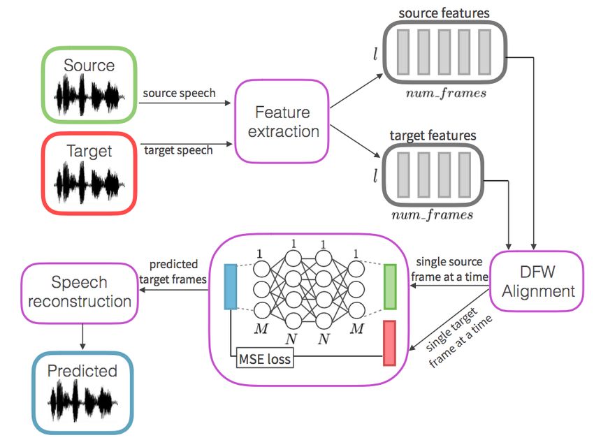
sisted of different modules focused on learning au- aligned them using fast dynamic time warping(FastDTW), and fed the resultant features through
a feedforward neural network to learn conversion
weight matrices.
3.1 Dataset
The CMU Arctic dataset consists of 1150 sam-
ples of text spoken by men with American, Cana-
dian, Scottish, and Indian accents, and a woman
with an American accent. Since the American and
Canadian accents sounded nearly identical to our
ears, we used only the American accent for this Figure 1: Architecture diagram of feedforward
project. We extracted 25 mel cepstral coefficients neural network
from each 5ms frame with 100 frequency bands in
each of the training samples and paired samples Specifically, our model involved the following
of identical utterances in two different accents for computations on the prediction step:
the source and target data into our system. Each
feature vector was zero-padded or truncated to the z = input M F CCs · W1
same length, which we set to be 1220 frames per
sample. h1 = tanh(z)
z = h1 · W 2
3.2 Alignment
h2 = tanh(z)
After extracting the MFCCs, the source and target
predicted M F CCs = h2 · W3
were aligned using FastDTW. This is an O(N) time
approximate alignment algorithm that minimizes
Note the lack of a nonlinearity on the final
squared error between the two samples. Align-
prediction layer. All weights are learned for all
ment is necessary because people speak at differ-
timesteps in the data simultaneously, allowing the
ent rates and without alignment it is much harder
lack of temporal awareness by the feedforward ar-
for the system to identify which differences are
chitecture to not be a handicap in learning.
due to accent and which are due to rate of speech.
3.4 Waveform Reconstruction
After predicting MFCCs for the target accent, we
3.3 Artificial Neural Network reconstructed the waveform using a MatLab im-
plementation of InvMFCC. This is a lossy func-
We constructed a feedforward neural network tion, as MFCCs do not retain all information about
with two hidden tanh layers of size 100 and a speech sounds that are perceivable, so the resultant
final linear output layer. Both the input layer and waveforms were guttural and noisy. Pitch infor-
output layer were of size 25, since we used 25 mation in particular is lost in the MFCC transfor-
coefficients from each 5-millisecond time period. mation.
The model learned the weight matrices for the
two hidden layers and the output layers, which 4 Experiments
started with xavier initialization, and we found 4.1 ANN Model
that performance was much better when trained
without biases. Figure 1 explains this in more 4.1.1 Architecture
detail, including pre-and post-processing steps. Our final model used Adam optimization to mini-
mize mean squared error over 5,000 epochs withbatch size 16. We first tried basic gradient de- actual samples from that accent. This possibly in-
scent, then noted that papers frequently made use dicates that the learned matrices successfully con-
of momentum for similar tasks and used Tensor- vert accents into an archetype of the target which
Flow’s MomentumOptimizer before trying Adam is apparently more strongly associated with the ac-
optimization. After experimentation with various cent’s features than the speech of an individual
learning rates, batch sizes, numbers of epochs, and who speaks with that accent. Alternatively, it is
momentum values, we found that similar hyperpa- possible that both the classifier and the converter
rameters worked for all three of our dataset pairs learn the same patterns between accents, result-
(US-Scottish, US-Indian, US female-US male). ing in artificially high performance. The very high
We evaluated our model, as in [16], with Mel accuracy also stems from the rather small sample
Cepstral Distortion, which is a weighted average size of converted files.
of squared differences between two sets of mel
frequency cepstral coefficients attuned to the
perception of the human ear. 4.1.3 Results
q
10 P24 (i) (i)
M CD = ln10 2 i=0 (mc1 − mc2 )2 Our model achieved MCDs below 10 for all three
of the conversions we attempted. The state of the
art for voice gender conversion is 6.9, which we
4.1.2 Classifier were able to approach; there is no benchmark for
To evaluate our model’s performance, we created accent conversion, but our MCD scores are quite
a softmax classifier to predict an accent label from close for that task as well.
MFCC data parsed identically to the parsing in
our primary conversion model. This took the form
of a feedforward ANN with two hidden tanh lay- Accents Train MCD Val MCD
ers and a softmax output, with hidden sizes 750 US to Scottish 9.67 9.84
and 1000 and cross entropy loss. The classifier US to Indian 8.93 8.93
achieved 92.9% accuracy in binary classification US female to male 8.16 8.17
on the benchmark American English versus Scot-
tish English task, significantly outperforming the Table 3: MCD Results
68% accuracy of a Naive Bayes classifier and 76%
accuracy of a Support Vector Machine classifier
for the same problem. Figure 2 shows the similarity between the
frequencies of predicted and target utterances
Accents Accuracy CE Loss and Figure 3 demonstrates the same comparison
US to Scottish 92.9 % 0.06 for the waveforms. Frequencies and waveforms
US to Indian 95.1 % 0.07 for these plots were both computed after MFCC
US female to male 90.7 % 0.11 computation and conversion back to a wave
file for both target and prediction to eliminate
Table 1: Baseline results of classifier on CMU disparities due to the lossy nature of MFCC calcu-
Arctic data lation. The differences between the prediction and
target are visible, but the general shape for both
Accents Accuracy CE Loss the frequencies and the wave form are similar
US to Scottish 95.9 % 0.06 between the two.
US to Indian 98.2 % 0.07
US female to male 100 % 0.1
Table 2: Results of classifier on 200 converted
samples
The performance of our classifier on the trans-
formed wave files shows that they in general are Figure 2: frequencies for prediction and target
more representative of their target accent than areing them for all sound files in our original CMU
Arctic dataset, then trained by pairing the MFCC-
only file as input with its original as the target. The
goal was to have the model learn restorative trans-
formation matrices that would negate the observed
degradation patterns of MFCC-InvMFCC conver-
Figure 3: waveforms for prediction and target sions and then apply those transformation matrices
to the waveform output of our accent conversion
4.2 Other Methods Tried model. While this showed modest success in sub-
4.2.1 Sequence-to-Sequence LSTM-RNN jective sound quality, it was not quantifiable.
The first method we used to approach this problem
was a sequence-to-sequence LSTM-RNN, build- 4.2.4 Alternative Features
ing off of the intuition of neural machine trans- Given the poor reconstruction abilities of MFCCs,
lation. We hoped to learn a statistical represen- we also experimented with training on raw wave
tation of each accent which could then be used files and on Fourier Transform features. Using just
to generate the same utterance in a new accent. 1/16000-second-long samples from the raw wave
This would have the benefit of taking advantage form was the simplest method tried since it re-
of temporal information in the utterances that is quired no processing or reconstruction at the end,
lost in a feedforward architecture. Initial results but it performed poorly since alignment has little
were no more promising than the simpler feedfor- meaning on a vector of this form and there is too
ward model, however, and we had more literature much variation to learn. The Fast Fourier Trans-
to back up focusing on that model for this particu- form algorithm is quick and fully invertible via
lar problem. the Inverse Fast Fourier Transform, which is an
attractive quality since we need to revert back to a
4.2.2 Denoising Autoencoder wave form from a feature vector. Models trained
Denoising autoencoders (DAEs) are unsupervised on Fourier Transform data performed better than
models that learn how to reconstruct their input MFCC-based models after a few epochs, but then
and remove some added noise at the same time. ceased to continue to learn.
They consist of an encoding step and a decod-
ing step which operate on the same learned weight 5 Conclusion and Future Work
matrices and bias vectors. We hoped to learn two
DAEs, one for the source and one for the target The feedforward architecture successfully con-
accents, and then use the learned weight matrices verts the MFCCs of a sample from one accent
for each of these to encode one accent and decode to another, but loses other speech characteris-
it into the other. Our DAE successfully denoised tics that are not represented by MFCCs. Future
each of the input accents back into itself, but was work should focus on integrating other features
less useful for accent modification. This could be into the model to use in reconstruction, perhaps
a good avenue for future research. starting with rescaling the wavefiles reconstructed
from the predicted MFCCs using pitch data of
4.2.3 Post-MFCC-Reconstruction some kind. Alternatively, the waveform degrada-
Improvement tion problem might be solved if similarly success-
All of our three attempted model architectures ful accent conversion could be achieved with less
learned best with MFCC features, but the MFCC lossy features than MFCCs.
and inverse MFCC process is very lossy so re- While the results of the simple feedforward
constructed sound files do not sound natural. We model are gratifying, more complex models
therefore built a postprocessing model with simi- should be able to capture additional information
lar intuition and architecture to our most success- about utterances and accents that this model does
ful feedforward ANN that, rather than learning to not. The intuition behind denoising autoencoders
convert one accent to another, learned to convert a seems extremely relevant to this problem space,
wavefile that resulted from the MFCC-InvMFCC suggesting that there is some implementation that
process to the original wavefile. We created train- would lead to greater success. Particularly, learn-
ing data by computing the MFCCs and then invert- ing with additional or alternative features besidesMFCCs may be more successful with such archi- accent discrimination models and comparisons
tectures. The ability of RNNs to capture tempo- with human perception benchmarks, in Proc.
ral information should also be further explored, as EuroSpeech, vol. 4, pp. 23232326, 1997.
such information is certainly relevant to the differ-
ences between accents. [7] H. Tang and A. A. Ghorbani, Accent
As discussed in the introduction, however, classification using support vector machine and
one of the primary uses of a system such as hidden markov model, in Advances in Artificial
this would be as an initial processing step in a Intelligence. Springer, 2003, pp. 629631.
speech recognition system. In that case, the poor
reconstruction of the wave file may not matter; [8] C. Pedersen and J. Diederich, Accent
all that would be required would be accurately classification using support vector machines, 6th
predicting the features used by the rest of the Intl. Conf. on Comp. and Info. Sc., 2007.
system. In that case, additional hyperparameter
tuning or additional data acquisition would be [9] G. Min, X. Zhang, J. Yang, and X Zou,
useful to drive the MCD score lower, indicating Speech reconstruction from mel-frequency cep-
even more faithful accent conversion. stral coefficients via 1-norm minimization, in
IEEE 17th International Workshop on Multimedia
Signal Processing (MMSP), 2015.
6 References
[1] L. M. Arslan and J. H. Hansen, Frequency [10] B. Milner, X. Shao, Speech reconstruc-
characteristics of foreign accented speech, in tion from mel-frequency cepstral coefficients
Proc. ICASSP. IEEE, 1997, pp. 1123 - 1126. using a source-filter model, School of Information
Systems, University of East Anglia, Norwich, UK.
[2] P.-J. Ghesquiere and D. Van Compernolle,
Flemish accent identification based on formant [11] Dan Chazan, Ron Hoory, Gilad Cohen
and duration features, in Acoustics, Speech, and and Meir Zibulski, Speech reconstruction from
Signal Processing (ICASSP), IEEE International mel-frequency cepstral coefficients and pitch
Conference on, vol. 1. Orlando, FL, USA: IEEE, frequency, IBM Research Laboratory in Haifa.
2002, pp. 749.
[12] Yishan Jiao, Ming Tu, and Julie Liss,
[3] S. Deshpande, S. Chikkerur, and V. Accent Identification by Combining Deep Neural
Govindaraju, Accent classification in speech, in Networks and Recurrent Neural Networks Trained
Automatic Identification Advanced Technologies, on LSTM, Arizona State University.
Fourth IEEE Workshop on. Buffalo, NY, USA:
IEEE, 2005, pp. 139143. [13] Seyed Hamidreza Mohammadi and
Alexander Kain, Voice Conversion Using Deep
[4] Y. Zheng, R. Sproat, L. Gu, I. Shafran, Neural Networks with Speaker-Independent
H. Zhou, Y. Su, D. Jurafsky, R. Starr, and S.-Y. Pre-Training, Center for Spoken Language Un-
Yoon, Accent detection and speech recognition derstanding, Oregon Health & Science University,
for shanghai-accented mandarin. in Interspeech. IEEE.
Lisbon, Portugal: Citeseer, 2005, pp. 217220.
[14] Shariq A. Mobin and Joan Bruna, Voice
[5] R. Kuhn, P. Nguyen, J.-C. Junqua, R. Bo- Conversion using Convolutional Neural Net-
man, N. Niedzielski, S. Fincke, K. Field, and M. works, UC Berkeley.
Contolini, Fast speaker adaptation using a priori
knowledge, in Proc. International Conference on [15] Srinivas Desai, E. Veera Raghavendra,
Acoustics, Speech and Signal Processing, March B. Yegnanarayana, Alan W Black, Kishore Pra-
1999, vol. II, pp. 749752. hallad, Voice Conversion Using Artificial Neural
Networks, International Institute of Information
[6] K. Kumpf and R. W. King, Foreign speaker Technology - Hyderabad, India.
accent classification using phoneme-dependent[16] Soroush Mehri, Kundan Kumar, Ishaan Gulrajani, Rithesh Kumar, Shubham Jain, Jose Sotelo, Aaron Courville, Yoshua Bengio, Sam- pleRNN: An Unconditional End-to-End Neural Audio Generation Model, ICLR 2017. [17] Yanli Zheng, Richard Sproat. ”Accent Detection and Speech Recognition for Shanghai- Accented Mandarin.” DBLP January 2005.
You can also read