Day 3: Diagnostics and Output - Adam Phillips - CESM
←
→
Page content transcription
If your browser does not render page correctly, please read the page content below
Day 3: Diagnostics and Output

                 Adam Phillips
                 asphilli@ucar.edu
Climate Variability and Change Working Group Liaison

         Thanks to Alice Bertini and Dave Bailey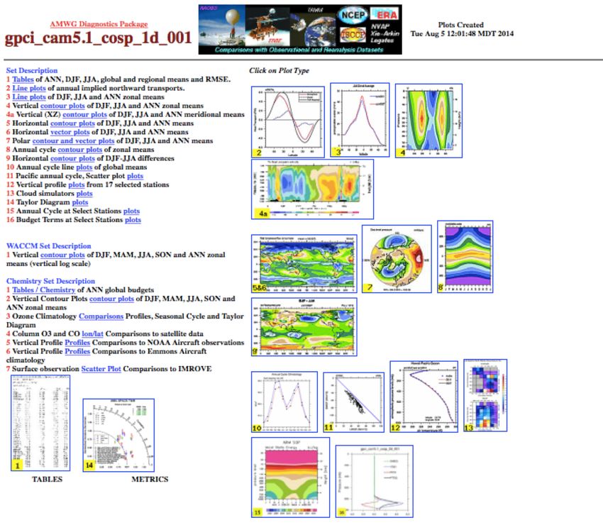
Outline
I.  CESM2 output data and experiments
II. Introduction to the netCDF format, ncdump
III.netCDF Operators (NCO) and Climate Data Operators (CDO)
IV. Quick-use tools: ncview, panoply, ImageMagick, ghostview,
    xxdiff
V. Introduction to NCL
VI. Practical Lab #3
    A. Diagnostics packages
    B. NCL post-processing scripts
    C. NCL graphics scripts
    D. Additional Exercises
    E. Challenges

                     Day 3 - 2018 CESM Tutorial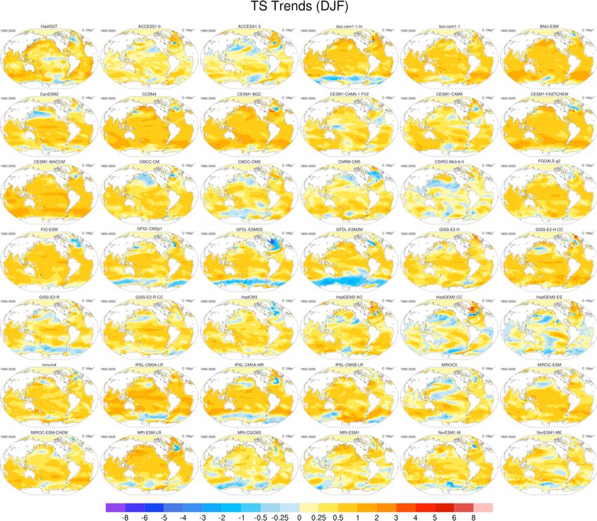
Short-term Archive and Run Directories

                             /glade/scratch/

 Short-term                                         /$CASE
                     /archive/$CASE                                Run Directory
 Archive Directory

  atm       lnd      ocn    ice     cpl                      bld    run

   logs     glc      rest   esp     rof    wave

I. CESM2 output data and experiments
                             Day 3 - 2018 CESM Tutorial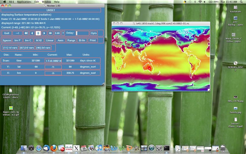
Short-term Archive Directory

                             /glade/scratch/

                    /archive/$CASE

                                          - By default, short term archiver writes to
                                          /glade/scratch//archive/$CASE
                                          on cheyenne. To modify this path set
                                          DOUT_S_ROOT in env_run.xml.

                                              - As of CESM2 long term archiving can
  atm      lnd      ocn     ice     cpl
                                              no longer be used.

   logs    glc     rest    esp      rof    wave

I. CESM2 output data and experiments
                             Day 3 - 2018 CESM Tutorial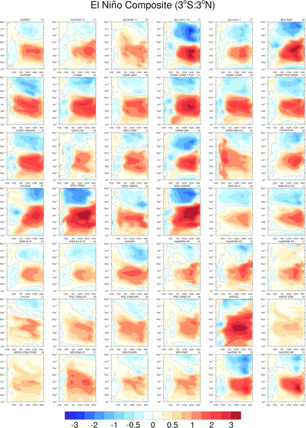
CESM History File Naming Conventions
   All history output files are written in NetCDF format.
   Location of history files in short-term archive directory:
   /glade/scratch//archive/$case//hist
           component = atm, ocn, etc.
   CESM distinguishes between different time sampling frequencies by creating
   distinct history files for each frequency. Sampling frequencies are set by the
   user within the namelist.
   Example history file names:
      f40_test.cam.h0.1993-11.nc f40_test.clm2.h0.1993-11.nc
      f40_test.pop.h.1993-11.nc  f40_test.cice.h.1993-11.nc
   By default, h0/h denotes that the time sampling frequency is monthly.
   Other frequencies are saved under the h1, h2, etc file names:
   f40_test.cam2.h1.1993-11-02-00000.nc

I. CESM2 output data and experiments
                             Day 3 - 2018 CESM Tutorial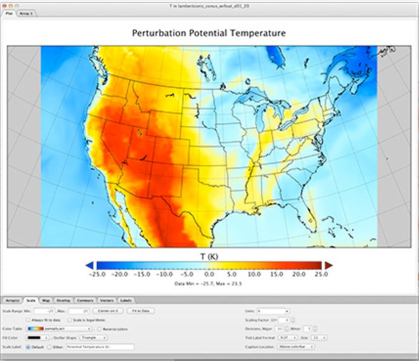
CESM History Files vs. Timeseries Files
   History files contain all variables for a component for a particular frequency,
   and are output directly from the model.
   Timeseries files are created offline from the model, either by the official CESM
   workflow post-processing scripts (limited support, run on Cheyenne/DOE
   machines), or by individual user-generated scripts. Timeseries files span a
   number of timesteps, and contain only one (major) variable.
   Timeseries files are considerably more useful in day-to-day research and are
   regularly distributed while history files are not.
   Example history file: f40_test.cam.h0.1993-11.nc
               - 1 monthly timestep (Nov. 1993)
               - 200+ CAM variables (ex. PSL, TS, PRECC..)

   Example timerseries file: f40_test.cam.h0.PSL.199001-199912.nc
              - 120 monthly timesteps (Jan 1990 – Dec 1999)
              - 1 CAM variable (PSL), along with auxiliary variables (time,lat,etc.)

I. CESM2 output data and experiments
                             Day 3 - 2018 CESM Tutorial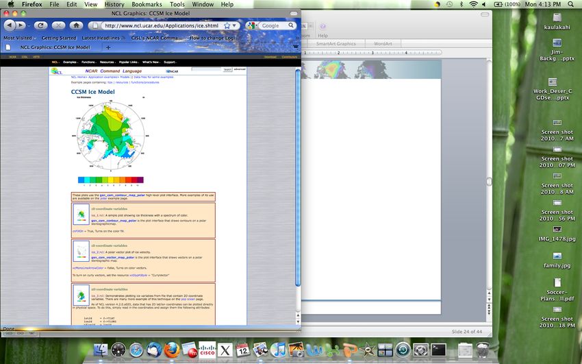
CESM CMIP5/6 Files
   CESM CMIP files are similar to CESM timeseries files.
   Example CMIP file: clt_Amon_CESM1-CAM5_historical_r1i1p1_185001-200512.nc
              - 1872 monthly timesteps (Jan 1850 – Dec 2005)
              - 1 variable (clt), along with auxiliary variables (time,lat,etc.)
   CESM CMIP files are designed to match CMIP/CMOR conventions, and thus
   metadata and auxiliary variables (ex. time) may not match CESM timeseries
   files.
   CMIP variables may be a 1-to-1 match to CESM variables, or they may not be.
   Examine the data/metadata to check.

I. CESM2 output data and experiments
                             Day 3 - 2018 CESM Tutorial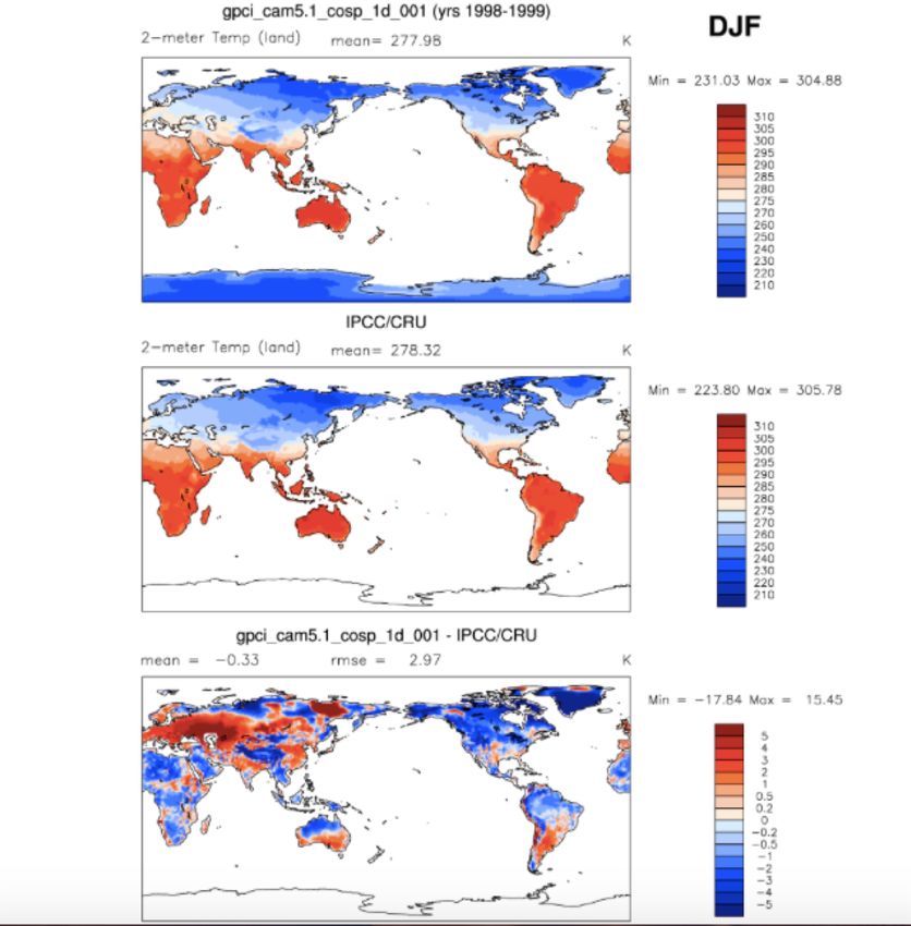
CESM & time variable
   The time coordinate variable in CESM history files represents the end of the
   averaging period for variables that are averages.
   This is different from the time expressed in the file name. For monthly files, the
   time given in the file name is correct.

   Example File: f.e11.FAMIPC5CN.f09_f09.rcp85.ersstv5.toga.ens10.cam.h0.2017-12.nc
   When the time
   coordinate variable is
   translated, the time is
   00Z January 1st 2018,
   even though the file
   holds averaged
   variables for
   December 2017.

I. CESM2 output data and experiments
                             Day 3 - 2018 CESM Tutorial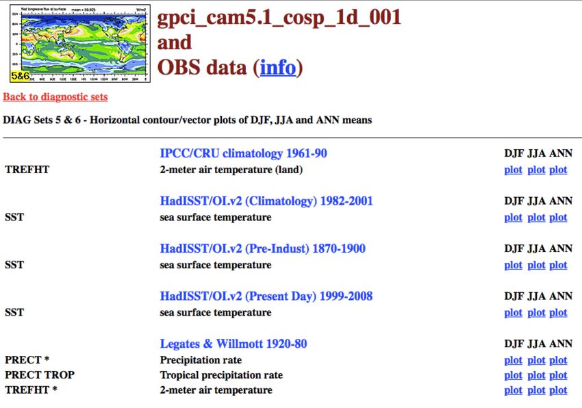
CESM & time variable
   To verify the averaging period in the files, consult the time_bnds, time_bound
   or time_bounds variables in the file.

   Example File: f.e11.FAMIPC5CN.f09_f09.rcp85.ersstv5.toga.ens10.cam.h0.2017-12.nc
   When the time_bnds
   variable is translated,
   the time averaging
   period is shown to be
   from 00Z Dec 1st
   2017 through 00Z
   Jan 1st 2018.

   Why is this done? The time is set at the end of the averaging period, and as
   CESM allows instantaneous variables to be saved with average variables the
   time is also the correct time for instantaneous variables.
   Discussions are ongoing as to how this might change for CESM2 output.
   Regardless of what happens, always verify the averaging period as shown above.

I. CESM2 output data and experiments
                             Day 3 - 2018 CESM Tutorial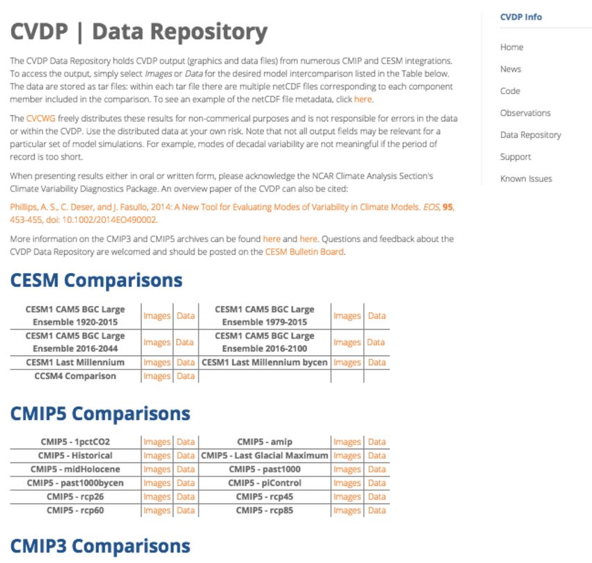
CESM Experiments Websites

                        http://www.cesm.ucar.edu/experiments/
I. CESM2 output data and experiments
                             Day 3 - 2018 CESM Tutorial
CESM Experiments Websites
http://www.cesm.ucar.edu/experiments/
I. CESM2 output data and experiments
Day 3 - 2018 CESM TutorialCESM Experiments Websites
Links to the Climate
Data Gateway (formerly
the Earth System Grid)
http://www.cesm.ucar.edu/experiments/
I. CESM2 output data and experiments
Day 3 - 2018 CESM TutorialClimate Data Gateway at NCAR
Publicly released
CESM data is available
via the CDG.
Registration is quick
and easy. NCAR
accounts are not
required.
Timeseries data in
CESM and CMIP
formats are available.
I. CESM2 output data and experiments
Day 3 - 2018 CESM TutorialConcise and reliable expert guidance on the strengths,
limitations and applications of climate data…
http://climatedataguide.ucar.edu
Describe observations used for Earth System
Model evaluation; 150+ data sets profiled
Data set pros and cons evaluated by
nearly 4 Dozen Experts
(‘expert-user guidance’)
Comparisons of many common variables:
SST, precipitation, sea ice concentration,
atmospheric reanalysis, etc.
Comparison of SST data sets and their recent
trends in the tropical Pacific 140,000 unique visitors in 2014
(up from 41,000 in 2012)
For more info contact David P. Schneider, NCAR, Climate Analysis Section. dschneid@ucar.edu
Day 3 - 2018 CESM TutorialIntroduction to NetCDF
netCDF stands for “network Common Data Form”
PROS: self-describing, portable, metadata friendly, supported by many
languages including fortran, C, Matlab, ferret, GrADS, NCL, IDL, python; viewing
tools like ncview/panoply; and tool suites of file operators (NCO, CDO).
CONS: compression not available until netCDF4, oftentimes requires users to
explicitly access information (not true in NCL)
http://www.unidata.ucar.edu/software/netcdf
http://www.unidata.ucar.edu/software/netcdf/docs/BestPractices.html
II. Introduction to the netCDF format, ncdump
Day 3 - 2018 CESM Tutorialnetcdf slp.mon.mean {
dimensions:
ncdump lon = 144 ;
lat = 73 ;
time = UNLIMITED ; // (744 currently)
variables:
ncdump is a netCDF utility that float lat(lat) ;
lat:units = "degrees_north" ;
allows one to dump the contents lat:actual_range = 90.f, -90.f ;
of the netCDF file to screen or lat:long_name = "Latitude" ;
file. float lon(lon) ;
lon:units = "degrees_east" ;
To view the header of a netCDF file: lon:long_name = "Longitude" ;
ncdump –h slp.mon.mean.nc lon:actual_range = 0.f, 357.5f ;
double time(time) ;
time:units = "hours since 1-1-1 00:00:0.0" ;
To view the contents of a variable: time:long_name = "Time" ;
time:actual_range = 17067072., 17609832. ;
ncdump –v slp slp.mon.mean.nc | float slp(time, lat, lon) ;
less slp:long_name = "Sea Level Pressure" ;
slp:valid_range = 870.f, 1150.f ;
slp:actual_range = 960.1486f, 1082.558f ;
To view the netCDF file type: slp:units = "millibars" ;
ncdump –k slp.mon.mean.nc slp:missing_value = -9.96921e+36f ;,
// global attributes:
result: netCDF-4 :title = “Monthly mean slp from the NCEP Reanalysis" ;
:description = "Data is from NMC initialized reanalysis\n
"(4x/day). These are the 0.9950 sigma level values." ;
:Conventions = "COARDS" ; }
II. Introduction to the netCDF format, ncdump
Day 3 - 2018 CESM TutorialnetCDF Operators (NCO)
NCO is a suite of programs designed to perform certain “operations” on
netCDF files, i.e., things like averaging, concatenating, subsetting, or
metadata manipulation.
Command-line operations are extremely useful for processing model data
given that modelers often work in a UNIX-type environment.
UNIX wildcards are accepted for many of the operators.
The NCO’s recognize missing data by the _FillValue attribute.
(missing_value is ignored.)
The NCO Homepage and Reference Manual can be found at
http://nco.sourceforge.net
Note: There are many other netCDF operators beyond what will be
described here.
III. NCO netCDF Operators / CDO Climate Data Operators
Day 3 - 2018 CESM TutorialnetCDF Operators (NCO)
NCRA (netCDF record averager)
Example: ncra file1.nc file2.nc avgfile.nc
file1.nc = input model history file, for jan year 1
file2.nc = input model history file, for feb year 1
avgfile.nc = new file consisting of jan/feb averaged data for all
fields found in the input model history file.
NCRCAT (netCDF record concatenator)
Examples: ncrcat file1.nc file2.nc out12.nc
out12.nc = new model history time series file consisting of the months of
jan and feb, year 1. Each time-varying field in this file now has
2 time steps.
III. NCO netCDF Operators / CDO Climate Data Operators
Day 3 - 2018 CESM TutorialIntroduction to netCDF Operators (NCO)
NCEA (netCDF ensemble averager)
Example: ncea amip_r01.nc amip_r02.nc amip_r03.nc amip_ENS.nc
amip_r01.nc = input file from ensemble member #1
containing monthly Jan-Dec year 1 data
amip_r02.nc = same as above but contains data from ensemble member #2
amip_r03.nc = same as above but contains data from ensemble member #3
amip_ENS.nc = new file consisting of monthly Jan-Dec year 1 data
averaged across the 3 ensemble members.
NCDIFF (netCDF differencer)
Example: ncdiff amip_r01.nc amip_r02.nc diff.nc
diff.nc = contains the differences between amip_r01.nc and amip_r02.nc.
Note: Useful for debugging purposes.
III. NCO netCDF Operators / CDO Climate Data Operators
Day 3 - 2018 CESM TutorialIntroduction to netCDF Operators (NCO)
NCKS (netCDF “Kitchen Sink” = does just about anything)
Combines various netCDF utilities that allow one to cut and paste subsets of data
into a new file.
Example: ncks –v TEMP f40_test.pop.h.1993-11.nc f40_test.TEMP.199311.nc
f40_test.pop.h.1993-11.nc = input model history file (monthly)
-v TEMP = only grab the TEMP variable
f40_test.TEMP.1993-11.nc = output file containing TEMP + associated
coordinate variables
Note #1: Only those variables specified by –v and their associated coordinate variables
are included in the output file. As the variables date, TLAT, and TLONG are not
coordinate variables of TEMP, they won’t be copied to the output file unless one does
this:
ncks –v TEMP,date,TLAT,TLONG f40_test.pop.h.1993-11.nc f40_test.T.1993-11.nc
Note #2: Wildcards not accepted.
III. NCO netCDF Operators / CDO Climate Data Operators
Day 3 - 2018 CESM TutorialIntroduction to netCDF Operators (NCO)
Other commonly used operators:
NCATTED (attribute editor)
NCRENAME (rename variables, dimensions, attributes)
NCFLINT (interpolates data between files)
NCPDQ (pack to type short or unpack files)
III. NCO netCDF Operators / CDO Climate Data Operators
Day 3 - 2018 CESM TutorialIntroduction to netCDF Operators (NCO)
netCDF operator options
-v Operates only on those variables listed.
ncks –v T,U,PS in.nc out.nc
-x –v Operates on all variables except those listed.
ncrcat –x –v CHI,CLDTOT 1999-01.nc 1999-02.nc out.nc
-d Operates on a subset of data.
ncks -d lon,0.,180. -d lat,0,63 in.nc out.nc
Real numbers indicate actual coordinate values, while integers
indicate actual array indexes. In the above example, all longitudes will
be grabbed from 0:180E, and the first 64 latitudes indexes will be
grabbed.
-h Override automatic appending of the global history attribute with the NCO
command issued (which can be very long)
More options exist beyond what was discussed here.
III. NCO netCDF Operators / CDO Climate Data Operators
Day 3 - 2018 CESM TutorialIntroduction to netCDF Operators (NCO)
Note that you can wrap the NCO’s into a script
begin
syear= "1920" ; YYYY
eyear ="2029" ; YYYY
emonth = "12"
time_s = "{1,2}*" ; "0*" = default, {1,2}* for 20C simulations
mrun = "b.e11.B20TRLENS_RCP85.f09_g16.xbmb.011"
indir = "/glade/scratch/dbailey/archive/"+mrun+"/"
outdir = "/glade/scratch/asphilli/"+mrun+"/"
atm_vars = (/“PSL”,”PRECC","PRECL","TS"/)
;——————————————————————————————————————
if (.not.fileexists(outdir)) then
system("mkdir "+outdir)
end if
do gg = 0,dimsizes(atm_vars)-1
ofile = outdir+mrun+".cam.h0."+atm_vars(gg)+"."+syear+"01-"+eyear+emonth+".nc”
system("ncrcat –h -v "+atm_vars(gg)+" "+indir+"atm/hist/*.h0."+time_s+" "+ofile+” &")
end do
end
III. NCO netCDF Operators / CDO Climate Data Operators
Day 3 - 2018 CESM TutorialIntroduction to Climate Data Operators (CDO)
CDO are very similar to the NCO. Within the CDO library there are over 600
command line operators that do a variety of tasks including: detrending,
EOF analysis, meta data modification, statistical analysis and similar
calculations.
CDO are not currently used in the diagnostics packages, so we will not go
into specifics here. We mention the CDO to make you aware of their
existence.
The CDO Homepage can be found at:
https://code.zmaw.de/projects/cdo/
CDO documentation can be found at:
https://code.zmaw.de/projects/cdo/wiki/Cdo#Documentation
III. NCO netCDF Operators / CDO Climate Data Operators
Day 3 - 2018 CESM Tutorialncview
ncview is a graphical interface
which allows one to quickly view
the variables inside a netCDF file.
Example: ncview file1.nc
ncview allows you to interactively
visualize a selected variable across
a selected range (time, spatial).
IV. Quick-use tools
Day 3 - 2018 CESM TutorialPanoply
Panoply is another GUI
application that allows one to
quickly view data in a netCDF,
HDF, or GRIB format (amongst
others). Similar to ncview, but
more powerful, panoply allows
the user to perform simple
calculations, apply masks, and to
quickly create spatial or line
plots.
Note: v4.9.3 requires Java SE 8
runtime environment or newer.
Limited documentation, but
numerous demonstration
tutorials/videos.
The Panoply homepage can be found at:
http://www.giss.nasa.gov/tools/panoply/
IV. Quick-use tools
Day 3 - 2018 CESM TutorialImageMagick
ImageMagick is a free suite of software that that can be used to display,
manipulate, compare or convert images. It can also be used to create movies.
There are two ways to use ImageMagick. One way is to simply display the
image and alter it using pop-up menus visible after clicking on the image:
display plot1.png
A second way is to alter an image at the command line, which is usually the
faster and cleaner way to do it:
convert –density 144 –rotate 270 plot2.ps plot2.jpg
(set the resolution to 2x default, rotate the image 270 degrees,
and convert to a jpg.)
There are many options available when using convert, some of which you may
need to use depending on your version of ImageMagick:
convert -trim +repage –background white –flatten plot2.ps plot2.png
(crop out all the possible white space, reset various settings, set the
background to white, create a canvas based on white background while
merging layers, and convert to a png.)
IV. Quick-use tools
Day 3 - 2018 CESM TutorialImageMagick
To compare two images (ps, pdf, png, gif, jpg, etc):
compare image1.png image2.png diff.png
diff.png will have red outlines showing what is different between
image1 and image2, while the rest of diff.png is faded out.
This works for a number of formats, including ps, pdf, png, gif and jpg.)
To create a movie from the command line:
convert –loop 0 –adjoin –delay 35 *.gif movie.mp4
(loop through the movie once, create the movie (-adjoin),
and increase the time between slides (-delay 0 is the default))
IV. Quick-use tools
Day 3 - 2018 CESM TutorialGv (Ghostview)
Ghostview is a simple program that allow one to view postscript files:
ghostview plot4.ps (do a which ghostview to see the path on cheyenne)
Once displayed, one can alter the orientation of the image, or change its’ size,
or print specific pages amongst a group of pages. For viewing postscript (or
encapsulated postscripts), ghostview should be used.
http://pages.cs.wisc.edu/~ghost/gv/index.htm
xxdiff
xxdiff allows one to
quickly compare two or
three scripts and
highlights differences:
xxdiff script1.f script2.f
http://furius.ca/xxdiff/
IV. Quick-use tools
Day 3 - 2018 CESM TutorialNCL
What NCL is known for:
- Easy I/O. NetCDF, Grib, Grib2, shapefiles,
ascii, binary.
- Superior graphics; utmost flexibility in
design.
- Functions tailored to the geosciences
community.
- Comes with unparalleled support and
developer responsiveness; free.
- All encompassing website with 1000+
examples.
http://www.ncl.ucar.edu
V. Introduction to NCL
Day 3 - 2018 CESM TutorialNCL
NCL easily reads in netCDF files:
a = addfile(“b40.1850.track1.1deg.006.0100-01.nc”,”r”)
z3 = a->Z3 ; all metadata imported
NCL specializes in regridding, whether from one grid to another:
lat = ispan(-89,89,2)
lon = ispan(0,358,2)
z3_rg = linint2(z3&lon,z3&lat,z3,True,lon,lat,0) ; regrid to 2x2
or from CAM’s hybrid sigma levels to pressure levels.
lev_p = (/ 850., 700., 500., 300., 200. /)
P0mb = 0.01*a->P0
tbot = T(klev-1,:,:)
Z3_p =vinth2p_ecmwf(z3,hyam,hybm,lev_p,PS,1,P0mb,1,True,-1,tbot,PHIS)
V. Introduction to NCL
Day 3 - 2018 CESM TutorialNCL
NCL’s graphics package is exceptionally flexible. There are thousands of plot
options (called resources) available that allow one to customize plots:
a = addfile("b.e11.BRCP85C5CNBDRD.f09_g16.103.cam.h0.TS.200601-208012.nc","r")
ts = a->TS(0,:,:)
wks = gsn_open_wks("ps",”m")
gsn_define_colormap(wks,"MPL_coolwarm")
res = True
res@mpCenterLonF = 180.
res@mpProjection = "WinkelTripel"
res@mpOutlineOn = True
res@mpPerimOn = False
res@mpGeophysicalLineColor = "gray30"
res@cnFillOn = True
plot = gsn_csm_contour_map(wks,ts,res)
delete(wks)
system("convert -density 144 -trim +repage -border 8 -bordercolor white -flatten m.ps m.jpg")
V. Introduction to NCL
Day 3 - 2018 CESM TutorialNCL Example Graphics
V. Introduction to NCL
Day 3 - 2018 CESM TutorialNCL Example Scripts
V. Introduction to NCL
Day 3 - 2018 CESM TutorialNCL Example Scripts
V. Introduction to NCL
Day 3 - 2018 CESM TutorialNCL
For more information, or to get started learning NCL:
o http://www.ncl.ucar.edu/get_started.shtml
o Take the NCL class (information available on NCL website)
o Page through the NCL mini-language and processing manuals
http://www.ncl.ucar.edu/Document/Manuals/
pyNIO/pyNGL
Allow access to NCL capabilities within python:
pyNIO: Provides read and/or write access to a variety of data formats.
pyNGL: Provides access to NCL’s graphical capabilities.
https://www.pyngl.ucar.edu/
V. Introduction to NCL
Day 3 - 2018 CESM TutorialUsing NCL in Practical Lab #3
Within the lab, you are going to be provided NCL scripts that
post-process the monthly model data that you created and
draw simple graphics.
What is meant by post-processing: Convert the model history
data from one time step all variables on one file to all time
steps, one variable per file. (Also convert CAM 3D data from
hybrid-sigma levels to selected pressure levels.)
The diagnostic script suites all use NCL, and you will have the
opportunity to run these as well.
V. Introduction to NCL
Day 3 - 2018 CESM TutorialDiagnostics Packages
What are they?
A set of NCL/python scripts
that automatically generate a
variety of different plots from
model output files that are
used to evaluate a simulation.
How many packages are there?
4 Comp: Atmosphere, Ice, Land, Ocean
3 Climate: CVDP, CCR, AMWG Variability
Why are they used?
The diagnostics are the
easiest and fastest way to get a
picture of the mean climate of
your simulation. They can also
show if something is wrong.
Note: The component diagnostics packages
can be used as the first step in the research
process, but the general nature of the
calculations does not lend itself to in-depth
investigation.
http://www.cesm.ucar.edu/models/cesm2.0/model_diagnostics/
VI. Practical Lab #3: Diagnostics Packages
Day 3 - 2018 CESM TutorialDiagnostics Packages
AMWG Diagnostics
Package Output
VI. Practical Lab #3: Diagnostics Packages
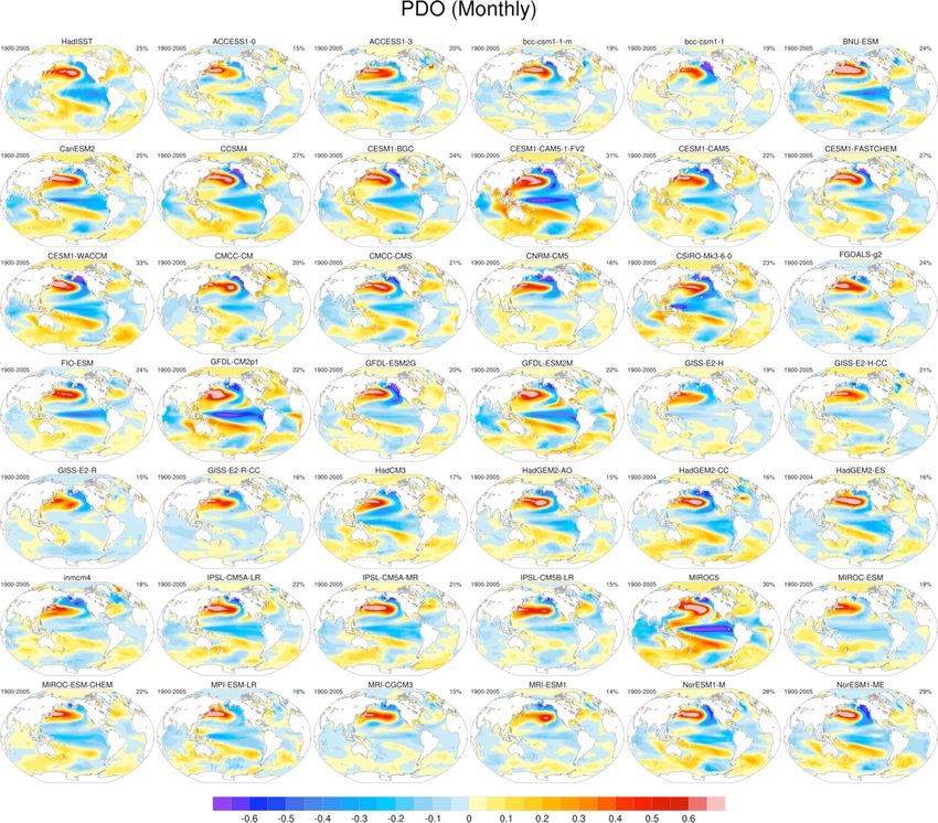
Day 3 - 2018 CESM TutorialClimate Variability Diagnostic Package
The Climate Variability Diagnostics
Package (CVDP) is the newest of the
diagnostics packages. The CVDP
calculates the major modes of
variability (AMO, PDO, NAM, etc.),
AMOC metrics, and trends amongst
other calculations.
Unlike the other diagnostics
packages, this package is run over
decades/centuries and allows
multiple simulations to be input at
once. Data from the CMIP3 or CMIP5
archives are also allowed, allowing
intercomparisons between CESM and
other models. Calculations can be
output to netCDF files for future use.
The CVDP is a component of the Earth
System Model Validation Tool (ESMValTool).
VI. Practical Lab #3: Diagnostics Packages
Day 3 - 2018 CESM TutorialClimate Variability Diagnostic Package
The CVDP website also
contains a Data Repository
where we provide CVDP
output for most of the
CMIP3 and CMIP5
simulations, as well as for
general CCSM/CESM
simulations.
http://www.cesm.ucar.edu/working_groups/CVC/cvdp/
VI. Practical Lab #3: Diagnostics Packages
Day 3 - 2018 CESM TutorialDiagnostics Packages
The diagnostics packages are available off of github, with the exception
of the CVDP which is available from the SVN repository.
The diagnostics packages were built to be flexible. Many comparisons
are possible using the options provided. Here, we have you set a few
options to compare observations to your model run. You can also use
the diagnostics to compare model runs to one another, regardless of
model version.
Typically, 10-25 year time slices of data are analyzed using the
component diagnostics. (Exception: The ocean timeseries diagnostics
are usually run on the entire simulation.) Here, you only have ~3 years
of data, so that’s what we will use.
If you wish to take these diagnostics packages back with you to your
home institution, you will need to have the netCDF operators and NCL
installed, as well as Image Magick.
VI. Practical Lab #3: Diagnostics Packages
Day 3 - 2018 CESM TutorialDiagnostics Packages
Each component diagnostics package has different requirements in terms of
the minimum amount of data required for them to run. (Ocean: 12 months,
Atmosphere, Land: 14 months, Ice: 24 months)
If you do not have the amount of data needed to run a specific diagnostics
package, there is a directory set up with 3 years of a Day 2 case here:
/glade/scratch/asphilli/archive/b.day2.1
(Path also given in test_data_location.txt file found in scripts/ directory.)
Only complete years can be analyzed by the packages, and there has to be an
additional December before the 1st analyzed year or an additional January and
February the year after the last analyzed year. If you have 14 complete years of
data you cannot set the first analyzed year to 1 and the last analyzed year to 14.
Either set the first analyzed year to 2 or the last analyzed year to 13.
Do not enter leading 0’s. example: 0012
You can usually ignore the various NCL/convert warning messages within the
log files, as frequently there are model variables missing that the packages
expect. You will know when it is an error message you should address.
VI. Practical Lab #3: Diagnostics Packages
Day 3 - 2018 CESM TutorialPractical Lab #3
Within the lab, you will have the opportunity to play with the CESM
history files that you created. There are 5 sets of diagnostics scripts, 4
NCL post-processing scripts, 7 NCL graphics creating scripts, and 2
pyNIO/pyNGL scripts. You will also be able to try out the various
software packages discussed earlier (ncview, ImageMagick, etc.).
The following slides contain information about how to run the various
scripts on cheyenne, along with exercises that you can try. It is suggested
that you first focus on running those scripts written for the model
component that you’re most interested in. For instance, if you’re an
oceanographer, try running the ocean diagnostics script, along with the
ocean post-processing script and ocean graphics NCL scripts.
Once you’ve completed running one of the diagnostics packages, take
a run at one of the other packages, or try the exercises/challenges on
the last two slides.
You are not expected to run every diagnostics package and exercise.
VI. Practical Lab #3: Diagnostics Packages
Day 3 - 2018 CESM TutorialGetting Started (Start on this slide for lab session)
To set up your environment for today’s lab:
1) You will not be logging into a specific cheyenne node, so login to
cheyenne by issuing this command: ssh –Y cheyenne.ucar.edu
2) For tcsh users: You should have a .tcshrc file already present in your
home directory. If you do not, please copy over the following file:
cp /glade/p/cesm/tutorial/tcshrc ~/.tcshrc
change to your home directory and source the file: cd; source .tcshrc
If you have an existing .tcshrc file and do not wish to overwrite it
please copy the contents of the /glade/p/cesm/tutorial/tcshrc file to
your .tcshrc file.
For bash users: See the following website:
https://github.com/NCAR/CESM_postprocessing/wiki/
yellowstone-and-cheyenne-quick-start-guide
and add the bash coding in step #1 to your .profile. You will also
need to add: PROJECT=UESM0006;export PROJECT
VI. Practical Lab #3: Diagnostics Packages
Day 3 - 2018 CESM TutorialGetting Started
3) cd to your home directory, then create a new directory named
scripts, and cd into it:
cd
mkdir scripts
cd scripts
Copy all files from my CESM_tutorial directory over to your scripts
directory, and rename hluresfile (sets NCL defaults) to .hluresfile:
cp –R /glade/u/home/asphilli/CESM_tutorial/* .
mv hluresfile ../.hluresfile
VI. Practical Lab #3: Diagnostics Packages
Day 3 - 2018 CESM TutorialRunning the Component Diagnostics
The following pages contain instructions on how to run each of the four
component diagnostics packages. Each qsub submission you make
should take on the order of ~5 minutes.
Note that the general CESM (component) diagnostics instructions are
located here:
https://github.com/NCAR/CESM_postprocessing/wiki/yellowstone-and-
cheyenne-quick-start-guide
Customized instructions for the tutorial are given over the next few
slides. You will need to change all settings that are encased in < >.
1) Set up your python environment:
cesm_pp_activate
2) Create a directory to house the CESM postprocessing code:
mkdir /glade/scratch//cesm-postprocess
VI. Practical Lab #3: Diagnostics Packages
Day 3 - 2018 CESM TutorialRunning the Component Diagnostics
3) Decide which simulation you will run the diagnostics on, either your run
or one of the two test cases specified in
~/scripts/test_data_location.txt. Then run create_postprocess to set
up your post-processing directory, and cd to that directory as follows:
create_postprocess --caseroot /glade/scratch//cesm-postprocess/
cd /glade/scratch//cesm-postprocess /
For instance, if you are running on your b.day2.1 simulation:
create_postprocess --caseroot /glade/scratch//cesm-postprocess/b.day2.1
cd /glade/scratch//cesm-postprocess /b.day2.1
Reminder: Your model data location: /glade/scratch//archive/
Note the - - syntax (not separated by a space)
VI. Practical Lab #3: Diagnostics Packages
Day 3 - 2018 CESM TutorialRunning the Component Diagnostics
4) You will now set options in various .xml files in preparation for
running. You can do the modifications by hand, or you can do them
by using the pp_config command. It is highly recommended that you
use the pp_config command as that will check that your changed
settings are valid.
The first file that needs modification is env_postprocess.xml. (Note
that if you alternatively set up your cesm-processing directory (step
3) within the archive directory of your model run, you can skip this
step as everything should be set automatically.)
Set the location of the model data:
./pp_config --set DOUT_S_ROOT=
(Example: ./pp_config --set
DOUT_S_ROOT=/glade/scratch//archive/b.day2.1)
Tell the diagnostics what kind of grids to expect. Our tutorial simulations use
1.9x2.5_gx1v7:
./pp_config --set ATM_GRID=1.9x2.5
./pp_config --set LND_GRID=1.9x2.5
./pp_config --set ICE_GRID=gx1v7
./pp_config --set OCN_GRID=gx1v7
./pp_config --set ICE_NX=320
./pp_config --set ICE_NY=384
VI. Practical Lab #3: Diagnostics Packages
Day 3 - 2018 CESM TutorialRunning the Atmospheric Diagnostics Package
Remember that the atmospheric diagnostics need at least 14 months to
run, and that you can only specify complete years. The steps to run the
atmospheric diagnostics are as follows:
1) The following commands edit settings in env_diags_atm.xml.
./pp_config --set
ATMDIAG_OUTPUT_ROOT_PATH=/glade/scratch//diagnostics-output/atm
./pp_config --set ATMDIAG_test_first_yr=
./pp_config --set ATMDIAG_test_nyrs=
2) Before the atmospheric diagnostics can be run monthly climatologies
must be calculated and written to netCDF files. To run the
atmospheric averages script:
qsub atm_averages
To monitor that status of your submission you can type qstat –u
You can check progress by checking the newest log file in
logs/. If in a log file you notice that things have gone wrong, you can
stop your submission by typing qdel
VI. Practical Lab #3: Diagnostics Packages
Day 3 - 2018 CESM TutorialRunning the Atmospheric Diagnostics Package
3) Once the averages have successfully completed (check the end of
the newest log file), you can submit the diagnostics script:
qsub atm_diagnostics
4) Again monitor the status of your submission by checking the newest
log file in the logs/ directory. Do not be concerned by various error
messages (like convert error messages) from individual scripts in the
log files. If the submission completed successfully the log file will end
with “Successfully completed generating atmosphere diagnostics”.
5) Once the diagnostics are complete, cd to the location of the
diagnostics:
cd /glade/scratch//diagnostics-output/atm/diag/-obs.-
y0 = first year of analysis, y1 = last year of analysis
and open the index.html in firefox to examine the output:
firefox index.html &
For more information about the AMWG Diagnostics Package:
http://www.cesm.ucar.edu/working_groups/Atmosphere/amwg-diagnostics-package/
VI. Practical Lab #3: Diagnostics Packages
VI. Practical Lab #3 Day 3 - 2018 CESM TutorialRunning the Land Diagnostics Package
Remember that the land diagnostics need at least 14 months to run , and
that you can only specify complete years. The steps to run the land
diagnostics are as follows:
1) The following commands edit settings in env_diags_lnd.xml.
./pp_config --set
LNDDIAG_OUTPUT_ROOT_PATH=/glade/scratch//diagnostics-output/lnd
./pp_config --set LNDDIAG_clim_first_yr_1=
./pp_config --set LNDDIAG_clim_num_yrs_1=
./pp_config --set LNDDIAG_trends_first_yr_1=
./pp_config --set LNDDIAG_trends_num_yrs_1=
2) Before the land diagnostics can be run monthly climatologies must
be calculated and written to netCDF files. To run the land averages
script: qsub lnd_averages
To monitor that status of your submission you can type qstat –u
You can check progress by checking the newest log file
in logs/. If in a log file you notice that things have gone wrong, you
can stop your submission by typing qdel
VI. Practical Lab #3: Diagnostics Packages
Day 3 - 2018 CESM TutorialRunning the Land Diagnostics Package
3) Once the averages have successfully completed (check the end of
the newest log file), you can submit the diagnostics script:
qsub lnd_diagnostics
4) Again monitor the status of your submission by checking the newest
log file in the logs/ directory. Do not be concerned by various error
messages (like convert error messages) from individual scripts in the
log files. If the submission completed successfully the log file will end
with “Successfully completed generating land diagnostics”.
5) Once the diagnostics are complete, cd to the location of the
diagnostics:
cd /glade/scratch//diagnostics-output/lnd/diag/-obs._
and open the setsIndex.html in firefox to examine the output:
firefox setsIndex.html &
For more information about the LMWG Diagnostics Package:
http://www.cesm.ucar.edu/models/cesm1.2/clm/clm_diagpackage.html
VI. Practical Lab #3: Diagnostics Packages
Day 3 - 2018 CESM TutorialRunning the Ocean Diagnostics Package
Historically the ocean diagnostics package consisted of three separate
sets of scripts, one that compared a model run to observations, one that
compared a model run to another model run, and one that calculated
timeseries. Here, you will compare your simulation to observations and
calculate ocean timeseries. Remember that the ocean diagnostics need
at least 12 months to run, and that you can only specify complete years.
The steps to run the ocean diagnostics are as follows:
1) The following commands edit settings in env_diags_ocn.xml.
./pp_config --set OCNDIAG_YEAR0=
./pp_config --set OCNDIAG_YEAR1=
./pp_config --set OCNDIAG_TSERIES_YEAR0=
./pp_config --set OCNDIAG_TSERIES_YEAR1=
./pp_config --set OCNDIAG_TAVGDIR=/glade/scratch//
diagnostics-output/ocn/climo/tavg.$OCNDIAG_YEAR0.$OCNDIAG_YEAR1
./pp_config --set OCNDIAG_WORKDIR=/glade/scratch//
diagnostics-output/ocn/diag/.$OCNDIAG_YEAR0.$OCNDIAG_YEAR1
If the latter two commands result in an error message, edit the env_diags_ocn.xml file
manually to set those two directory paths.
VI. Practical Lab #3: Diagnostics Packages
Day 3 - 2018 CESM TutorialRunning the Ocean Diagnostics Package
2) Before the ocean diagnostics can be run monthly climatologies must
be calculated and written to netCDF files. To run the ocean averages
script: qsub ocn_averages
To monitor that status of your submission you can type qstat –u
You can check progress by checking the newest log file
in logs/. If in a log file you notice that things have gone wrong, you
can stop your submission by typing qdel
3) Once the averages have successfully completed (check the end of
the newest log file), you can submit the diagnostics script:
qsub ocn_diagnostics
4) Again monitor the status of your submission by checking the newest
log file in the logs/ directory. Do not be concerned by various error
messages (like convert error messages) from individual scripts in the
log files. If the submission completed successfully the log file will end
with “Successfully completed generating ocean diagnostics …..”.
VI. Practical Lab #3: Diagnostics Packages
Day 3 - 2018 CESM TutorialRunning the Ocean Diagnostics Package
5) Once the diagnostics are complete, cd to the location
of the diagnostics:
cd /glade/scratch//diagnostics-output/ocn/diag/.-
and open the index.html in firefox to examine the output:
firefox index.html &
VI. Practical Lab #3: Diagnostics Packages
Day 3 - 2018 CESM TutorialRunning the Ice Diagnostics Package
Remember that the ice diagnostics need at least 24 months to run , and
that you can only specify complete years. The steps to run the ice
diagnostics are as follows:
1) The following commands edit settings in env_diags_ice.xml.
./pp_config --set ICEDIAG_BEGYR_CONT=
./pp_config --set ICEDIAG_ENDYR_CONT=
./pp_config --set ICEDIAG_YRS_TO_AVG =
./pp_config --set ICEDIAG_PATH_CLIMO_CONT=/glade/scratch//diagnostics-
output/ice/climo/$ICEDIAG_CASE_TO_CONT/
./pp_config --set ICEDIAG_DIAG_ROOT=/glade/scratch//diagnostics-
output/ice/diag/$ICEDIAG_CASE_TO_CONT/
If the latter two commands result in an error message, edit the
env_diags_ice.xml file manually to set those two directory paths.
VI. Practical Lab #3: Diagnostics Packages
Day 3 - 2018 CESM TutorialRunning the Ice Diagnostics Package
2) Before the ice diagnostics can be run monthly climatologies must be
calculated and written to netCDF files. To run the ice averages script:
qsub ice_averages
To monitor that status of your submission you can type qstat –u
You can check progress by checking the newest log file in
logs/. If in a log file you notice that things have gone wrong, you can
stop your submission by typing qdel
3) Once the averages have successfully completed (check the end of
the newest log file), you can submit the diagnostics script:
qsub ice_diagnostics
VI. Practical Lab #3: Diagnostics Packages
Day 3 - 2018 CESM TutorialRunning the Ice Diagnostics Package
4) Again monitor the status of your submission by checking the newest
log file in the logs/ directory. Do not be concerned by various error
messages (like convert error messages) from individual scripts in the
log files. If the submission completed successfully the log file will end
with “Successfully completed generating ice diagnostics”.
5) Once the diagnostics are complete, cd to the location of the
diagnostics:
cd /glade/scratch//diagnostics-output/ice/diag//
-obs/yrs-
and open the index.html in firefox to examine the output:
firefox index.html &
VI. Practical Lab #3: Diagnostics Packages
Day 3 - 2018 CESM TutorialClimate Variability Diagnostics Package
The CVDP is different from the component diagnostic packages, in that the
CVDP is run on timeseries/post-processed data (only), and can be run on non-
CESM data. Input models do not need to be on the same grid. The CVDP can
also be run on 2+ simulations at once. Entire simulations (spanning 100’s of
years) can be passed into the package, but note that your ~5yr tutorial
simulations are too short to put in the CVDP.
All input file names must end with the standard CMIP5 file naming syntax
“YYYYMM-YYYYMM.nc”. Soft links can be used to meet this requirement.
The CVDP reads in 8 variables: aice, MOC, PRECC, PRECL, PSL, SNOWDP,
TREFHT, and TS. (CMIP names: sic, stfmmc/msftmyz, pr, psl, snd, tas,ts)
Three scripts need to be set up to run the CVDP:
namelist (lists the location of model run data to be analyzed)
namelist_obs (specified which observational datasets to use)
driver.ncl (sets CVDP options)
For the lab session, you will have the chance to run the CVDP on three
simulations from the CESM1 Large Ensemble Project.
https://www.cesm.ucar.edu/projects/community-projects/LENS
VI. Practical Lab #3: Diagnostics Packages
Day 3 - 2018 CESM TutorialClimate Variability Diagnostics Package
1) Login to Cheyenne, then jump onto a processing machine:
ssh –Y cheyenne.ucar.edu
execdav --account=UESM0006 (=log on to geyser or caldera)
Note: If X11 forwarding is not working on caldera/geyser, open a 2nd terminal
window on cheyenne, and use this second window for editing/viewing.
2) cd to your scripts directory, then into CVDP:
cd ~/scripts/CVDP
3) Open up the namelist using your favorite text editor:
gedit namelist (or use xemacs, vi, etc.)
The format of each row in namelist is as follows:
Run Name | Path to all data for a simulation | Analysis start year | Analysis end year
Modify each of the three rows so that the analysis start and end years
are specified as 1979 and 2015. (They can be different though.) Note
that “ | “ serves as the delimiter.
VI. Practical Lab #3: Diagnostics Packages
Day 3 - 2018 CESM TutorialClimate Variability Diagnostics Package
4) Open up the namelist_obs:
gedit namelist_obs (or use xemacs, vi, etc.)
The format of each row in namelist_obs is as follows:
Variable | Obs Name | Path to obs dataset | Analysis start year | Analysis end year
namelist_obs is already set appropriately, so no changes need to be
made. These datasets are not distributed with the CVDP, but can be
downloaded online. Note that MOC, SNOWDP, aice_nh and aice_sh
do not have observational datasets and are not listed.
5) Open up the driver.ncl:
gedit driver.ncl (or use xemacs, vi, etc.)
Modify:
line 7 replace user with your logname
line 18 change “False” to “True” to output calculations to netCDF
VI. Practical Lab #3: Diagnostics Packages
Day 3 - 2018 CESM TutorialClimate Variability Diagnostics Package
6) Run the CVDP on one of cheyenne’s compute nodes by submitting
driver.ncl:
ncl driver.ncl
7) Once the CVDP is complete (~20 mins), cd to the outdir specified in
driver.ncl, fire up a firefox window, and open up the index.html file:
cd /glade/scratch//CVDP
firefox index.html &
VI. Practical Lab #3: Diagnostics Packages
Day 3 - 2018 CESM TutorialNCL post-processing scripts
All 4 post-processing scripts are quite similar, and are located in your
scripts directory. To list them, type: ls *create* . If these scripts are
used for runs other than the tutorial runs, note that the created netCDF
files may get quite large (especially pop files). This can be mitigated by
setting concat and concat_rm = False.
To set up the post-processing scripts, alter lines 7-15 (7-17 for atm).
There are comments to the right of each line explaining what each line
does.
To run the atm script (for example), type the following:
ncl atm.create_timeseries.ncl
All 4 scripts will write the post-processed data to work_dir (set at top of
each script)/processed/. Once the post-processing is complete, we
can use the new files in our NCL graphics scripts, or view them via
ncview.
VI. Practical Lab #3: Post-processing scripts
Day 3 - 2018 CESM TutorialNCL Graphics Scripts
These scripts are set up so that they can read either raw history files from
your archive directory (lnd,ice,ocn history files) or the post-processed files
after they’ve been created by the NCL post-processing scripts.
You will need to modify the user defined file inputs at the top to point to your
data files, either your raw history files or your newly created post-processed
files. Once the files are modified, to execute the scripts, simply type (for
example):
ncl atm_latlon.ncl . To see the script output use gv: gv atm_latlon.ps
There are 7 NCL graphics scripts available for you to run:
atm_latlon.ncl atm_nino34_ts.ncl ice_south.ncl
ice_north.ncl lnd_latlon.ncl ocn_latlon.ncl
ocn_vectors.ncl
The ocn_vectors.ncl allows you to compare one ocean history file to another,
and is more complicated (you can modify the first 50 lines) than the other 6
scripts. To run them, simply set the options at the top of the script.
VI. Practical Lab #3: Graphics Scripts
Day 3 - 2018 CESM TutorialpyNIO/pyNGL Graphics Scripts
Two of the NCL graphics scripts (ice_south/ice_north) have been transcribed
to python and use pyNIO and pyNGL. Both use history files.
You will need to modify the user defined file inputs at the top to point to your
history file. You will also have to login to geyser and load the python2 module
and pyNIO/pyNGL libraries.
execgy ; log into geyser from cheyenne. If this repeatedly fails, logout of
; cheyenne and then back in, and try the execgy command again
module load python/2.7.14 ; load python v2.7.14
ncar_pylib ; load NCAR python package library
Once the environment is set, to execute the scripts simply type (for example):
python ice_south.py
To see the script output use display:
display ice_south.png
Scripts courtesy of Dave Bailey
VI. Practical Lab #3: Graphics Scripts
Day 3 - 2018 CESM TutorialExercises
1) Use ncdump to examine one of the model history files. Find a
variable you’ve never heard of, then open up the same file using
ncview, and plot that variable.
2) Modify one of the NCL scripts to plot a different variable.
3) Use the netCDF operators to difference two files. Plot various fields
from the difference netCDF file using ncview.
4) Convert the output from one of the NCL scripts from .ps to .jpg, and
crop out the white space. Import the image into Powerpoint.
5) Use the netCDF operators to concatenate sea level pressure and
the variable date from all the monthly atmospheric history files
(.h0.) from one of your model simulations into one file.
6) Same as 5), but only do this for the Northern Hemisphere.
7) Same as 6), but don’t append the global history file attribute.
VI. Practical Lab #3: Exercises
Day 3 - 2018 CESM TutorialChallenges
1) Modify one of the NCL scripts to alter the look of the plot. Use the
NCL website’s Examples page to assist.
2) Add a variable or 3 to one of the post-processing scripts, then
modify one of the NCL scripts to plot one of the new variables.
3) Use the atmospheric diagnostics package to compare 2
simulations to one another. (Use one or two of the model
simulations provided in test_data_location.txt)
4) Use the ocean diagnostics package to compare 2 simulations to
one another.
VI. Practical Lab #3: Challenges
Day 3 - 2018 CESM TutorialYou can also read