AI AND MACHINE LEARNING A QUICK INTRODUCTION - Methods in experimental particle physics Roma 13.6.2019 S. Giagu
←
→
Page content transcription
If your browser does not render page correctly, please read the page content below
AI AND MACHINE LEARNING
A QUICK INTRODUCTION …
Methods in experimental particle physics
Roma 13.6.2019
S. Giagu
REFERENCES AND FURTHER READING …
•   Machine Learning and Deep Learning:
    •   Pattern Classification: R.O. Duda, P.R. Hart, D.G. Stork, (2nd ed.) J.Wiley&Sons
    •   Stat. Pattern Recognition: A. Webb, (3rd ed.), J.Wiley&Sons
    •   Decision Forests for Computer Visions and Medical Image Analysis: A.Criminisi, J.Shotton, Springer
    •   Deep Learning: I.Goodfellow, Y.Bengio, A.Courville, The MIT Press

•   Artificial Intelligence (introductive):
    •   Artificial Intelligence: A Modern Approach: P.Norvig. (free on web)
    •   Life 3.0 – Being Human in the Age of Artificial Intelligence: M. Tegmark
    •   Fundamental Algorithms: 1 (Artificial Intelligence for Humans): J.Heaton (more advanced)

•   Tools/frameworks:
    •   Keras & TensorFlow: https://keras.io, https://www.tensorflow.org
    •   XGBoost: https://xgboost.ai
    •   Scikit-learn: https://scikit-learn.org/stable/
    •   PyTorch: https://pytorch.org

                                                                                                             2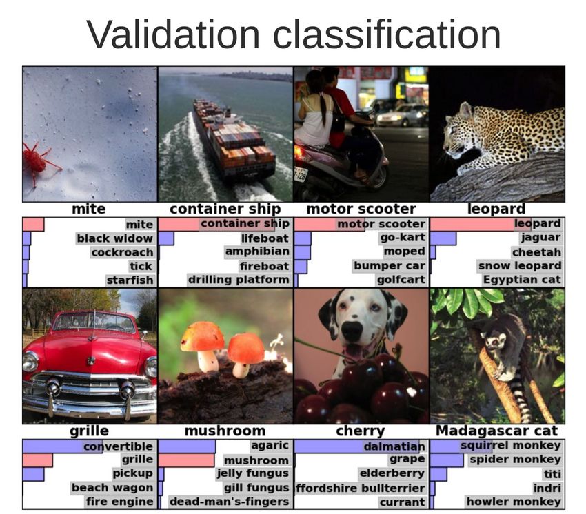
INTRODUCTION
•   What Machine Learning means?

    •   ML is part of a larger research filed called
        Artificial Intelligence (AI) focused in the
        attempt to automatize intellectual tasks
        that are generally performed by humans

                                                       3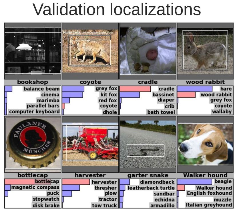
AI
    •   the AI concept and the study and development of ML algorithms used in AI systems
        started in the early 50’, but it is only in the last ~10 years that AI applications are
        spreading exponentially in the society outside the basic and accademico research field

•   This acceleration motivated by three parallel developments:

        •   better algorithms (Machine & Deep Learning)

        •   higher computing power (GPUs/TPUs/HPCs)

        •   ability of the technological and industrial sectors to record and make accessible
            huge amounts of data/information (grid, clouds)

                                                                                                  4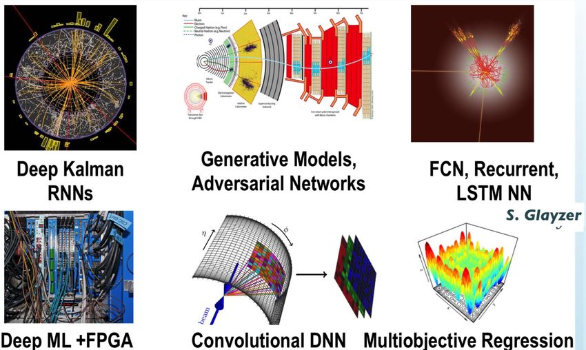
MACHINE LEARNING
 •   Original definition (Arthur Samuel, 1959):

     Computational methods (algorithms) able to emulate the typical human,
     or animal, behaviour of learning based on the experience (i.e. learning
     from examples), w/o being explicitly programmed

     ML algorithms are meant to solve that class of problems (like image or
     language recognition) that cannot be simply described with a set of
     formal mathematical rules (equations) and so too complex to be resolved
     by a traditional computational algorithm

                                                                               5
MACHINE LEARNING VS TRADITIONAL COMPUTATION

  •   Traditional computation (symbolic AI): the programmer (human) design and load a
      set of rules (program) in the processor together a set of data that are analysed
      accordingly the set of rules to output an answer to the problem we want to solve

                           D ATA

                                        TRADITIONAL
                                                        ANSWERS
                                       PROGRAMMING

                           RULES
                        (PROGRAM)

                                                                                         6
MACHINE LEARNING VS TRADITIONAL COMPUTATION

  •   ML: the programmer present to the processor both the data set and the set of
      answers expected for that data set. The algorithm output a set of rules that can then
      applied to indipendenti datasets to get the original answers

                                   D ATA
                                (EXAMPLES)

                                                       MACHINE
                                                                             RULES
                                                       LEARNING

                                 ANSWERS

      a ML system is “trained” not programmed …
      •   is feed with a set of relevant examples gli vengono presentati un certo numero di esempi significativi
      •   try to find statistical structures in these examples (we assume these structures exist), that eventually
          will allow the algorithm to learn the rules needed to learn to perform a certain task
                                                                                                                     7
A MODERN DEFINITION (MITCHELL, 1998)

• an algorithm is said to learn from experience (E) with respect to some class of
  tasks (T) and a performance measure (P), if its performance at tasks in T, as
  measured by P, improves with experience E

• Task T: are described in terms of how the ML algorithm should process the example E
  • typical ML tasks:
    • classification (f:Rn→{1,…,k}), regression (f:Rn→Rm), images segmentation,
      transcription (ex. OCR), conversion of sequences of symbols (automatic translation),
      anomaly detection, synthesis/sampling (es. generators), de-noising, …

                                                                                             8
• Example/Experience E:
 • represent the set of empirical information from which the algorithm learn
    • training set (i.e. the data)
    • prior knowledge: invariants, correlations, …

• Performance measure P: to evaluate the abilities of a machine learning algorithm, we must
  design a quantitative measure of its performance. Usually this performance measure P is
  specific to the task T being carried out by the system
  • accuracy (fraction fo examples for which the algorithm produce the correct output),
     error rate, statistical costs, ROC, AUC, …
  • must be always evaluated in a statistically independent data set (test sample)

                                                                                            9
LEARNING PARADIGMS
• Learning algorithms can be divided in different categories that defines which kind of experience is
 permitted during the training process

                                                                                                       ∈B
                                                                                             x2               x
• supervised learning (i.e. there is a teacher):                                                            x x x
  - for each example of the training set is provided the true answer (for example the             ∈A         x x
    corresponding class) called label
                                                                                                    x x
  - Typical target of the training process: to minimise the classification error or the            x x
    accuracy
                                                                                                                  x1
                                                                                                        CB
• unsupervised (or better: auto-supervised) learning:                                        x2               x
                                                                                                            x x x
  - no explicit information on the true answer for the training set examples is given                        x x
  - typical target of the training process: create groups / clusters of the input objects,
                                                                                                    x x
    generally on the base of similarity criteria
                                                                                                   x x
                                                                                                             CA
                                                                                                                  x1
                                                                                                                       10
UNSUPERVISED LEARNING ALGORITHM EXAMPLE: GOOGLE NEWS
11• Reinforcement learning:
inspired by behavioral psychology: is not used a fixed set of examples/experiences, but the
algorithms adapts to teh ambient with which interacts via a continuous feedback between system
and examples and through the distribution of a sort of reward (reinforce) that acts on the
performance measure P
Supervised ConvNet
Associate a label
Solve the complex problem of relating to an image
instantaneous actions with the effect that they
may produce at a later time
example: to maximise the score in a game that
develop over multiple moves Convolutional
agent
Maps a state to the best
possibile action
12ML: LEARNIGN PARADIGMS AND TASKS
13AI/ML APPLICATIONS EXAMPLES
Face/Object Detection:
- static: ex. facebook photos
- real time: cameras, autonomous driving systems
- experience: portion of images
- task: face or not-face
Medical Image Detection e Segmentation:
- experience: images (list of pixels)
- task: identify different biological tissues,
disomogeneities …
Voice recognition:
- experience: acoustical signals
- task: identify phonemes
ma-chin-le-ar-nin-g
14AI/ML APPLICATIONS EXAMPLES
Autonomous drive
Search engines
SPAM detection
Autonomous Drones
15APPLICATIONS IN Adversarial CNN to identify phase
transitions in matter
PHYSICS
high energy physics applications
credits: D.Glayzer
And many more … 16CONCEPTUAL SCHEME OF THE SIMPLEST CLASSIFICATION SYSTEM
• Given the description of an object that can belong to N possible classes, task for
the system is to assign the object to one of the classes (o to assigna probability
Schema ideale di un
to each class) by using the knowledge base build during the training phase
sistema di riconoscimento
SENSOR:
Sistema di the features are used as
acquisizione e input to a recognition
descrizione algorithm that on the base of
classe 1 such features classifies the
CLASSIFICATORE:
object
classe 2
Sistema di
riconoscimento ?
classe N
FEATURE EXTRACTOR:
descrizione
oggetto da dell=oggetto
riconoscere
The feature estractor present to the recongition F. Tortorella © 2005
Teoria e Tecniche di Pattern Recognition
system a description, i.e. a set of measures (features) Università degli Studi
Sistemi per il P.R. 2
that characterise the object to be recognised
di Cassino
17Rappresentazione
descrizione e
descrizione
RAPPRESENTATIONS
• 16x16=256 pixel represent the object
" 16x16=256 pixel rappresentano l9oggetto
" •16x16=256 pixel
From these pixels we rappresentano l9oggetto
can extract a set of measures (typically with a smaller
"dimension
da questi si#possono
wrt the ricavare
of pixels) that unobject
describe the insieme di misure
(ex. Ratio between on/
" da questiarea
off pixels, si possono ricavare
or perimeter un insieme
of the clusters, di misure
…): features
sintetiche (di solito in numero molto minore) che
sintetiche (di solito in numero molto minore) che
descrivono
descrivono l9oggetto l9oggetto
each object is then represented by a
"" Ad
Ad ogni
ogni oggetto
oggetto corrisponde
corrisponde
feature vector, that corresponds to a
una descrizione in
una descrizione in forma di
point in the feature space forma di
vettore di features (feature
vettore di features (feature
vector) che corrisponde ad
vector) che corrisponde
un punto in uno spazio delle ad
un punto in uno spazio
features (feature space) delle
Teoria e Tecniche di Pattern Recognition
F. Tortorella © 2005 18CHOICE OF FEATURES
• thechoice of the best representation of the data is one of the most crucial and important aspects of a ML
algorithm
example: identification of rural and
urban areas in satellite images based
on spectral properties of the images
19LERN THE DATA REPRESENTATION
in first generation (classic ML): the feature set were build and
chosen by the operator on the base of prior knowledge of the
problem itself
• human: identify best features
• algorirthm: identify the best mapping between features and output
second generation ML: Representation Learning
• the algorithm scope is expanded by performing also the task to find in
an automatic way a better representation of the data with respect to
the one available with the input features
20DEEP LEARNING (DL)
• the traditional ML algorithms were not very “cerative” in finding better
representations
• basically they just searched the best possible transformation in a predefined set of
operations called ”hypothesis space” of the algorithm. Search guided by the training
examples
• The Deep Learning evolution solve this limitation by organising ideas and concepts in
a hierarchical way and building new complex representations based on simpler ones
• example: a person face can be presente by combining simpler features: eyes, mouth,
hears …, that can be represented in trun by combining basic features: edges,
contours, lines, …
• DL == HIERARCHICAL REPRESENTATION LEARNING
Extremely powerful, but requires huge training sets
and a lot of computing power …
21AUTOENCODER: A BASIC EXAMPLE OF REPRESENTATION LEARNING
• non-supervised algorithm that try to identify common and fondamentali characteristic in the input data
• combines and encoder that converts input data in a different representation, with a decoder that
converts the new representation back to the original input
• trained to output something as close as possible to the input (learn the identity function)
ENCODER DECODER
• “trivial” unless to constrain the network to have the hidden
input representation with a smallare dimension of the input/output
v(5) • in such case the network build (learn) “compressed”
representations of the input features: x∈R5→z∈R3→⋯
bottleneck output = input
22DL: INTUITIVE EXPLANATION …
tt is like to solve the Rubik
goal of the rappresentation-learning algorithm is to find the best transformation
in the DL this is implemented by a sequence of simpler transformations (in the
specific example rotations in the 3D space)
Sequence of roations
∈ Rubik’s group
23DECISION BOUNDARIES Scelta delle features
• let’s assume that we have found that the two best features for our classification task are: length e lightness
• which one we should use for the classification? Which threshold?
• to decide this we make use of the traing set examples
Classification rule: if x > x*:
else:
object ∈ class A
objetc ∈ class B
Scelta delle features
La feature scelta non è molto discriminante. C>è una certa d
media, ma non tale da separare nettamente le due classi.
F.
Teoria e Tecniche di Pattern Recognition
U
Sistemi per il P.R. 8 di
the threshold x* is chosen in order to optimize an appropriate performance
measure
example: accuracy, probability of misclassificantion, statistical risk …
La nuova feature scelta
decision permette una distinzione mi
boundary 24DECISION BOUNDARIES
• to improve P a better strategy woudl be to use more than one feature at the same time
• The classification problem becomes the problem to find the best partition of the feature space, so that the
classification error is the smallest one
decision regions decision boundary
• Simplest choice: linear boundary (linear classifier)
Decision rule:
if w0 + w1∙x1 + w2∙x2 > 0: object ∈ class A
else: object ∈ class B
25COMPLEX DECISION BOUNDARIES …
• question: it is possible to get rid of all errors with a complex decision boundary?
example: this boundary correctly clasify all the events of
the trining set
PROBLEM: this way we are NOT guarantee a good
performance of the algorithm when applied to events from
independent samples wrt the training set (overfitting)
• The training set has finite dimension and the decision boundary is sensitive to the statistical
fluctuation in the training set
• This aspect is called generalisation problem, and sis the crucial aspect in the design and
training of any ML algorithm! 26Minimizzazione
VAPNIK THEORY del Rischio
Strutturale
bias-variance tradeoff: if we use a more complex model we pay a price of a larger variance …
Optimal
R(f)
Minimizzazione del
underfitting Rischio
Strutturale
Ci sono due approcci costruttivi per overfitting
minimizzare il termine R (f)
s
h(log(2 S /h) 1) log( /4)
R S (f)
S
VC dimension: h
1. Mantenere fisso il termine di confidenza
possible (scegliendo una struttura appropriata del Shallow Neural Networks
classificatore) e minimizzare il rischio empirico.
strategies 2. Mantenere fisso il rischio empirico (p.es. uguale
Teoria e Tecniche di Pattern Recognition
SupportF. Vector
Tortorella ©Machines
2005
27
a zero) e minimizzare il termine di confidenza. Università degli StudiGENERALISATION PROBLEM
• at the end the choice of the decision boundary ia a trade off between:
-Performance of the classifier on the training-set
-Generalisation capacity of the classifier on the validation-set
• it is always preferable to accept a certain margin of error on the trining set if this allows to a
better generalisation of the algorithm
example: a decision boundary
with good performance and good
generalisation capacity
28ARTIFICIAL NEURAL NETWORKS
the most popular approach to machine and deep learning to date
an ANN is a mathematical model based on similarity with biologica neural networks:
based on an interconnected group of identical units (neurons)
process input information accordino to a connexionist computational
approach: → collective actions performed in parallel by simple
processing units (neurons)
behave as anadaptive system: structure dynamically modified during the
learning phase based on a set of examples that flow through the
network during the training step
non linear response obtained by non linear activation functions used as output of each neuron
hierarchic representation learning obtained by implementing complex architectures with multiple layers of
connected neurons (deep-NN)
29ARTIFICIAL NEURONIlMODEL
modello di neurone artificiale
di(1943)
Modello di McCulloch-Pitts McCulloch-Pitts (1943)
/ Rosenblatt (1962) F. Tortorella © 2005
Teoria e Tecniche di Pattern Recognition
Università degli Studi
Reti Neurali 12 di Cassino
Caratteristiche:
TLU:
C I segnali sono binari (xi=0/1)
Threshold binary signals (xi = 0,1)
Logic C La funzione di attivazione è
Unit synaptic
definita come: function:
n
a wi xi
i 1
C LLuscita è definita in base
activation function (i.e. output):
2 classi linearmente separabili
alla regola:
1 if a
y
Con una TLU è0possibile
if a
risolvere i problemi in cui © 2005
F. Tortorella
Teoria e Tecniche di Pattern Recognition
Reti Neurali 11
le classi siano Università degli Studi
di Cassino
linearmente separabili.
with a TLU it is possible to solve problems with linearly separable classes:
E se le classi sono
più di 2?
6 30Regioni di decisione
COMPLEX SEPARATION REGIONS
delle reti neurali
Struttura Regioni di decisione Forma generale
Semispazi delimitati da
iperpiani
Regioni convesse
Regioni di forma
arbitraria
F. Tortorella © 2005
Teoria e Tecniche di Pattern Recognition
Università degli Studi
Universal ApproximationRetiTheorem
Neurali 50 di Cassino
a feed-forward network with a single hidden layer containing a finite number of neurons
can approximate continuous functions on compact subsets of Rn, under mild assumptions
on the activation functio
NOTE: the theorem does not say anything on the effective possibility to learn in an easy
way the parameters of the network! 31SIMPLEST NN EXAMPLE: XOR GATE
_ _ MLP (sigmoid)
(A·B)+(A·B)
1
1
A 0.5
0 -2
0
B 0.5
1
1
TLU
out = θ(∑wixi) first neurone secondo neurone 32ANN: INTERPRETATION AS NON LINEAR MAPPING
• A NN can be thought as an algorithm that learn two tasks at the same time:
THIS MODULE LEARN A (NON LINEAR) MAPPING
OF THE INPUT THIS MODULE LEARN A CLASSIFIER
(LINEAR IN CASE OF A PERCEPTRON)
original space: NN: finds the non linear mapping
non linearly separable patterns x: y=Φ(x) in 3-dimensional space (three
hidden nodes) in which the patterns are
linearly separable
NN: finds the non linear mapping y=Φ(x) in
2-dimensional space (two hidden nodes) which the
patterns are “almost” linearly separable …
33FEED-FORWARD ANN Struttura della rete
(feed forward compl. connessa)
hidden layer
the most used ANN have a Feed-Forward multilayer structure:
feature vector
neurons organised in layers: input, hidden-1, ... , hidden-K, output output 1
output 2
only connections from a given layer to the next following one are allowed
output layer
input layer
F. Tortorella © 2005
Teoria e Tecniche di Pattern Recognition
Università degli Studi
Definizione della rete
Reti Neurali 19 di Cassino
1 input layer k hidden layers 1 output layer
Ogni nodo è strutturato come:
Nodo 1 1 ... 1
10
aj ... ... ...
nodo j j Livello k
Nvar discriminating input
f (aj) variables i j Mk
wji
... ...
Per il momento, non i Livello k-1
facciamo ipotesi su f (.)
activation function (or output function) N M1
F. Tortorella © 2005
Teoria e Tecniche di Pattern Recognition
Università degli Studi
34
Reti Neurali 20 di Cassino
Feed-forward Multilayer PerceptronRESPONSE FUNCTION
behaviour of the NN determined by:
topological structure of the neurons (architecture)
Weights associated to each connection
response function of each neutron to the input data
Response function ρ:
maps the input of the neuro n:x(k-1)1,…,x(k-1)n to the output x(k)j
normally divided in two parts: synaptic function k:Rn→R and the neural activation function A:R→R: ρ = k•A
1 input layer k hidden layers 1 output layer A
1 1
... 1
2 output classes
(signal and background)
... ... ...
Nvar discriminating
input variables i j Mk
.. ..
. .
x
N M1
⌅xlinear: x Lineare
⌅
⌅
(“Activation” function) ⇤ sigmoid:
1 1/(1+e x)
Sigmoide
with: A:x 1+e kx
Tanh(x)
e x
e x
⌅
⌅ T anh
⇥ ReLU:
⌅ max(0,x)
e x +e x
2
x /2)
esoftplus: log(1+e
Radialex) 35TRAINING
The training of the NN consists in adjusting the weights (and the other hyperparameters) according to a given
loss function in order to optimise the performance of the algorithm wrt a specific task
most used technique: Back-propagation
Output for an ANN with:
- a single hidden layer with A: tanh
- an output layer with A: linear nh: number of hidden layer neurons
nvar: number of input layer neurons
nh nh n
⇥
⇤ (2) (2)
⇤ ⇤ var
(1) (2)
yAN N = xj wj1 = tanh xi wij wj1
j=1 j=1 i=1
weight associated to the link weight associated to the link between
between j-th neuron of the the i-th neuron of the input layer and
hidden layer and the output the j-th neuron of the hidden layer
neutron
36TRAINING
during the training N examples are presented to the NN: xa (a=1,..,N)
for each event the output yANN(a) is computed and compared with the expected target Ya∈{0,1} (0 class 2, 1 class
1 as example for a 2-class classification algorithm)
A loss function is defined in order to measure the distance between yANN(a) e Ya:
N N
1
(x1 , ..., xN |w) = a (xa |w) = (yANN (a) Ya ) MSE
2
a=1 a=1
2
and the weight vector is chosen as the one that minimise the error Δ
Minimisation obtained with the GD/SGD …
w ( +1)
=w ( )
⇥w
37BACK-PROPAGATION
• the training happens in two phases:
• Forward phase: the weights are fixed and the input vector is propagated layer by layer up to
the output neurons (function signal)
• Backward phase: the error Δ obtained by comparing output with target is propagated
backward, again layer by layer (error signal)
• every neuron (hidden or output) receive and compare the functioned error
signals
• the back-propagation consists in a simplification of the gradient descent obtained
by recursively applying the chain rule of derivatives
38LEARNING CURVES
• at the start of the training phase the error on the training set is typically large
• with the iterations (epochs) the error tend to decrease until it reach a plateau value that depends on:
• training set size
• number of weights of the NN
• initial value of the weights
• training progress is visualizedTerminazione
with the learnign curve (error vs epochs)
• as usual multiple datasets (ordell-apprendimento
cross validation) are needed to train the NN, decide the architecture, decide the stop
criterion, and evaluate the final performances … etc..
E/n terminazione
dell-apprendimento
test validation
Teoria e Tecniche di Pattern Recognition
F. Tortorella © 2005
Università degli Studi
39DEEP LEARNING AND ANN
the different transformation/representation layers have a natural and intuitive implementation in
multilayer neural-networks:
each layer implements a transformation of the input coming
from the preceding layer
by using a sufficiently large number of hidden layers it is possible
to learn extremely complex representations and to eliminate
from the process irrilevante variations
• example: image → array of raw pixels
• first layer: find presence/absence of strong tonal
Variations in specific points of the image (edges)
• second layer: combines edges to find patterns like
corners, contours
• third layer: combines the previous patterns in complex
objects (like faces, heads, …) that can be used to
classify the content of the image …
40DEEP ARCHITECTURE OF THE BRAIN - we organise ideas and concept in hierarchical way - first we learn simple concepts, then we compose them to represent more abstract concepts - the DL try to emulate this behaviour … 41
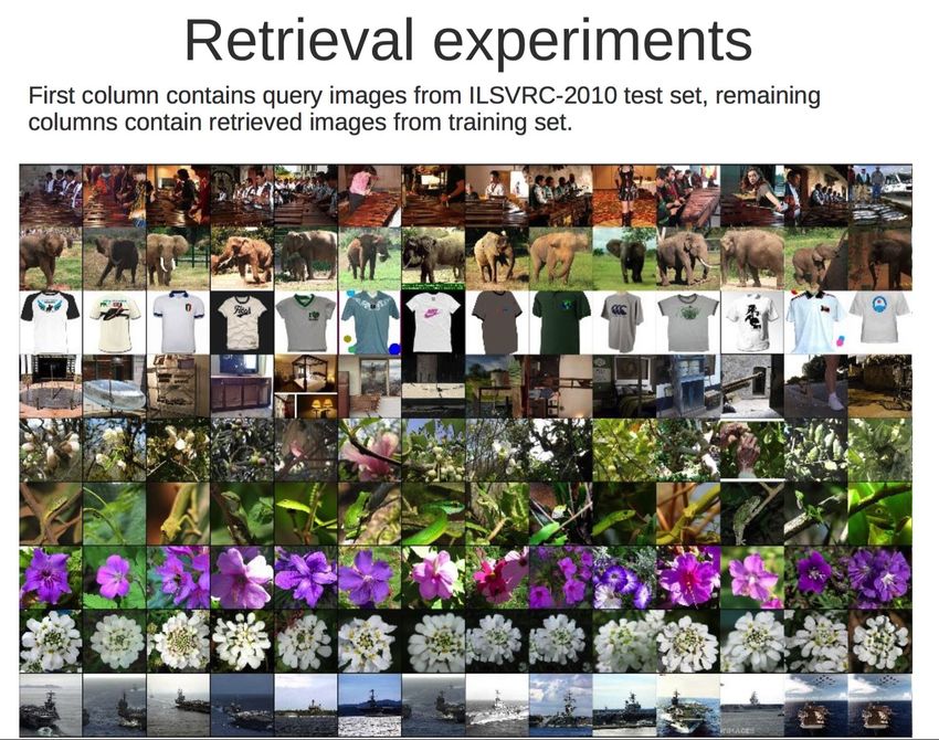
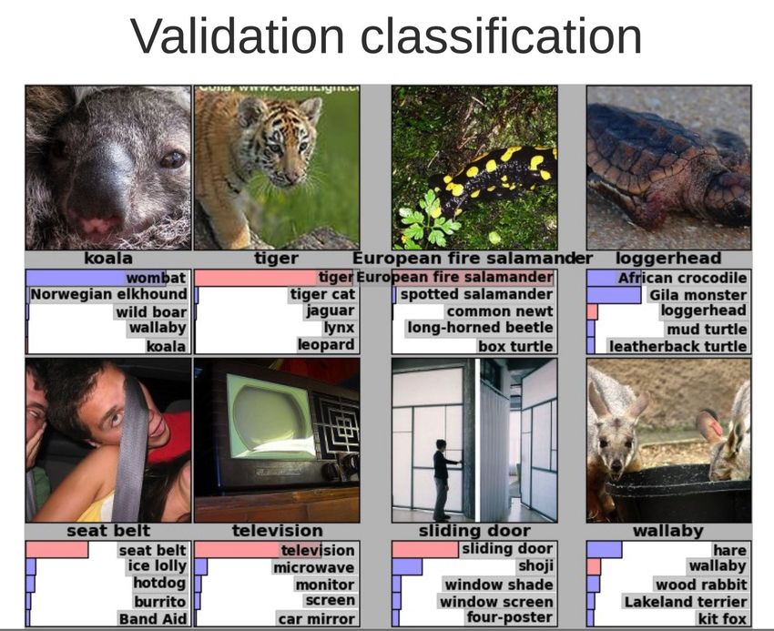
THE FIRST HIGH PERFORMANCE CNN: ALEXNET
•    NN based on the architecture of Krizhevsky et Al. winner of Imagnet 2012 Contest
•    developed under Caffe framework (Berkeley Vision Deep Learning framework: http://caffe.berkeleyvision.org)
•    instructions to install it on mac os x: https://vimeo.com/101582001

same top-down approach as LeNet with successive filters designed to capture more and more subtle features

+        improvements:
    1. better back-propagation via ReLU
    2. dropout based regularisation
    3. batch normalisation
    4. data augmentation: images presented
        to the NN during training with random
       translation, rotation, crop
    5. deeper architecture: more convolutional
       layers (7), i.e. more finer features
       captured

                                                                                      AlexNET
                                                                                                                  42
• feature initialised with white gaussian
noise
• fully supervised training
• training on GPU NVIDIA for ~1 week
• 650K neurons
• 60M parameters
• 630M connections
4344
45
46
You can also read