Mitosis Detection in Breast Cancer Histology Images with Deep Neural Networks
←
→
Page content transcription
If your browser does not render page correctly, please read the page content below
Mitosis Detection in Breast Cancer Histology Images
                with Deep Neural Networks

    Dan C. Cireşan, Alessandro Giusti, Luca M. Gambardella, Jürgen Schmidhuber

    IDSIA, Dalle Molle Institute for Artificial Intelligence, USI-SUPSI, Lugano, Switzerland
                  {dan,alessandrog,luca,juergen}@idsia.ch

        Abstract. We use deep max-pooling convolutional neural networks to detect mi-
        tosis in breast histology images. The networks are trained to classify each pixel in
        the images, using as context a patch centered on the pixel. Simple postprocessing
        is then applied to the network output. Our approach won the ICPR 2012 mitosis
        detection competition, outperforming other contestants by a significant margin.

1    Introduction
The number of mitotic figures visible in histology sections is an important indicator
for cancer screening and assessment. Normally, the count is performed manually by
histologists, but automating the process could reduce its time and costs (thus making it
more accessible), minimize errors, and improve the comparability of results obtained in
different labs.
    Mitosis detection is very hard. In fact, mitosis is a complex process during which
a cell nucleus undergoes various transformations. In addition, different image areas are
characterized by different tissue types, which exhibit highly variable appearance. A
large amount of different structures can be observed in histology images stained with
Hematosin & Eosin, and in particular many dark-blue spots, most of which correspond
to cell nuclei. Only a subset of them is in a mitotic phase and must be detected. In most
stages a mitotic nucleus looks very much like a non-mitotic one, or like other dark-blue
spots, to the point that a human observer without extensive training cannot differentiate
them (Figure 1). As an additional complication, in later stages of the mitosis process a
nucleus may appear to split in two dark-blue spots, to be counted as one single mitosis.
    Our approach is conceptually very simple. We use a supervised Deep Neural Net-
work (DNN) as a powerful pixel classifier. The DNN is a max-pooling (MP) convo-
lutional neural network (CNN). It directly operates on raw RGB data sampled from a
square patch of the source image, centered on the pixel itself. The DNN is trained to
differentiate patches with a mitotic nucleus close to the center from all other windows.
Mitosis in unseen images are detected by applying the classifier on a sliding window,
and postprocessing its outputs with simple techniques. Because the DNN operates on
raw pixel values, no human input is needed : on the contrary, the DNN automatically
learns a set of visual features from the training data.
    Our main contribution is a new, important, practical application of DNN, which
recently produced outstanding results in image classification, segmentation and detec-
tion. Our approach is tested on a publicly available dataset. It significantly outperforms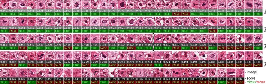
2

all competing techniques, with manageable computational effort: processing a 4MPixel
image requires few minutes on a standard laptop. Supplementary material for this paper
is available at http://bit.ly/18681Km.

Related Work Different flavors of CNN have been used for decades to classify objects.
Introduced in 1980 [6] and gradually improved over the next two decades [11,1,17],
they unfold their full potential when combined with MP and made both deep and wide
[3,4]. They excel on data sets ranging from handwritten characters [3] to complex clut-
tered images (NORB) [4], faces, and natural color images. DNN-based pattern recog-
nition is not limited to object classification, but can be used for detection as well. Re-
cently, DNN were used to segment images of neural tissue in Electron Microscopy [2]
and natural scenes [5].
     Many detection problems in biomedical images are solved by means of pixel clas-
sifiers, and are characterized by the relatively obvious appearance of the objects to be
detected. Difficulties may arise due to clumping/touching objects which may be hard to
separate and count [13]. Mitosis detection is different. While mitosis are normally rare
and well-separated, they are very hard to differentiate from non-mitotic nuclei.

2   Methods
Given an input RGB image I, the problem is to find a set D = {d1 , d2 , . . . , dN } of
detections, each reporting the centroid coordinates for a single mitosis. The problem is
solved by training a detector on training images with given ground truth information
about the centroid of each visible mitosis. Each pixel is assigned one of two possible
classes, mitosis or non-mitosis, the former to pixels at (or close to) mitosis centroids,
the latter to all other pixels. Our detector is a DNN-based pixel classifier. For any given
pixel p, the DNN predicts its class using raw RGB values in a square image window
centered on p (Figure 1). Windows of class mitosis contain a visible mitosis around the
window’s center. Others contain off-center or no mitosis.

Deep Neural Netwok architecture A DNN [4] is a feed-forward net made of succes-
sive pairs of convolutional and max-pooling layers, followed by several fully connected
layers. Raw pixel intensities of the input image are passed through this general, hier-
archical feature extractor. The feature vector it produces is classified by the fully con-
nected layers. All weights are optimized through minimization of the misclassification
error over the training set.
    Each convolutional layer performs a 2D convolution of its input maps with a rect-
angular filter. The filter is applied in every possible position of the input map. If the
previous layer contains more than one map, the activations of the corresponding convo-
lutions are summed up, then passed through a nonlinear activation function.
    One of the architectural differences between our DNN and previous CNN [11] are
max-pooling (MP) layers [14,16] instead of sub-sampling layers. Their outputs are
given by the maximum activations over non-overlapping square regions. MP layers are
fixed, non-trainable layers selecting the winning features. Typical DNN also are much
wider than previous CNN, with many more connections, weights and non-linearities.
3
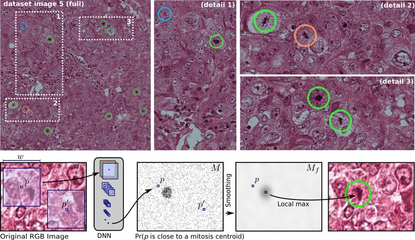
Fig. 1. Top left: one image (4 MPixels) corresponding to one of the 50 high power fields repre-
sented in the dataset. Our detected mitosis are circled green (true positives) and red (false posi-
tives); cyan denotes mitosis not detected by our approach. Top right: details of three areas (full-
size results on the whole dataset in supplementary material). Note the challenging appearance of
mitotic nuclei and other very similar non-mitotic structures. Bottom: overview of our detection
approach.
After several pairs of convolutional and MP layers, one fully connected layer fur-
ther mixes the outputs into a feature vector. The output layer is a simple fully connected
layer with one neuron per class (two for this problem), activated by a softmax function,
thus ensuring that each neuron’s output activation can be interpreted as the probability
of a particular input belonging to that class.
Training a detector Using ground truth data, we label each pixel of each training
image as either mitosis (when closer than d pixels to the centroid of a mitosis) or non-
mitosis (elsewhere). Then, we build a training set in which each instance maps a square
window of RGB values sampled from the original image to the class of the central
pixel. If a window lies partly outside of the image boundary, the missing pixels are
synthesized by mirroring.
The mitosis detection problem is rotationally invariant. Therefore, additional train-
ing instances are generated by transforming windows within the training set by applying
arbitrary rotations and/or mirroring. This is especially important considering that there
are extremely few mitosis examples in the training set.
Processing a testing image To process an unseen image I, we apply the DNN to
all windows whose central pixel is within the image boundaries. Pixels outside of the
image boundaries are again synthesized by mirroring. This yields a probability map4
M , in which each pixel is assigned a probability of being close to the centroid of a
mitosis. Ideally, we expect M to be zero everywhere except within d-pixel-radius disks
centered on each mitosis. In practice, M is extremely noisy. Therefore, M is convolved
with a d-pixel-radius disk kernel, which yields a smoothed probability map Mf ; the
local maxima of Mf are expected to lie at the disk centers in M , i.e., at the centroids of
each mitosis.
To obtain a set of detections DI for image I, we first initialize DI ← ∅, then iterate
the following two steps until no pixel in Mf exceeds a given threshold t.
– Let pm be the pixel with the largest value in Mf ; DI = DI ∪ (pm , Mf (pm )).
– Mf (p) ← 0 for each p : |p − pm | < 2d (non-maxima suppression).
This yields a (possibly empty) set DI (depending on threshold t) containing the detected
centroids of all mitosis in image I, as well as their respective score.
Exploiting multiple nets and rotational invariance Because the DNN classifier is
very flexible and has many degrees of freedom, it is expected to exhibit large variance
and low bias [7]. In fact, in related work [2] it was observed that large nets with different
architectures, even when trained on the same dataset, tend to yield significantly different
outputs, especially for challenging image parts. We reduce such variance by averaging
the outputs of multiple classifiers with different architectures. Moreover, we exploit
rotational invariance by separately processing rotated and mirrored versions of each
input image, and averaging their results.
3 Materials, Experiments and Results
Dataset and Performance Measures We evaluate our method on the public MITOS
dataset including 50 images corresponding to 50 high-power fields in 5 different biopsy
slides stained with Hematosin & Eosin. A total of about 300 mitosis are visible in
MITOS. Each field represents a 512×512µm2 area, and is acquired using three different
setups: two slide scanners and a multispectral microscope. Here we consider images
acquired by the Aperio XT scanner, the most widespread and accessible solution among
the three. It has a resolution of 0.2456µm per pixel, resulting in a 2084 × 2084 RGB
image for each field. Expert pathologists manually annotated all visible mitosis.
We partition the 50 images into three subsets: T1 (26 images), T2 (9 images), and
T3 (15 images). T3 coincides with the evaluation images for the 2012 ICPR Mitosis
Detection Contest. Its ground truth was withheld from contestants until the end of the
contest. T3 is exclusively used for computing our performance measures once, to ensure
a fair comparison with other algorithms.
Given a set of detections for dataset T3, according to the contest criteria, we count
the number NTP of True Positives (i.e. detections whose coordinates are closer than
5µm(20 px) from the ground truth centroid), False Positives (NFP ) and False Negatives
(NFN ). We compute the following performance measures: recall (R = NTP /(NTP +
NFN )), precision (P = NTP /(NTP + NFP )) and F1 score (F1 = 2P R/(P + R)).
We randomly split the remaining 35 images, for which ground truth was available,
in two disjoint sets T1 (training) and T2 (validation). Detectors trained on the former
are evaluated on the latter for determining the threshold yielding the largest F-score.5
Building the detector For images in T1 and T2, the mitosis class is assigned to all win-
dows whose center pixel is closer than d = 10 pixels to the centroid of a ground-truth
mitosis; all remaining windows are given the non-mitosis class. This results in a total
of roughly 66000 mitosis pixels and 151 million non-mitosis pixels. Note that, among
all non-mitosis pixels, only a tiny fraction (i.e. those close to non-mitotic nuclei and
similarly looking structures) represent interesting instances. In contrast, the largest part
of the image area is covered by background pixels far from any nucleus, whose class
(non-mitosis) is quite trivial to determine. If training instances for class non-mitosis
were uniformly sampled from images, most of the training effort would be wasted.
Other approaches [18,8,12,20] address this issue by first detecting all nuclei, then
classifying each nucleus separately as mitotic or non-mitotic. We follow a different,
simpler approach, which does not need any additional ground-truth information and
relies on a single trained detector. In particular, we build our training set so that the rel-
atively rare challenging non-mitosis instances are well represented, whereas instances
obviously belonging to class non-mitosis (which prevail in the input images) appear
only rarely. This approach, loosely inspired by boosting techniques, allows us to spend
most of the training time in learning important differences among mitotic and non-
mitotic nuclei. We adopt a general approach to building such a training set, without
relying on problem-specific heuristics.
– We build a small training set Sd, which includes all 66000 mitosis instances and the
same number of non-mitosis instances, uniformly sampled from the 151 million
non-mitosis pixels.
– We use Sd to briefly train a simple DNN classifier Cd. Because Cd is trained on a
limited training set in which challenging non-mitosis instances are severely under-
represented, it tends to misclassify most non-mitotic nuclei as class mitosis.
– We apply Cd to all images in T1 and T2. Let D(p) denote the mitosis probability
that Cd assigns to pixel p. D(p) will be large for challenging non-mitosis pixels.
– We build the actual training set, composed by 1 million instances, which includes
all mitosis pixels (6.6% of the training instances). The remaining 95.4% is sampled
from non-mitosis pixels by assigning to each pixel p a weight D(p).
The resulting optimized training set is used for learning two nets DNN1 and DNN2
(architectures outlined in Table 1). Because the problem is rotationally invariant, during
each training epoch each patch is subject to a random rotation around its center and a
50% chance of mirroring, in order to artificially augment the training set.
Each unseen image I is processed 16 times: each of the two nets is applied to each
of 8 variations of the input image, namely: rotations by k · 90◦ , k = 0, 1, 2, 3, with
and without mirroring. For each variation, the resulting map is subject to the inverse
transformation, to match the input image. The resulting 16 maps are averaged, yielding
M , from which a set of detections DI is determined as described in Section 2.
The whole procedure is first performed by training the nets on data from T1 and
detecting mitosis in T2 images. The threshold yielding the largest F1 score (t0 = 0.35)
is then determined. The final detector is obtained by training the two nets on data from
T1 and T2, and evaluated on T3.
Training each network requires one day of computation with an optimized GPU
implementation. Less than 30 epochs are needed to reach a minimum on validation6
Table 1. 13-layer architecture for network DNN1 (left) and 11-layer architecture for network
DNN2 (right). Layer type: I - input, C - convolutional, MP - max-pooling, FC - fully-connected.
Layer Type Maps Filter Weights Connections
and neurons size Layer Type Maps Filter Weights Connections
and neurons size
0 I 3M x 101x101N — — —
1 C 16M x 100x100N 2x2 208 2080000 0 I 3M x 101x101N — — —
2 MP 16M x 50x50N 2x2 — — 1 C 16M x 98x98N 4x4 784 7529536
3 C 16M x 48x48N 3x3 2320 5345280 2 MP 16M x 49x49N 2x2 — —
4 MP 16M x 24x24N 2x2 — — 3 C 16M x 46x46N 4x4 4112 8700992
5 C 16M x 22x22N 3x3 2320 1122880 4 MP 16M x 23x23N 2x2 — —
6 MP 16M x 11x11N 2x2 — — 5 C 16M x 20x20N 4x4 4112 1644800
7 C 16M x 10x10N 2x2 1040 104000 6 MP 16M x 10x10N 2x2 — —
8 MP 16M x 5x5N 2x2 — — 7 C 16M x 8x8N 3x3 2320 148480
9 C 16M x 4x4N 2x2 1040 16640 8 MP 16M x 4x4N 2x2 — —
10 MP 16M x 2x2N 2x2 — — 9 FC 100N 1x1 25700 25700
11 FC 100N 1x1 6500 6500 10 FC 2N 1x1 202 202
12 FC 2N 1x1 202 202
data. For detecting mitosis in a single image, our MATLAB implementation required
31 seconds to apply each network on each input variation, which amounts to a total time
of roughly 8 minutes per image. Significantly faster results can obtained by averaging
fewer variations with minimal performance loss (see Table 2).
Performance and Comparison Performance results on the T3 dataset are reported in
Table 2. Our approach yields an F-score of 0.782, significantly higher than the F-score
obtained by the closest competitor (0.718). The same data is plotted in the Precision-
Recall plane in Figure 3.
The choice of the detection threshold t affects the resulting F-score: Figure 3 (right)
shows that the parameter is not particularly critical, since even significant deviations
from t0 result in limited performance loss.
Table 2. Performance results for our approach (DNN) compared with competing approaches [15].
We also report the performance of faster but less accurate versions of our approach, namely:
DNNf12, which averages the results of nets DNN1 and DNN2 without computing input variations
(1 minute per image), and DNNf1, which is computed only from the result of DNN1 (31s per
image).
method precision recall F1 score method precision recall F1 score
DNN 0.88 0.70 0.782 NUS 0.63 0.40 0.490
DNNf12 0.85 0.68 0.758 ISIK [19] 0.28 0.68 0.397
DNNf1 0.78 0.72 0.751 ETH-HEILDERBERG [18] 0.14 0.80 0.374
IPAL [9] 0.69 0.74 0.718 OKAN-IRISA-LIAMA 0.78 0.22 0.343
SUTECH 0.70 0.72 0.709 IITG 0.17 0.46 0.255
NEC [12] 0.74 0.59 0.659 DREXEL 0.14 0.21 0.172
UTRECHT [20] 0.51 0.68 0.583 BII 0.10 0.32 0.156
WARWICK [10] 0.46 0.57 0.513 QATAR 0.00 0.94 0.0057
Fig. 2. All 143 detections (29 per row) on T3 with scores larger than 0.1, sorted by descend-
ing score. For each, we report the corresponding image patch, score, and whether it is a mitosis
(TRUE, bright green background) or a non-mitosis (FALSE, dark red background). Vertical dot-
ted line for score 0.35 reports the detection threshold t0 determined on T2.
Fig. 3. Left: Performance of our approach compared to others in the PR plane. Right: sensitivity
to the choice of threshold.
4 Conclusion and Future Works
We presented an approach for mitosis detection that outperformed all competitors on
the first public annotated dataset of breast cancer histology images.
Future work will aim at validating our approach on larger datasets, and comparing
its performance to the one of expert histologists, with the ultimate goal of gradually
bringing automated mitosis detection into clinical practice.
Acknowledgments
This work was partially supported by the Supervised Deep / Recurrent Nets SNF grant,
Project Code 140399.8
References
1. Behnke, S.: Hierarchical Neural Networks for Image Interpretation, Lecture Notes in Com-
puter Science, vol. 2766. Springer (2003) 2
2. Ciresan, D.C., Giusti, A., Gambardella, L.M., Schmidhuber, J.: Deep Neural Networks Seg-
ment Neuronal Membranes in Electron Microscopy Images. In: Neural Information Process-
ing Systems. pp. 2852–2860 (2012) 2, 4
3. Ciresan, D.C., Meier, U., Masci, J., Gambardella, L.M., Schmidhuber, J.: Flexible, High
Performance Convolutional Neural Networks for Image Classification. In: International Joint
Conference on Artificial Intelligence. pp. 1237–1242 (2011) 2
4. Ciresan, D.C., Meier, U., Schmidhuber, J.: Multi-column Deep Neural Networks for Image
Classification. In: Computer Vision and Pattern Recognition. pp. 3642–3649 (2012) 2
5. Farabet, C., Couprie, C., Najman, L., LeCun, Y.: Learning Hierarchical Features for Scene
Labeling. IEEE Transactions on Pattern Analysis and Machine Intelligence (2013), in press
2
6. Fukushima, K.: Neocognitron: A self-organizing neural network for a mechanism of pattern
recognition unaffected by shift in position. Biological Cybernetics 36(4), 193–202 (1980) 2
7. Geman, S., Bienenstock, E., Doursat, R.: Neural networks and the bias/variance dilemma.
Neural computation 4(1), 1–58 (1992) 4
8. Huang, C., Hwee, K.: Automated Mitosis Detection Based on Exclusive Independent Com-
ponent Analysis. In: Proc. ICPR 2012 (2012) 5
9. Irshad, H.: Automated mitosis detection in histopathology using morphological and multi-
channel statistics features. Journal of Pathology Informatics 4(1) (2013) 6
10. Khan, A., ElDaly, H., Rajpoot, N.: A gamma-gaussian mixture model for detection of mitotic
cells in breast cancer histopathology images. Journal of Pathology Informatics 4(1) (2013) 6
11. LeCun, Y., Bottou, L., Bengio, Y., Haffner, P.: Gradient-Based Learning Applied to Docu-
ment Recognition. Proceedings of the IEEE 86(11), 2278–2324 (November 1998) 2
12. Malon, C., Cosatto, E.: Classification of mitotic figures with convolutional neural networks
and seeded blob features. Journal of Pathology Informatics 4(1) (2013) 5, 6
13. Pan, J., Kanade, T., Chen, M.: Heterogeneous conditional random field: Realizing joint de-
tection and segmentation of cell regions in microscopic images. In: Computer Vision and
Pattern Recognition, 2010 IEEE Conference on. pp. 2940–2947. IEEE (2010) 2
14. Riesenhuber, M., Poggio, T.: Hierarchical models of object recognition in cortex. Nat. Neu-
rosci. 2(11), 1019–1025 (1999) 2
15. Roux, L., Racoceanu, D., Lomnie, N., Kulikova, M., Irshad, H., Klossa, J., Capron, F., Gen-
estie, C., Naour, G.L., Gurcan, M.N.: Mitosis detection in breast cancer histological images
An ICPR 2012 contest. Journal of Pathology Informatics 4(1) (2013) 6
16. Scherer, D., Müller, A., Behnke, S.: Evaluation of Pooling Operations in Convolutional Ar-
chitectures for Object Recognition. In: International Conference on Artificial Neural Net-
works (2010) 2
17. Simard, P.Y., Steinkraus, D., Platt, J.C.: Best practices for convolutional neural networks ap-
plied to visual document analysis. In: Seventh International Conference on Document Anal-
ysis and Recognition. pp. 958–963 (2003) 2
18. Sommer, C., Fiaschi, L., Heidelberg, H., Hamprecht, F., Gerlich, D.: Learning-based mitotic
cell detection in histopathological images. In: Proc. ICPR 2012 (2012) 5, 6
19. Tek, F.: Mitosis detection using generic features and an ensemble of cascade adaboosts.
Journal of Pathology Informatics 4(1) (2013) 6
20. Veta, M., van Diestb, P., Pluim, J.: Detecting mitotic figures in breast cancer histopathology
images. In: Proc. of SPIE Medical Imaging (2013) 5, 6You can also read