Unsupervised Learning in Reservoir Computing: Modeling Hippocampal Place Cells for Small Mobile Robots
←
→
Page content transcription
If your browser does not render page correctly, please read the page content below
Unsupervised Learning in Reservoir Computing:
 Modeling Hippocampal Place Cells for Small
               Mobile Robots

                    Eric A. Antonelo⋆ and Benjamin Schrauwen

         Electronics and Information Systems Department, Ghent University,
                   Sint Pietersnieuwstraat 41, 9000 Ghent, Belgium
               {eric.antonelo,benjamin.schrauwen}@elis.ugent.be
                            http://reslab.elis.ugent.be

        Abstract. Biological systems (e.g., rats) have efficient and robust local-
        ization abilities provided by the so called, place cells, which are found in
        the hippocampus of rodents and primates (these cells encode locations
        of the animal’s environment). This work seeks to model these place cells
        by employing three (biologically plausible) techniques: Reservoir Com-
        puting (RC), Slow Feature Analysis (SFA), and Independent Component
        Analysis (ICA). The proposed architecture is composed of three layers,
        where the bottom layer is a dynamic reservoir of recurrent nodes with
        fixed weights. The upper layers (SFA and ICA) provides a self-organized
        formation of place cells, learned in an unsupervised way. Experiments
        show that a simulated mobile robot with 17 noisy short-range distance
        sensors is able to self-localize in its environment with the proposed ar-
        chitecture, forming a spatial representation which is dependent on the
        robot direction.

        Key words: reservoir computing, slow feature analysis, place cells

1     Introduction
Animals or robots should be able to efficiently self-localize in their environments
for learning and accomplishing cognitive intelligent behaviors. They must be able
to seek targets (energy resources) and accomplish important tasks in a efficient
way. In this context, the ability to self-localize is clearly needed.
    Standard robot localization systems are designed mostly by probabilistic
methods which can perform SLAM (Simultaneous Localization And Mapping)
under suitable assumptions [1] and are usually built for robots having high-
resolution expensive laser scanners. Biologically inspired systems for robot lo-
calization can be considered a competitive alternative that works also for small
mobile robots. Robustness, learning and low computation time are some charac-
teristics of these biological inspired systems. Most systems are based on visual
input from camera [2–4] and models hippocampal place cells from rats [2–5].
⋆
    This work was partially supported by FWO Flanders project G.0317.05.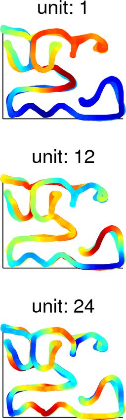
2       Unsupervised Learning in Reservoir Computing: Modeling Place Cells

These place cells are the main components of the spatial navigation system in
rodents. Each place cell codes for a particular location of the rat’s environment,
presenting a peak response in the proximities of that location (the place field
of that cell). Other components of the brain’s spatial representation system in-
cludes head-direction cells, which encode the orientation of the animal in its
environment, and grid cells, which are non-localized representations of space
(having a grid-like structure of activations in space) [6]. Grid cells are found in
the entorhinal cortex of rats and probably have an important role in the forma-
tion of place cells in the hippocampus [6]. Two classes of stimuli are available to
place and grid cells: idiothetic and allothetic. Idiothetic input is originated from
the physical body, such as proprioceptive sensors, which can be used for dead
reckoning (path integration). Allothetic information is obtained from the exter-
nal environment via sensors like distance sensors and camera. Dead reckoning
can usually be corrected using allothetic information. The current work models
place cells and to some extent, grid cells, endowing a simulated mobile robot with
the capacity to self-localize in its environment through an unsupervised learn-
ing process. Reservoir Computing (RC) [7, 8], Slow Feature Analysis (SFA) [9],
and Independent Component Analysis (ICA) [10] are three (biologically plau-
sible) techniques used in this work for modeling place cells. RC is a recently
introduced paradigm in Recurrent Neural Networks (RNN) where the recurrent
connections are not trained at all. Only output units are trained (usually in a
supervised way) while the reservoir (the RNN itself) is a randomly generated
dynamic system with fixed weights [8]. RC has biological foundations as it is
shown, for example, that Liquid State Machines (a type of RC) are based on the
micro-column structure in the cortex [11]. Furthermore, works such as in [12]
establish a strong association between real brains and reservoirs. SFA is another
recently proposed method to extract invariant or slowing varying features from
input data [9]. Similarly to [3], we use SFA to model grid cells. While they use
several SFA layers and high-dimensional input from a camera, we use only few
noisy distance sensors and a RC-SFA based architecture.
    This work proposes a general architecture based on reservoir computing and
slow feature analysis (RC-SFA). While SFA provides an unsupervised learning
mechanism for reservoirs, the latter provides short-term memory to SFA-based
systems. This powerful combination can also be used in more general applica-
tions (such as speech recognition and robot behavior modeling). The proposed
architecture is used here for autonomous map learning by modeling hippocampal
place cells. A mobile robot with 17 short-range distance sensors is sufficient for
generating a rather accurate spatial representation of maze-like environments
without using proprioceptive information (odometry). The robot, in this way,
autonomously learns to self-localize in its environment.

2     Methods
2.1   Reservoir Computing
The first layer of the RC-SFA architecture consists of a randomly created recur-
rent neural network, that is, the reservoir. This network is composed of sigmoidal
Unsupervised Learning in Reservoir Computing: Modeling Place Cells 3
neurons and is modeled by the following state update equation [8]:
x(t + 1) = f ((1 − α)x(t) + α(Win u(t) + Wres x(t))), (1)
where: u(t) denotes the input at time t; x(t) represents the reservoir state; α is
the leak rate [13]; and f () = tanh() is the hyperbolic tangent activation function
(the most common type of activation function used for reservoirs). The con-
nections between the nodes of the network are represented by weight matrices:
Win is the connection matrix from input to reservoir and Wres represents the
recurrent connections between internal nodes. The initial state of the dynamical
system is x(0) = 0. A standard reservoir equation (without the leak rate) is
found when α = 1.
The matrices Win and Wres are fixed and randomly created at the beginning.
Each element of the connection matrix Wres is drawn from a normal distribution
with mean 0 and variance 1. The randomly created Wres matrix is rescaled such
that the system is stable and the reservoir has the echo state property (i.e., it
has a fading memory [8]). This can be accomplished by rescaling the matrix so
that the spectral radius |λmax | (the largest absolute eigenvalue) of the linearized
system is smaller than one [8]. Standard settings of |λmax | lie in a range between
0.7 and 0.98 [8]. In this work we scale all reservoirs (Wres ) to a spectral radius
of |λmax | = 0.9 which is an arbitrarily chosen value (shown to produce good
results). The initialization of Win is given in Section 3.1.
The leak rate α should be in the interval (0, 1] and can be used to tune
the dynamics of the reservoir [13]. In this way, lower leak rates slow down the
reservoir, increasing its memory but decreasing its capacity for agile processing
of the input signal. Higher leak rates yield fast processing of the input but low
memory to hold past stimuli. Similar results can be achieved when resampling
the input signal for matching the timescale of the reservoir. For instance, it might
be necessary to downsample an input signal if it varies too slowly. In this work,
dt represents the downsampling rate of the original input signal.
In this paper, the RC-SFA architecture is composed of a hierarchical network
of nodes where the lower layer is the reservoir and the upper layers are composed
of SFA and ICA units, respectively (Fig. 1). This hierarchical network learns in
a unsupervised way (except for the reservoir whose weights (Win and Wres )
are kept fixed). The function of the reservoir is to map the inputs to a high-
dimensional dynamic space. Because of its recurrent connections, the reservoir
states contain echoes of the past inputs, providing a short-term memory to our
model. The SFA layer receives signals from the input nodes u(t) and from the
reservoir nodes x(t). This layer generates invariant or slowly varying signals [9]
which are instantaneous functions of input from previous layers (see Section 2.2).
The upper-most layer is composed of ICA units which generate a sparse and local
representation of the slowing varying SFA features. The following sections focus
on these upper layers. Next, consider nu as the number of inputs; nres as the
number of neurons in the reservoir; nsfa as the number of SFA units; and nica as
the number of ICA units.4 Unsupervised Learning in Reservoir Computing: Modeling Place Cells
2.2 Slow Feature Analysis
Slow Feature Analysis (SFA) is a recently introduced algorithm that finds func-
tions which are independent and slowly varying representations of the input [9].
SFA has also been shown to reproduce qualitative and quantitative properties
of complex cells found in the primary visual cortex (V1) [14] and grid-cells from
the entorhinal cortex of rats [3].
The learning task can be defined as follows. Given a high-dimensional input
signal x(t), find a set of scalar functions gi (x(t)) so that the SFA output yi =
gi (x(t)) varies as slowly as possible and still carries significant information. In
mathematical terms [9], find output signals yi = gi (x(t)) such that:
∆(yi ) := hẏi2 it is minimal (2)
under the constraints
hyi it = 0 (zero mean) (3)
hyi2 it = 1 (unit variance) (4)
∀j < i, hyi yj it = 0 (decorrelation and order) (5)
where h.it and ẏ denote temporal averaging and the derivative of y, respectively.
Learning: Before applying the algorithm, the input signal x(t) is normalized
to have zero mean and unit variance. In this work, we only consider the linear case
gi (x) = wT x, because the reservoir is already non-linear. The SFA algorithm is
as follows:
Solve the generalized eigenvalue problem:
AW = BWΛ, (6)
T T
where A := hẋẋ it and B := hxx it .
The eigenvectors w1 , w2 , ..., wnsf a corresponding to the ordered generalized eigen-
values λ1 ≤ λ2 ≤ ... ≤ λnsf a solve the learning task, satisfying (3-5) and min-
imizing (2) (see [9] for more details). This algorithm is guaranteed to find the
global optimum.
Architecture: The SFA layer in our architecture (Fig. 1) is denoted by ysfa (t):
ysfa (t) = Wsfa xsfa (t), (7)
where: xsfa (t) is the input vector at time t consisting of a concatenation of
input u(t) and reservoir states x(t). Note that the states x(t) are generated
by stimulating the reservoir with the input signal u(t) for t = 1, 2, ...ns by
using (1), where ns is the number of samples. The connection matrix Wsfa is a
nsfa × (nu + nres ) matrix corresponding to the eigenvectors found by solving (6).
In this work, the output signal ysfa (t) generates non-localized representations of
the environment, similarly to grid cells of the entorhinal cortex of rats [6].
2.3 Independent Component Analysis
Independent Component Analysis (ICA) is a method used for sparse coding
of input data as well as for blind source separation [10]. The ICA model as-
sumes that a linear mixture of signals x1 , x2 ...xn can be used for finding theUnsupervised Learning in Reservoir Computing: Modeling Place Cells 5
n independent components or latent variables s1 , s2 ...sn . The observed values
x(t) = [x1 (t), x2 (t)...xn (t)] can be written as:
x(t) = As(t) (8)
where A is the mixing matrix; and s(t) = [s1 (t), s2 (t)...sn (t)] is the vector of
independent components (both A and s(t) are assumed to be unknown). The
vector s(t) can be generated after estimating matrix A:
s(t) = Wx(t) (9)
where W is the inverse matrix of A. The basic assumption for ICA is that
the components si are statistically independent. It is also assumed that the
independent components have nongaussian distributions [10].
Learning: In this work the matrix W is found with the FastICA algorithm
[10]. Before using ICA, the observed vector x(t) is preprocessed by centering
(zero-mean) and whitening (decorrelation and unit variance) [10]. FastICA uses
a fixed-point iteration scheme for finding the maximum of the nongaussianity of
wx(t) (where w is a weight vector of one neuron). The basic form of the FastICA
algorithm (for one unit) is described next:
1. Initialize w randomly
2. Let w+ = E{xg(wT x)} − E{g ′ (wT x)w}
3. Let w = w+ /kw+ k
4. Do steps 2 and 3 until convergence,
where g is the derivative of a nonquadratic function G (in this work, G(u) = u3 )
(see [10] for a detailed description).
Architecture: The equation for the ICA layer is (by redefining variables):
yica (t) = Wica ysfa (t), (10)
where: ysfa (t) is the input vector at time t (the observed values); Wsfa is the
mixing matrix (nica × nsfa ); and yica (t) is the output of the ICA layer (the inde-
pendent components), which, in this work, learns to generate localized outputs
which model hippocampal place cells of rats [6].
2.4 Robot Model
The robot model used in this work (Fig. 1) is part of the 2D SINAR simulator
[15] and is described next. The robot interacts with the environment by distance
and color sensors; and by one actuator which controls the movement direction
(turning). Seventeen (17) sensor positions are distributed uniformly over the
front of the robot (from -90◦ to +90◦ ). Each position holds two virtual sensors
(for distance and color perception) [15]. The distance sensors are limited in
range (i.e., they saturate for distances greater than 300 distance units (d.u.))
and are noisy (they exhibit Gaussian noise on their readings, generated from
N (0, 0.01)). A value of 0 means near some object and a value of 1 means far
or nothing detected. At each iteration the robot is able to execute a direction
adjustment to the left or to the right in the range [0, 15] degrees and the speed
is constant (0.28 distance units (d.u.)/s). The SINAR controller (based on [15])
is an intelligent navigation system made of hierarchical neural networks which6 Unsupervised Learning in Reservoir Computing: Modeling Place Cells
(b)
(a) (c)
Fig. 1. (a) RC-SFA architecture. (b) Robot model. (c) Environment E1. The environ-
ment is tagged with 64 labels displayed by small triangles.
learn by interaction with the environment. After learning, the robot is able to
efficiently navigate and explore environments, during which the signal u(t) is
built by recording the 17 distance sensors of the robot.
3 Experiments
3.1 Introduction
In the following, we describe the architecture (Fig. 1) and the initialization of
parameters for the experiments. The first layer of the architecture corresponds
to a dynamic reservoir of 400 neurons, which provides short-term memory to
our model. The second layer consists of 70 SFA units, which extracts the slow
features from the reservoir states and distance sensors. The output of the SFA
layer models the grid cells found in the entorhinal cortex of primates [6], similarly
to the simulated rat’s grid cells formed from visual input in [3]. The last layer
is composed of 70 ICA units, which model place cells usually found in the CA
areas of the hippocampus [6]. Grid cells are non-localized in the sense that they
fire for more than a single location while place cells encode a specific position of
the animal’s environment.
As the robot has a very low speed, the input signal (17 distance sensors)
is downsampled by a factor of dt = 50 (using the matlab function resample).
Additionally, the leak rate in the reservoir is set to α = 0.6. These settings,
optimized for the supervised scheme in [16], worked well for the current work
(optimization and performance analysis of these parameters is left as future
work). The matrix connecting the input to the reservoir (Win ) is initialized to
-0.2, 0.2 and 0 with probabilities 0.15, 0.15 and 0.7, respectively.
The experiments are conducted using environment E1 (Fig. 1). It is a big
maze with 64 predefined locations spread evenly around the environment (rep-
resented by small labeled triangles). First, for generating the input signal, theUnsupervised Learning in Reservoir Computing: Modeling Place Cells 7
simulated robot navigates in the environment for 350.000 timesteps while its dis-
tance sensor measurements are recorded (the robot takes approximately 13.000
timesteps to visit most of the locations). The controller basically makes the
robot explore the whole environment. After dowsampling the recorded input
signal u(t), the number of samples becomes ns = 7.000. Next, the downsampled
input signal is used to generate the reservoir states x(t), t = 1, 2, ..., ns using (1).
The learning of the RC-SFA architecture takes place in 2 steps and uses
5/6 of the input signal as the training dataset (1/6 for testing). First, the SFA
layer learns by solving (6) where the inputs are the reservoir states and distance
sensors (like in (7)). After Wsfa is found, the output of SFA units ysfa (t), t =
1, 2, ..., ns is generated using (7). The second step corresponds to the learning of
the upper ICA layer by applying the FastICA algorithm from Section 2.3 where
the inputs for this layer are the output of the SFA units. The output signals
ysfa (t) and yica (t) are upsampled to the original sampling rate of u(t).
3.2 Results
The RC-SFA architecture is trained sequentially from the middle SFA layer to
the top ICA layer. This section shows the results after training the layers with
the input signal u(t) and reservoir states x(t) generated with the previously
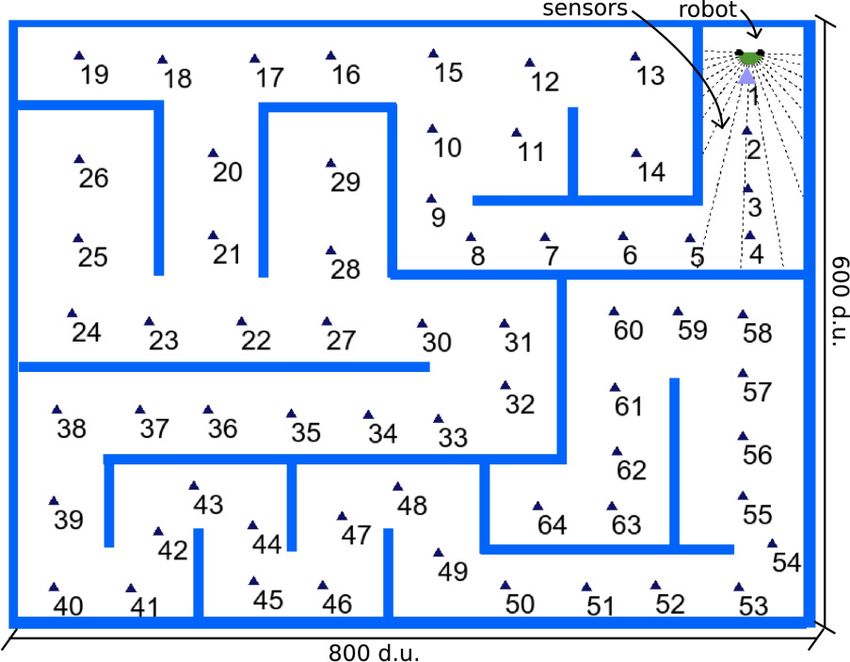
presented setup. Fig. 2(a) shows the output of 3 SFA units for a test input
signal. The left plots show the outputs over time whereas the right plots show the
response of the neurons as a function of the robot position in the environment.
In the left plot, the horizontal axis represents the time, the left vertical axis
denotes the real robot location (as given by the labeled triangles in Fig. 1),
and the right vertical axis denotes the SFA output of the neuron. The colored
dots represent the output of the SFA unit (where red denotes a peak response,
green an intermediate response, and blue a low response). The SFA output is
also shown as a black line in the same plot and as a colored trajectory in the
right plot. As SFA units are ordered by slowness, the first SFA unit has the
slowest response. It is high only for two areas of the environment: locations 10
to 17, and locations 27 to 35. Units 12 and 24 vary much faster, encoding several
locations of the environment. In the same figure, it is possible to observe that
SFA units learn a representation which is dependent on the robot heading. For
instance, unit 12 responds differently for trajectories which go towards location
64 and trajectories that start from this position. As slow feature analysis is a
method which is highly dependent on the input statistics, the movement patterns
generated by the robot controller decisively influence the learning of the SFA
units. In this context, most SFA units learn to be robot direction dependent in
the current experiment. However, if the robot would change its direction more
often (or faster compared to its speed), the SFA unit could learn to be direction
invariant (by learning the slow features, that is, the robot position).
The upper ICA layer builds on the SFA layer. During learning, ICA units seek
to maximize nongaussianity so that their responses become sparse and clustered
and also as independent as possible. This form of sparse coding lead to the
unsupervised formation of place cells. Fig. 2(b) shows a number of ICA units8 Unsupervised Learning in Reservoir Computing: Modeling Place Cells
which code for specific locations in the environment. These units were chosen
such that they code for adjacent locations as if the robot was navigating in
the environment. The peak response is represented by white dots while lower
responses are given gradually in darker colors. In order to view the localized
aspect of place cells more clearly, the output of ICA units are ordered such that
they have a spatial relationship. The reference locations (from 1 to 64), shown
in environment E1 (Fig. 1), are used to automatically order the ICA layer.
ICA units which do not respond strongly enough (that is, less than 4.5) in any
situation are set to the end of the vector. Fig. 3(a) shows the real occupancy grid
for the robot while it drives in environment E1 and the respective ICA activation
map showing the spatially-ordered ICA responses (where u(t) is a test signal not
used during learning). The peak responses are shown in black while white dots
represent lower responses. Eleven ICA units (from 59 to 70) did not fire strongly
enough and, so, did not code for any location. This activation map is very similar
to the real robot occupancy grid showing that the place cells efficiently mapped
most of the environment. Fig. 3(b) shows a magnification of the ICA activation
map for locations under 20. It is possible to note that for almost the whole time
period there is only a single ICA unit active (i.e., the ICA layer is detecting
locations most of the time). This figure also clearly shows that most ICA units
are dependent on the robot direction (as SFA units are). We have repeated
the experiments shown here with the same datasets more than 15 times (where
for each time a different random reservoir is created) with no visible changes
in the learned place cells. Furthermore, preliminary results show that the RC-
SFA architecture also works for other kinds of environment configurations and
environments with dynamic objects.
unit: 1
Real Location
2
SFA output
60
40 0
20
−2
unit: 12
Real Location
2
SFA output
60
40 0
20
−2
unit: 24
Real Location
2
SFA output
60
40 0
20
−2
0 1 2 3 4 5 6
Timesteps 4
x 10
(a) SFA output (b) ICA output
Fig. 2. Results for simulations in Environment E1. (a) Responses of SFA units 1, 12,
and 24. Left: the SFA output over time. For each location (in time) given by the labeled
triangles in Fig. 1, there is a colored dot where red denotes a peak response, green an
intermediate response, and blue a low response. The output is also plot as a black line.
Right: the same SFA output as a function of the robot position. (b) Response of ICA
units as a function of the robot position. White dots denote high activity while darker
dots represent lower responses. The results show the localized aspect of place cells or
ICA units (the peak response is characteristic of one specific location).Unsupervised Learning in Reservoir Computing: Modeling Place Cells 9
Occupancy grid
Real robot location
60 ICA Activation Map
20
40
ICA Units
15
20 10
5
10 20 30 40 50 49 50 51 52 53 54 55 56
Timesteps (x 103) 3
Timesteps (x 10 )
(a) (b)
Fig. 3. Emergence of place cells in environment E1. (a) The real robot occupancy grid
(left) and the respective spatially-ordered ICA activation map (black dots denote peak
responses and white represent lower responses). (b) Close view of the ICA activation
map where green denotes low response and blue high response.
unit: 1
2
Real Location
SFA output
60
40 0
20
−2
0 1 2 3 4 5 6
Timesteps 4
x 10
1
Fig. 4. Results for modified architecture without the reservoir layer in environment
E1: the slowest SFA unit output over time, as in Fig. 2.
The importance of the reservoir can become more evident as it provides a
short-term memory of previous inputs. In order to compare results, the proposed
architecture in Fig. 1 is modified so that the inputs connect directly to the SFA
layer and no reservoir is used at all. The following changes are also accomplished:
the downsampling rate is increased to dt = 200 for slowing down the input signal;
nsfa = 100 and nica = 100. The SFA algorithm for this experiment includes
a quadratic expansion process on the inputs [9], making the SFA effectively
a non-linear process. The slowest SFA unit is shown in Fig. 4. The response
pattern from this unit seems more noisy than the case when using the RC-SFA
architecture which shows a smooth signal (Fig. 2(a)). The ICA activation map
for this architecture (not shown) was very fuzzy and far from the one obtained
in Fig. 3 (also did not solve the perceptual aliasing problem once one ICA unit
coded for multiple similar but distinct locations). In this way, this modified setup
without the reservoir was not able to model place cells in the current experiment.
4 Conclusion and Future Work
This work proposes a new biologically inspired architecture (RC-SFA) based on
a mixture of recently developed techniques (Reservoir computing, Slow Feature
Analysis and Independent Component Analysis). The RC-SFA is a general ar-
chitecture which can be easily applied to wide range of applications (e.g., extract
slowly-varying components of an input signal such as: behaviors or movements
of a humanoid robot or phonemes and words from speech data). In this work, a
simulated mobile robot (with few proximity sensors) autonomously learns, using
our proposed RC-SFA architecture, a rather accurate spatial representation of
its environment and, in this way, to self-localize in it. We do not use propriocep-
tive information as a form of spatial memory, but rather the short-term memory10 Unsupervised Learning in Reservoir Computing: Modeling Place Cells
of the reservoir has shown to eliminate the perceptual aliasing from sensors, pro-
ducing a system which autonomously learns the relevant information from the
input stream. Further interesting directions for research include the validation
of the proposed architecture with a real robot (such as the e-puck robot) and ac-
complish further experiments such as kidnapping the robot and navigation in a
dynamic environment. Other important questions include: how distinct settings
of reservoir parameters influence the learning of the spatial representation; what
kind of environments can be used; and what range of noise and sensor failures
the model can cope with.
References
1. Thrun, S., Burgard, W., Fox, D.: Probabilistic Robotics. The MIT Press (2005)
2. Arleo, A., Smeraldi, F., Gerstner, W.: Cognitive navigation based on nonuniform
gabor space sampling, unsupervised growing networks, and reinforcement learning.
IEEE Transactions on Neural Networks 15(3) (May 2004) 639–652
3. Franzius, M., Sprekeler, H., Wiskott, L.: Slowness and sparseness lead to place,
head-direction, and spatial-view cells. PLoS Comput. Biol. 3(8) (2007) 1605–1622
4. Stroesslin, T., Sheynikhovich, D., Chavarriaga, R., Gerstner, W.: Robust self-
localisation and navigation based on hippocampal place cells. Neural Networks
18(9) (2005) 1125–1140
5. Chavarriaga, R., Strsslin, T., Sheynikhovich, D., Gerstner, W.: A computational
model of parallel navigation systems in rodents. Neuroinformatics 3 (2005) 223–241
6. Moser, E.I., Kropff, E., Moser, M.B.: Place cells, grid cells and the brains spatial
representation system. Annual Reviews of Neuroscience 31 (2008) 69–89
7. Schrauwen, B., Verstraeten, D., Van Campenhout, J.: An overview of reservoir
computing: theory, applications and implementations. In: Proc. of ESANN. (2007)
8. Jaeger, H.: The “echo state” approach to analysing and training recurrent neural
networks. Technical Report GMD Report 148, German National Research Center
for Information Technology (2001)
9. Wiskott, L., Sejnowski, T.J.: Slow feature analysis: Unsupervised learning of in-
variances. Neural Computation 14(4) (2002) 715–770
10. Hyvärinen, A., Oja, E.: Independent component analysis: algorithms and applica-
tions. Neural Networks 13 (2000) 411–430
11. Maass, W., Natschläger, T., Markram, H.: Real-time computing without stable
states: A new framework for neural computation based on perturbations. Neural
Computation 14(11) (2002) 2531–2560
12. Yamazaki, T., Tanaka, S.: The cerebellum as a liquid state machine. Neural
Networks 20 (2007) 290–297
13. Jaeger, H., Lukosevicius, M., Popovici, D.: Optimization and applications of echo
state networks with leaky integrator neurons. Neural Networks 20 (2007) 335–352
14. Berkes, P., Wiskott, L.: Slow feature analysis yields a rich repertoire of complex
cell properties. Journal of Vision 5 (2005) 579–602
15. Antonelo, E.A., Baerlvedt, A.J., Rognvaldsson, T., Figueiredo, M.: Modular neural
network and classical reinforcement learning for autonomous robot navigation:
Inhibiting undesirable behaviors. In: Proceedings of IJCNN, Vancouver, Canada
(2006) 498– 505
16. Antonelo, E.A., Schrauwen, B., Stroobandt, D.: Event detection and localization
for small mobile robots using reservoir computing. Neural Networks 21 (2008)
862–871You can also read