An Experiment for Outdoor GPS Localization Enhancement using Kalman Filter with Multiantenna Consumer-Grade Sensors
←
→
Page content transcription
If your browser does not render page correctly, please read the page content below
(IJACSA) International Journal of Advanced Computer Science and Applications,
                                                                                                                     Vol. 12, No. 4, 2021

    An Experiment for Outdoor GPS Localization
 Enhancement using Kalman Filter with Multiantenna
             Consumer-Grade Sensors
                                         Phudinan Singkhamfu1, Parinya Suwansrikham2
                                                College of Arts, Media and Technology
                                                 Chiang Mai University, Chiang Mai
                                                               Thailand

     Abstract—Consumer-Grade global positioning system (GPS)           the guidance device in entree level drone, personal location
is widely used in many domains. The obvious issue of this              device, and forest fire locator for the rescue team.
consumer-grade device is low accuracy and reading fluctuation
results. In terms of using an application that requires a more             However, there can still be an unsatisfying discrepancy if
precise location, the output could be difficult. In this study, the    Kalman Filter is solely applied to just one device [4]. On the
authors deploy various methods to reduce the global positioning        other hand, if several GPS devices are integrated with Kalman
system data fluctuation and present field test results. Two main       Filter to determine a more reliable statistical means, the results
types of the device worked together to collect data from global        can be more efficient compared to using only one GPS device
positioning systems, such as Microcontroller for algorithm             [5,6]. The prototype also has the limitation of hardware
processing and presenting data and global positioning system           durability due to using a prototype grade sensor and Universal
receivers for receiving data from a satellite. We combine three        printed circuit board (PCB).
global positioning system modules to received signals in a single
device and test calculated data compared with the Kalman                   This experiment aspires to present a new concept derives
filtering methods in many cases, including moving and static           from combining two calculation techniques using different
devices. Implementing the Standard Kalman Filter to multiple           algorithms but sharing the same objectives. This innovation
global positioning system Modules has improved the constancy of        can elevate the efficiency of the system using only one of the
cheap global positioning system equipment. The experiment              calculation techniques. It is expected that this innovation is an
algorithm is presented significant improvement to overcome the         alternative to better technological development.
retrieved data fluctuation problem. This study's contribution will
enable creating a cheap global positioning system locator device                               II. BACKGROUND
for various applications that require more accuracy than the                For technological development, consumer-grade smart
standard consumer-grade receiver.                                      devices typically contained parts or sensors that could easily be
                                                                       found in the market due to cheap costs and accessibility while
   Keywords—Global positioning systems accuracy; Kalman;
multi global positioning systems; global positioning systems
                                                                       still generating acceptable precision. For example, a
pointer; global positioning systems enhance; filtering algorithm       Quadcopter drone could solely control the Hover Control
                                                                       System by itself using the Microcontroller and Inertial
                        I.   INTRODUCTION                              Measurement Unit (IMU), which could be found in general
                                                                       markets [7].
    It is widely known that Global Positioning System or GPS
[1], which was invented during the 1960s–1970s, has been                    Lower prices and convenient accessibility came with lower
broadly used in several sectors such as service, academics,            efficiency compared with other more expensive specialized
economics, and development. It can safely be said that GPS is          devices. Moreover, there have been many times that the
a fundamental technology commonly found in our daily lives.            instability of the devices results in inaccuracy. One of the most
                                                                       encountered problems was the instability of GPS in navigating
    Even though the positioning system of GPS is relatively
                                                                       and positioning. The accuracy of 95% of the reviewed
new and has been further developed into numerous inventions
                                                                       literature was approximately 10 – 15 meters from the
in the past five decades, it does not particularly mean that GPS
                                                                       designated location, both Latitude and Longitude [8]. This was
is the most accurate system, especially when compared to
                                                                       since several environmental factors were affecting the accuracy
GNSS (Global Navigation Satellite Systems), which is a more
                                                                       of the results of consumer-grade GPS devices; for example,
expensive specialized navigation system [2,3].
                                                                       there was a Doppler Shift phenomenon where the increased
    Although, a consumer-grade GPS is less accurate, and               speed of GPS devices generated very low discrepancy [9], and
current computer technology can improve its precision with             the weather during a clear sky generated 0 – 2 meter
algorithm commands. Kalman Filter is an algorithm used to              discrepancy, while during a closed canopy condition, the
estimate possible variables and lower the discrepancy of GPS.          discrepancy could be up to 9 meters [10].
In consequence, it is making the inexpensive GPS locator for
many projects that limited fund is complicated, for example,

                                                                                                                           382 | P a g e
                                                         www.ijacsa.thesai.org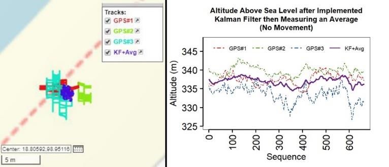
(IJACSA) International Journal of Advanced Computer Science and Applications,
Vol. 12, No. 4, 2021
It is common that the minor discrepancy the device satellite with Arduino Mega 2560 R3 and GY-GPS6MV2 [20].
generated, the more reliable it was. Nevertheless, the GPS modules were divided into three serials and received
acceptable discrepancy of GPS devices has never been signals via Rx Tx pin, as shown in Fig. 1.
determined. Instead, it differed according to the objectives and
the application of each device. For example, ground vehicles' Data were collected by running commands via Arduino
navigation system needed few-meter accuracy, whereas the IDE and then logged into a Serial Monitor. Each round of data
land surveying drone needs centimeter accuracy because the collection lasted approximately 2 – 3 seconds. There were 3
pictures should be in high resolution. When the pixels were sets of data collected. Each set composed of Latitude,
smaller, less discrepancy was essential. Therefore, for Longitude, and True Altitude (the height above mean sea level)
Waypoint Tracking and Stich Image, which needed more collected from each GPS receiver.
precision, Real-Time Kinematic (RTK) devices with more After 30 seconds of GPS sensor calibration, the GPS
accuracy were used instead [11]. receivers then started to collect data from the satellite. Each
After many problems with instability GPS signals were loop started after a 2-second delay since the average time
reported, many inventors have developed algorithms to be used measured before the experiment was 2 seconds.
with such devices to increase their efficiency for the most There were two main scenarios for data collection; one was
satisfying results [12]. Upon further literature reviews, there when the sensors were completely still (no movement), and the
have been many published articles on hardware development other was when the sensors were moving for at least 30
via algorithms. Among those, there were three interesting seconds. All data were later used for average calculation and
experiments that were in accordance with the mentioned Kalman Filter implementation in order to decrease
principle. The first experiment was the estimation and discrepancy, as shown in Table I. The results from all six
improvement of GPS coordinates in UAV to be more stable via methods were analyzed to determine the most efficient method
an algorithm called Kalman Filter (a command set estimating for data stability, while all three GPS receivers were entirely
possible data via variance variables (noise covariance) of still with no sensor movement.
sensors [13]) with GPS and Barometer based on Position-
Velocity-Acceleration model [14]. From this experiment, it
was found that the PVA method using Kalman Filter generated
relevant results for further studies related to Extended Kalman
Filter (the further research of the owner of this experiment).
Kalman Filter was also further developed for more specific
purposes; for example, Extended Kalman Filter (EKF) was
further developed from Standard Kalman Filter to estimate
variant data as Non-Linear [15,16]. The second experiment
presented here was the integration of EFK with small UAV,
UWB (Ultra-Wild Band), cheap MUI devices, and indoor
vision-based sensors [17]. The result of this experiment
showed that the EKF application generated approximately a
10-centimeter discrepancy from actual positions. This result
proved that hardware GPS positions could be improved by
optimizing results via a software algorithm and further
improved efficiency.
Fig. 1. Circuit Diagram Chart for GPS Signal Receiver.
In addition to using Kalman Filter to stabilize GPS devices,
the other interesting method was averaging outcomes from TABLE I. CALCULATION METHODS FOR DATA EFFICIENCY
more than one GPS device for more statistically accurate IMPROVEMENT
results and for the inaccuracy distribution to be nearer to
Normal Distribution compared with using only one GPS device N No
Method Moving
o. Movement
[18]. The third experiment was using Extended Kalman Filter
with several Low-cost GPS receivers to increase the efficiency 1 Implementing Kalman Filter
of GPS devices on UAVs by installing one u-box GPS receiver 2 Measuring for an average
on each arm of the quadrotor, and one more on the center
Implementing Kalman Filter and then
point, totaling five receivers. This experiment showed that the 3
measuring for an average
outcomes were more reliable than using only one GPS
device [19]. Implementing Kalman Filter and then
4 measuring for an average for every 2 to N
term
III. METHODOLOGY
Measuring for an average and then
A. Structure 5
implementing Kalman Filter
For this experiment, two types of equipment were used to Measuring for an average and then
collect data from GPS: a Microcontroller for processing and 6 implementing Kalman Filter for every 2 to N
presenting data and GPS receivers for receiving data from a term
383 | P a g e
www.ijacsa.thesai.org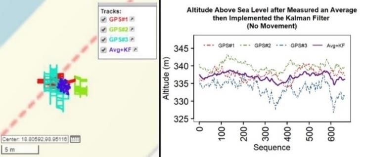
(IJACSA) International Journal of Advanced Computer Science and Applications,
                                                                                                                    Vol. 12, No. 4, 2021

B. Standard Kalman Filter Approach                                        There were two rounds of data collection, one when the
    Kalman Filter is a set of computer commands used to               sensors were completely still and the other when the sensors
predict possible outcomes of linear equations based on                were continually moving. For the one when the sensors were
estimations from Mean Square Error from historical data.              completely still, there were 663 sets of data collected, while for
                                                                      the one when the sensors were.
    This experiment also used Kalman Filter with the same
algorithm as the previous study [21], which consisted of three            The picture on the left of Fig. 2 showed the location of 663
steps: 1) Initialization: initialed the variables used in             sets of GPS data read from all three sensors with no movement
prediction, 2) Prediction: calculated data for the possible           after visualizing on Grafana Application. This data collection
outcomes, and 3) Update: currently collected data for the             lasted 1,982 seconds, or 33 minutes and 2 seconds. On average,
prediction of the next set of data. Prediction and Update             each read took 2.99 seconds.
functioned together recursively for data prediction using                The GPS data read from each of the moving sensors was
Kalman Gain as variables determining the future's possible            shown in the right picture of Fig. 2. This data collection
outcomes would be according to the current data. The                  contained 839 sets of GPS data and lasted 2,326 seconds, 3
equations for Standard Kalman Filter Data Prediction were:            minutes, and 46 seconds. On average, each read took 2.77
Initial ̂       and                                           (1)     seconds.

̂           ̂                                                 (2)          The altitude above sea level read when the sensors were
                                                                      completely still and when they were constantly moving were
                                                              (3)     represented by red, green and blue lines, respectively. On the
                                                                      left of Fig. 3, the range of the sensors with no movement was at
                                                              (4)     16.5 meters, with the lowest at 316.7 meters and the highest at
̂      ̂                ̂                                     (5)     343.2 meters. Meanwhile, the range of the moving sensors was
                                                                      at 39.8 meters, with the lowest at 267.6 meters and the highest
                                                              (6)     at 307.4 meters, as shown on the right of Fig. 3.
     The objective of these equations was to find an estimated            The collected data would then be calculated for the
value of the data at time K, aka ̂ , based on data collected          distribution of data, namely the Maximum, Minimum, Range,
from the current time ( ) according to           (Kalman Gain),       Standard Deviation, Mean Deviation, and Variance, derived
This was a crucial variable that varied directly with data from       from each sensor.
the past (1). Equation (2) and (3) were Prediction State where
                                                                          The distribution of Latitude and Longitude were shown in
roughly estimated data were stored in ̂ (Prior estimate) and
                                                                      Table II, and True Altitude (Altitude Above Sea Level) was
    (Prior error covariance) before being used later in Update,       shown in Table III. However, the experiment with moving
which was related to (4), (5), and (6) to finally yielding results    sensors was not calculated for the distribution of data because
in the estimate called ̂ .                                            the actual position was changed continuously, meaning that all
                         IV. EXPERIMENT                               data could not be used to find the current location's distribution.
    Upon turning on the signal receivers, the calibration took
30 seconds before data collection started. Every collected GPS
data would be displayed on the Serial Monitor of Arduino IDE.
The data collection lasted at least 30 minutes, timed by a time
switch. Every read needed approximately 2 – 3 seconds, and
after which, all collected data were stored for further
calculation.
    The first experiment was to collect GPS data while the
sensors were completely still. This experiment's location was
the open space near the reservoir with no high buildings within
a 100-meter radius from the receivers' position. The experiment         Fig. 2. GPS Positioning of all Three Sensors when the Equipment was
was conducted at around 5.30 pm, during a clear sky with no           Entirely Still (Left) and when the Equipment was Constantly Moving (Right).
visible cloud. The total time spent was 33 minutes and 2
seconds.
    The following experiment was to collect GPS data while
the sensors were continually moving. The location for this
experiment was in the city, surrounded by no higher than 4-
story buildings. The experiment was conducted at around 5.32
pm, during a clear sky with no visible cloud. The GPS
receivers were sticking out from a backpack while the
backpack carrier walked for 2.76km with the average speed at          Fig. 3. Altitude above Sea Level Received from all Three Sensors when the
7 – 8 m/hr, referring to Nike Run Club Application. The total         Equipment was Completely Still (Left) and when the Equipment was Moving
time spent was 41 minutes and 30 seconds.                                                              (Right).

                                                                                                                                 384 | P a g e
                                                        www.ijacsa.thesai.org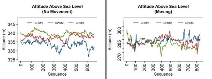
(IJACSA) International Journal of Advanced Computer Science and Applications,
Vol. 12, No. 4, 2021
TABLE II. STATISTICAL DATA OF LATITUDE AND LONGITUDE MEASURED FROM MULTIPLE GPS RECEIVERS WHILE THE RECEIVERS WERE COMPLETELY
STILL
GPS#1 GPS#2 GPS#3
LAT LNG LAT LNG LAT LNG
Max 18.805810 98.951019 18.805807 98.951034 18.805820 98.951011
Min 18.805789 98.950973 18.805782 98.951019 18.805765 98.950981
Range (m) 2.34 5.12 2.78 1.67 6.12 3.34
S.D. 0.0000046 0.0000088 0.0000049 0.0000041 0.0000119 0.0000064
Variance 2.08E-11 7.79E-11 2.39E-11 1.70E-11 1.43E-10 4.05E-11
TABLE III. STATISTICAL DATA OF ALTITUDE ABOVE SEA LEVEL FROM THREE RECEIVERS IN BOTH NON-MOVING AND MOVING CONDITIONS (METER)
No Movement Moving
GPS#1 GPS#2 GPS#3 GPS#1 GPS#2 GPS#3
Max 340.70 343.20 337.50 301.30 299.30 307.40
Min 333.80 336.90 326.70 270.00 267.60 272.30
Range 6.90 6.30 10.80 31.30 31.70 35.10
S.D. 1.47 1.19 2.04 4.65 4.63 3.73
Variance 2.17 1.41 4.17 21.64 21.46 13.89
receivers were used to calculate the averages before
Latitude, Longitude and True Altitude were calculated to implementing Kalman Filter.
improve the stability of data using six methods. From all of the
six methods, there were three interesting methods when applied Even though the Ranges of latitude, Longitude, and True
to all ten scenarios as presented here. Attitude of this method were the same as the first method, this
method's statistical variance was significantly lower. As shown
A. Implement Kalman Filter to Data at a Certain Time and in Fig. 5, the second method's data distribution was remarkably
then Measure the Averages similar to that of the first method, making it hard to distinguish
This method conducted two calculations. The first via observation. From Table V, the variances of the GPS
calculation was implementing Kalman Filter to data from each positions of both methods were slightly different, while the
sensor since it was found in previous studies that Kalman Filter altitudes bore no difference at all at two decimal places.
could lower discrepancy to a certain level. However, the results
were not efficient enough to stabilize the data [11]. Therefore,
the second calculation for this method aimed to elevate the data
improvement by measuring the averages using (9).
∑
(1)
∑
(8)
∑
(9)
Fig. 4. GPS Positions and Altitude above sea Level Received from all 3 GPS
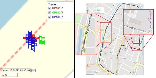
The results from (7), (8), and (9) were the GPS locations Receivers after Implementing Kalman Filter and then Measuring the Averages
when the Equipment was Completely Still.
and altitudes when the sensors were completely still as shown
in Fig. 4.
TABLE IV. STATISTICAL DATA OF LATITUDE, LONGITUDE, AND ALTITUDE
The purple area was the one where Kalman Filter was ABOVE SEA LEVEL FROM THREE RECEIVERS AFTER IMPLEMENTING KALMAN
FILTER AND MEASURING THE AVERAGES WHILE THE SENSORS WERE
implemented before measuring the averages. It was noticeable COMPLETELY STILL
that the area was narrower compared to the other three sets of
unprocessed data from three sensors due to the decreased data
distribution. Table IV showed the statistical data with Max 18.805804 98.951013 338.76
significantly decreased deviation compared with unprocessed
Min 18.805785 98.950998 334.44
data in Table II and Table III.
Range (m) 2.11 1.67 4.32
B. Measure the Averages, and then Implement Kalman Filter
S.D. 0.0000041 0.0000035 1.01
This method was similar to the first method, and the
difference was only that each set of data from all three Variance 1.72252E-11 1.24139E-11 1.02
385 | P a g e
www.ijacsa.thesai.org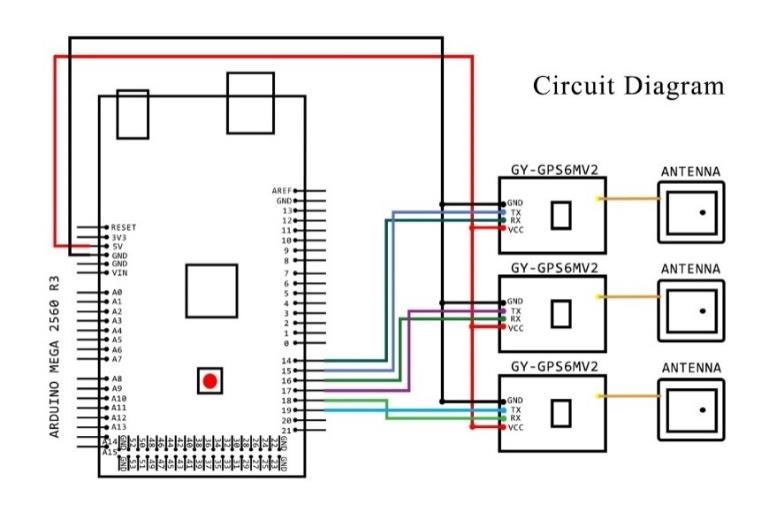
(IJACSA) International Journal of Advanced Computer Science and Applications,
                                                                                                                                 Vol. 12, No. 4, 2021

                                                                                   calculated with this method with average calculation at 2, 3
                                                                                   intervals and from 1 to 663 terms.
                                                                                       For the case that the equipment was constantly moving, this
                                                                                   method calculating for averages from 1, 2, to 663 terms would
                                                                                   not be used. This was due to the fact that, when the Interval of
                                                                                   the averages were increased, the data would start moving
                                                                                   towards the center of the data as shown in Fig. 7 where the
                                                                                   path of data at Interval 1 to the total number at 663 sets for the
                                                                                   case that the equipment was continually moving. The Purple
    Fig. 5. GPS Positions and Altitude above Sea Level from all 3 GPS              Line and the Blue line represented calculations with both
Receivers after Measuring the Averages and then Implementing Kalman Filter         Kalman Filter and Average Measurement. It is evident that
                 when the Equipments were Completely Still.                        when time passed, the path was compressed towards the center
                                                                                   of the data. Therefore, this method was not used for moving
  TABLE V.     STATISTICAL DATA OF LATITUDE, LONGITUDE AND TRUE                    equipment.
  ALTITUDE AFTER MEASURING THE AVERAGES AND THEN IMPLEMENTING
     KALMAN FILTER WHILE THE SENSORS WERE COMPLETELY STILL

Max                 18.805804             98.951013            338.76
Min                 18.805785             98.950997            334.44
Range (m)           2.11                  1.78                 4.32
S.D.                0.0000041             0.0000035            1.01
Variance            1.70901E-11           1.25134E-11          1.02
                                                                                      Fig. 6. GPS Positions and Altitude above Sea Level from all 3 GPS
C. Use the Data to Measure the Averages and then                                      Receivers after Measuring the Averages of Every n Term Interval then
    Implementing Kalman Filter for Every 2 to N Terms                                    Implementing Kalman Filter while Sensors bore no Movement.
    It was found that using GPS data to calculate for averages
before implementing Kalman Filter yielded better results;
therefore, for this third method, every N Term was measured
for averages before Kalman Filter was implemented, N being
the Interval Number of data calculated for averages. For
example, if N = 3, the system would read GPS data 3 times and
then used these three values for calculation. The average
gained from each GPS receiver were then added together and
divided by the number of receivers (3 in this particular case) to
find the average of Multiple Sensors, which were then
implemented with Kalman Filter. This method aimed to
observe the tendency of data in the case that the Interval of
finding averages kept increasing while the GPS receivers bore
no movement.
    Table VI found that data distribution tended to keep
decreasing when N (average Interval) increased. Upon
checking the range of distribution, when Interval equaled 2, 3,
and kept going to the total number (N), it could be seen that for                   Fig. 7. GPS Positions after all Three Sensors were Measured for Averages
every increasing N, the standard deviation decreased and                            and Implemented with Kalman Filter Every N Term, and after Data from all
tended to keep decreasing. The change of the graph's trend was                      Three Sensors were Implemented with Kalman Filter and then Measured for
noticeable in Fig. 6, which showed the comparison of data                                Averages in the Case that the Equipment was Continually Moving.

      TABLE VI.    STATISTICAL DATA OF LATITUDE, LONGITUDE, AND ALTITUDE AFTER MEASURING FOR THE AVERAGES OF EVERY N TERM INTERVAL THEN
                                         IMPLEMENTING KALMAN FILTER WHILE SENSORS BORE NO MOVEMENT

                  Measurement Interval = 2 terms                  Measurement Interval = 3 terms                 Measurement Interval = 1, 2, …, 663terms
                  LAT              LNG                ALT         LAT              LNG              ALT          LAT              LNG               ALT
Max               18.805803        98.951012          338.66      18.805802        98.951011        338.58       18.805803        98.951006         337.62
Min               18.805786        98.950998          334.58      18.805786        98.950998        334.72       18.805796        98.951001         336.56
Range (m)         1.89             1.56               4.08        1.78             1.45             3.86         0.78             0.55              1.06
S.D.              0.0000040        0.0000033          0.98        0.0000038        0.0000031        0.95         0.0000011        0.0000011         0.29
Variance          1.57E-11         1.07E-11           0.96        1.43E-11         9.48E-12         0.91         1.28E-12         1.21E-12          0.08

                                                                                                                                              386 | P a g e
                                                                  www.ijacsa.thesai.org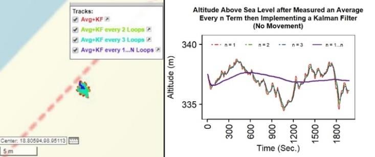
(IJACSA) International Journal of Advanced Computer Science and Applications,
                                                                                                                    Vol. 12, No. 4, 2021

                                                                           only one method. From Table VII, in the case that Kalman
                       V. RESULT ANALYSIS                                  Filter was implemented before average measuring with non-
     This experiment demonstrated three methods used to lower              moving equipment, it was found that the Ranges of Latitude,
the distribution of data: 1) Implementing Kalman Filter,                   Longitude, and Altitude for this particular method was
2) Finding Averages and 3) Implementing Kalman Filter and                  narrower at 0.23, 0.55, and 0.38 meters, respectively, when
Finding Averages. From the distribution data shown in                      compared with the method with average measuring only. The
Table VII, the least effective method was solely implementing              tendency of lower data distribution was similar for the case
Kalman Filter. The Standard Deviations of GPS Coordinates                  with moving equipment. For the case with non-moving
(Latitude, Longitude) while the GPS receivers were completely              equipment, using more loops to find data averages yielded
still were decreased by 3.39% and 10.7% on average; whereas                more stability. As time passed, every increasing Interval of
the Standard Deviations of True Altitude were decreased by                 average finding statistically significantly lowered the
2.99% and 6.23% for the non-moving equipment and the                       distribution of data. However, the method of finding averages
moving equipment, respectively. Even though it is evident that             before implementing Kalman Filter yielded more stable data
Kalman Filter could help reduce the distribution of data, but its          distribution when N increased compared to implementing
efficiency was too low to be used with projects which needed               Kalman Filter before finding averages. However, statistics
data stabilization, as previously mentioned in earlier studies             showed that when the equipment was entirely still, finding
regarding Kalman Filter [11].                                              averages and then implementing Kalman Filter at any N, the
                                                                           variances were so close to solely implementing Kalman Filter
    Next up was the method where data were used to find                    at any N that the differences were unnoticeable with bare eyes.
averages. This method significantly increased the stability and            Similarly, with moving equipment, data measuring for
decreased data distribution better than the one implementing               averages before implementing Kalman Filter yielded slightly
only Kalman Filter. The Standard Deviation of Latitude and                 higher variances compared to the other method; therefore,
Longitude for non-moving equipment were decreased by 49%                   hardly bearing any effect upon implementation. Nevertheless,
and 75.21%. The Standard Deviation of True Altitude for non-               the method of implementing Kalman Filter together with
moving equipment and moving equipment was decreased by                     measuring for averages with increasing loops was incompatible
65.45% and 40.94%, respectively. They were resulting in more               with the case of moving equipment since the average of a
stability compared to the method solely implementing Kalman                specific position at any time required data from that particular
Filter.                                                                    position; otherwise, the results would be incorrect as shown in
    Implementing both Kalman Filter and average measuring to               Picture 7. For example, every loop required 10 meters of a
improve data stability could be further divided into four sub-             straight line. If data from the current position were combined
methods: 1) They were using results after implementing                     with data from the previous position 10 meters away and
Kalman Filter to find averages, 2) using Kalman Filter results             calculated for an average, the result would be the 5-meter
to find averages of every data from 1 to N loop, 3) using data             average between these two positions, which was 5 meters away
after finding averages to implement Kalman Filter, and 4)                  from where it was supposed to be. This was the reason why
using the averages of every data from 1 to N loop to implement             calculations with average loops were unsuitable to be used with
Kalman Filter. Based on all these sub-methods statistical data,            moving equipment to lower the variances of GPS positioning
it was found that implementing Kalman Filter and average                   data.
findings could better stabilize the data compared to applying

                           TABLE VII.   STANDARD DEVIATION AND RANGE OF DATA FROM EACH CALCULATION METHOD

                                  No Movement                                                                      Moving
Method                            GPS Coordinate                                    True Altitude                  True Altitude
                                  S.D. (Lat,Lng)              Range (m)             S.D. (m)         Range (m)     S.D. (m)        Range (m)
Raw data                          0.0000084, 0.0000159        6.12, 6.78            3.01             16.50         4.66            39.80
KF                                0.0000082, 0.0000156        5.67, 6.23            2.97             15.18         4.41            25.44
Find average                      0.0000043, 0.0000039        2.34, 2.22            1.04             4.70          2.75            19.50
KF+Average                        0.0000042, 0.0000035        2.11, 1.67            1.01             4.32          2.59            17.18
KF+Average every 2 terms          0.0000042, 0.0000035        2.11, 1.67            1.01             4.30          -               -
KF+Average every 3 terms          0.0000041, 0.0000035        2.11, 1.67            1.01             4.28          -               -
KF+Average every 1…663 terms      0.0000012, 0.0000011        0.78, 0.55            0.28             0.97          -               -
Average+KF                        0.0000041, 0.0000035        2.11, 1.78            1.01             4.32          2.59            17.18
Average+KF every 2 terms          0.0000040, 0.0000033        1.89, 1.56            0.98             4.08          -               -
Average+KF every 3 terms          0.0000038, 0.0000031        1.78, 1.45            0.95             3.86          -               -
Average+KF every 1…663 terms      0.0000011, 0.0000011        0.78, 0.55            0.29             1.06          -               -

                                                                                                                              387 | P a g e
                                                         www.ijacsa.thesai.org
(IJACSA) International Journal of Advanced Computer Science and Applications,
Vol. 12, No. 4, 2021
VI. CONCLUSIONS [6] K. Feng, J. Li, X. Zhang, X. Zhang, C. Shen, H. Cao, Y. Yang, J. Liu,
“An improved strong tracking cubature Kalman filter for GPS/INS
It can be concluded from this experiment that measuring for integrated navigation systems,” Sensors, vol.18, no. 6, June 2018.
averages together with implementing Standard Kalman Filter [7] B.T.M. Leong, S.M. Low, M.P.L. Ooi, “Low-cost microcontroller-based
to three sets of GY-GPS6MV2 Modules to improve the hover control design of a quadcopter,” Procedia Engineering, vol. 41,
pp. 458 – 464, 2012.
stability of cheap GPS equipment can indeed help reduce the
variances of data both when the equipment is constantly [8] N. Acosta, J. Toloza, “Techniques to improve the GPS precision,”
International Journal of Advanced Computer Science and Applications,
moving and when they are completely still. The most effective vol.3, no. 8, 2012.
method is measuring for averages before implementing [9] D. Sathyamoorthy, S. Shafii, Z. Amin, A. Jusoh, S. Ali, “Evaluation of
Standard Kalman Filter. For the case with non-moving the accuracy of global positioning system (GPS) speed measurement via
equipment, the increasing average loops can lower the GPS simulation,” Defence. S&T Technical Bulletin, vol. 8, no. 2, pp.
variances, whereas, for the case with moving equipment, the 121 – 128, November 2015.
increasing average loops reduce data reliability. Even though [10] M.G. Wing, “Consumer-grade global positioning systems (GPS)
the increasing loops for average measuring help reduce data receiver performance,” Journal of Forestry, vol. 106, pp. 185 – 190, June
2008.
variance, it directly varies with time spent collecting data; in
[11] L. Wang, Z. Li, J. Zhao, K. Zhou, Z. Wang, H. Yuan, “Smart device-
other words, the more loops for average measuring, the more supported BDS/GNSS real-time kinematic positioning for sub-meter-
time needed for data gathering for return output. From the level accuracy in urban location-based services,” Sensors, vol. 16, no. 2,
result, there are limitations of moving measurement. The December 2016.
algorithm will slow down the reding cycle to calculate an [12] G.M. Someswar, T. Rao, D.R. Chigurukota, “Global navigation satellite
average and filter of each reding. That would be the primary systems and their applications,” International Journal of Software and
direction for future research to overcome these limitations. Web Sciences, vol. 3, pp. 17 – 23, 2013.
[13] G. Welch, G. Bishop, An introduction to the Kalman filter. University of
In conclusion, this experiment has proved that integrating North Carolina at Chapel Hill, Department of Computer Science, 1995.
Standard Kalman Filter with average finding for multiple [14] G. Schmitz, T. Alves, R. Henriques, E. Freitas, E. El'Youssef, “A
consumer-grade GPS equipment is another suitable alternative simplified approach to motion estimation in a UAV using two filters,”
for projects that need to reduce variances from GPS equipment IFAC-PapersOnLine, vol. 49, issue. 30, pp. 325 – 330, 2016.
at a lower cost. This innovation can elevate data management [15] L. Ljung, “Asymptotic behavior of the extended Kalman filter as a
with variance through computer commands for technological parameter estimator for linear systems,” IEEE Transactions on
Automatic Control, vol.24, pp. 36 – 50, February 1979.
science and geoinformatics. For example, it can be used with
[16] K. Reif, S. Gunther, E. Yaz, R. Unbehauen, “Stochastic stability of the
the guidance system searching for missing persons, improving discrete-time extended Kalman filter,” IEEE Transactions on Automatic
the small projects with customer-grade sensors, or being used control, vol. 44, pp. 714 – 728, April 1999.
to develop future technology and so on continuously. [17] A. Benini, A. Mancini, S. Longhi, “An imu/uwb/vision-based extended
REFERENCES kalman filter for mini-uav localization in indoor environment using
802.15. 4a wireless sensor network,” Journal of Intelligent & Robotic
[1] S. Kumar, K.B. Moore, “The evolution of global positioning system Systems, vol. 70, pp. 461 – 476, April 2013.
(GPS) technology,” Journal of Science Education and Technology, vol.
11, pp.59–80, March 2002. [18] D.K. Schrader, B.C. Min, E.T. Matson, J.E. Dietz, “Real-time averaging
of position data from multiple GPS receivers,” Measurement, vol. 90,
[2] N. Zhu, J. Marais, D. Bétaille, M. Berbineau, “GNSS position integrity pp. 329 – 337, August 2016.
in urban environments: A review of literature,” IEEE Transactions on
Intelligent Transportation Systems, vol. 19, pp. 2761–2778, January [19] A. Shetty, G.X. Gao, “Measurement Level Integration of Multiple Low-
2018. Cost GPS Receivers for UAVs,” in Proceedings of the 2015
International Technical Meeting of the Institute of Navigation, Dana
[3] J. Park, D. Lee, C. Park, “Implementation of vehicle navigation system Point, CA, USA; pp. 26 – 28, January 2015.
using GNSS, INS, odometer and barometer,” Journal of Positioning,
Navigation, and Timing, vol. 4, pp. 141–150, 2015. [20] I.K. Ibraheem, S.W. Hadi, “Design and Implementation of a Low-Cost
Secure Vehicle Tracking System,” in Proceedings of 2018 International
[4] R.J. Meinhold, N.D. Singpurwalla, “Understanding the Kalman filter,”. Conference on Engineering Technology and their Applications
The American Statistician, vol. 37, No. 2, pp. 123–127, May 1983. (IICETA), Al-Najaf, Iraq, pp. 146 – 150, September 2018.
[5] Z. Li, G. Chang, J. Gao, J. Wang, A. Hernandez, “GPS/UWB/MEMS- [21] P. Singkhamfu, A. Prasompon “The Accuracy Enhancement of
IMU tightly coupled navigation with improved robust Kalman filter,”. Consumer-Grade Global Positioning System (GPS) for Photogrammetric
Advances in Space Research, vol.58, pp. 2424–2434, December 2016. and City Mapping Determinations,” International Journal of Building,
Urban, Interior and Landscape Technology (BUILT), vol.14, pp. 81 –
92, 2019.
388 | P a g e
www.ijacsa.thesai.orgYou can also read