Analysing a built-in advantage in asymmetric darts contests using causal machine learning - arXiv

Analysing a built-in advantage in asymmetric
 darts contests using causal machine learning
 Daniel Goller*

 This version: August 2020

Abstract: We analyse a sequential contest with two players in darts where one of the
contestants enjoys a technical advantage. Using methods from the causal machine learning
literature, we analyse the built-in advantage, which is the first-mover having potentially more
but never less moves. Our empirical findings suggest that the first-mover has an 8.6 percentage
points higher probability to win the match induced by the technical advantage. Contestants with
low performance measures and little experience have the highest built-in advantage. With
regard to the fairness principle that contestants with equal abilities should have equal winning
probabilities, this contest is ex-ante fair in the case of equal built-in advantages for both
competitors and a randomized starting right. Nevertheless, the contest design produces unequal
probabilities of winning for equally skilled contestants because of asymmetries in the built-in
advantage associated with social pressure for contestants competing at home and away.

Keywords: Causal machine learning, heterogeneity, contest design, social pressure, built-in
advantage, incentives, performance, darts
JEL classification: C14, D02, D20, Z20.
Address for correspondence: Daniel Goller,
Swiss Institute for Empirical Economic Research (SEW), University of St. Gallen,
Varnbüelstrasse 14, CH-9000 St. Gallen, Switzerland, Daniel.Goller@unisg.ch.

*
 A previous version of the paper was presented at University of Göttingen, University of St. Gallen, and the YSEM, Zurich.
 Special thanks to the participants, as well as Robert Genthner, Sandro Heiniger, Michael Knaus, Alex Krumer, Michael
 Lechner, Gabriel Okasa, Anthony Strittmatter, and Michael Zimmert for helpful comments and suggestions. The usual
 disclaimer applies.

1 0B Introduction
 Contest designers put a lot of effort in designing contests in various fields. For sports

contests, fairness for the contestants and attractiveness for the spectators are the main

restrictions (Szymanski, 2003; Wright, 2014; Arlegi and Dimitrov, 2020). The main fairness

criterion for contests is fulfilled if equally skilled contestants have equal winning probabilities

(e.g. Arlegi and Dimitrov, 2020). To ensure this, most contest designs balance potential

advantages, e.g. home and away matches within one contest to balance the home advantage.

Hence, many contest studies analyse symmetric contests that are designed to have either a

balanced or no technical advantage but empirically uncover side effects, such as the order of

actions (Ginsberg and Van Ours, 2003) or scheduling effects (Goller and Krumer, 2020).

 In contrast, we investigate the fairness of an unbalanced, one match sequential contest

with two competitors in the sport of darts. This contest has a built-in advantage (BIA) for the

first moving contestant, who has an advantage in potentially more, but never less situations

within a match.1 In this study, we analyse a simple question: Is the two player, sequential contest

with BIA a fair contest, or are there specific groups of individuals who are systematically

disadvantaged by the contest design?

 The outcome of a contest is about human behaviour, and even though behavioural

responses are potentially among the most individual, there is hardly any personalized evidence.

The importance of individual behavioural responses calling for more individualized effects

estimation is demonstrated in the work of González-Díaz, Gossner, and Rogers (2012). They

found large differences of individual ‘critical abilities’ of tennis players affecting the

performance and success. While it is impossible to observe or estimate a true individual effect

1
 Sequential contests with different kinds of advantages are widely present. Examples are legislators giving an advantage, in
 form of patents, to a first moving contestant in a market, job posting committees giving an advantage to specific groups of
 the population in a contest for a job, incumbency advantage in political elections, or in sports contests such as the snooker
 championship or NBA and NHL playoffs.

 1

owing to the unobservable outcomes in situations of non-realized interventions, there is a huge

potential to find or describe those individuals who benefit most or least from some given

treatment, which is the BIA in the contest design. For designing rules for competitions,

identifying the most benefiting group of individuals might help improve contest design in terms

of fairness, attractiveness, or competitive balance. This is especially true if specific groups of

individuals systematically realize differential effects and are therefore (dis-)advantaged by the

contest design.

 The relation of incentives and performance is widely discussed in the literature and is

among the fundamentals in contests (Baumeister, 1984; Rosen; 1986; Ehrenberg and

Bognanno, 1990; Ariely, Gneezy, Loewenstein, and Mazar, 2009). Humans behave differently

in situations with increased level of incentives, which are present in many fields of daily life;

such as job talks, presentations or speeches in the public, competitions and decisions at the

workplace or in sports. Often those situations are subject to higher rewards or reputation that

might increase or decrease the performance of individuals. In darts, social incentives might play

a crucial role, owing to euphoric spectators and the otherwise very standardized environment.

For athletes competing near their hometown the stakes are higher. Having a supporting crowd

around might be motivating, which we call social support from now on. Social pressure is the

counterpart, as being watched can also be a burden inducing pressure.2 The increased focus

magnifies the reputation gained if performing well, as well as the loss of reputation, otherwise.

This is a known phenomenon in the social facilitation literature (e.g. Zajonc, 1965; Butler and

Baumeister, 1998), which is found to have an influence even in cases in which not the athlete,

but only the audience has high expectations (Baumeister, Hamilton, and Tice, 1985; Strauss,

1997).

2
 While social support is supposed to improve performance, social pressure results in worse performance (Zajonc, 1965;
 Baumeister, Hamilton, and Tice, 1985).
 2

This motivated us to analyse differential effects in the BIA on an individualized level, as

well as of the respective groups associated with social incentives and ability in a flexible way.

To the best of our knowledge we are the first to empirically analyse a BIA in an asymmetric

two players sequential contest. This study especially contributes in investigating the fairness of

such a contest with a thorough analysis of the BIA using state-of-the-art methodology.

 This work relies on recent advances in econometric methods made in the emerging Causal

Machine Learning literature. These new methods are more flexible compared to parametric

approaches. Moreover, they can deal flexibly with rich data, which makes some identifying

assumptions more credible, and they are useful for the analysis of heterogeneous treatment

effects.

 For this, we use a dataset from the increasingly popular sports of darts, which offers

several benefits when investigating individual responses. Particular for darts is a friendly but

euphoric atmosphere created by the spectators. Moreover, conditions at different venues are

highly standardized. A noteworthy advantage in comparison to various other sports is that there

is no direct interaction between the contestants, which could lead to problems in assessing

individual performance, otherwise. Furthermore, the outcome is precisely measurable, the

rewards are high enough for competitors to take that task seriously, humans are observed while

performing their usual job (Levitt and List, 2008), clear rules avoid subjective decisions by

referees, and almost no external influences.

 As expected, we found the average effect for the technical advantage of moving first to

deliver an about 8.6 percentage points higher probability to win a match. Despite this advantage,

the contest is ex-ante fair for players with symmetric BIAs and a randomized allocation to be

the first-mover. The contest cannot be regarded as fair in case of systematically differential

BIAs, which is systematic effect heterogeneity associated to specific groups. The empirical

analysis shows equal BIAs for equally skilled contestants, but the personalized effects span

 3

from about -5 to +15 percentage points for individuals with different characteristics showing

that there is a substantial heterogeneity in the effect of the BIA. Those contestants with lower

performance measures and less experience profit most from the BIA. Differential effects are

found in line with the social pressure hypothesis, as contestants playing in a neutral environment

benefit from an 8.8 percentage points higher treatment effect compared to those playing in a

supportive environment. Interestingly, this differential effect in the BIA is found only for the

first-mover player, while the second moving player is not affected by this social pressure.

Therefore, this is not a general home disadvantage but is related to social pressure only for the

first moving contestant. This results in an unfair contest design, since equally skilled contestants

do not necessarily benefit from equal winning probabilities.

 In the following section the related literature is discussed. Section 3 provides an insight

into the setting of darts and details the data used. Section 4 presents the methodological

challenges and the estimation procedures used to obtain the results in Section 5, followed by a

conclusion in Section 6.

2 1B Literature review
 There are few studies on the sport of darts, starting with Tibshirani, Price, and Taylor

(2011) analysing the statistics behind darts and the ways to get the highest expected payoffs.

Liebscher and Kirschstein (2017) predicted winning probabilities for individual players in the

world darts championship. While they implicitly incorporated the BIA in their prediction, they

did not intend to estimate causal effects. Ötting, Deutscher, Langrock, Gehrmann, Schneemann,

and Scholten (2020), and Klein Teeselink, van Loon, van den Assem, and van Dolder (2020)

discovered no or low performance decrements under pressure for professional darts players by

looking at more or less pressure owing to varying importance of situations within a match.

Substantial decrements among youth and amateur players are found by Klein Teeselink et al.

 4

(2020), which might suggest a selection of more choking resistant individuals among

professionals.

 One of the most fundamental relations in contests is the role of incentives on performance,

discussed in the behavioural and psychological (e.g. Baumeister, 1984; Masters, 1992; Butler

and Baumeister, 1998; Ariely et al., 2009) and the economics literature (e.g. Stiglitz, 1976;

Shapiro and Stiglitz, 1984; Rosen, 1986; Prendergast, 1999; Lazear, 2000).3 Several works have

investigated the role of social incentives, for example Cao, Price, and Stone (2011) and Toma

(2017), which used data on basketball and found no effect of pressure on performance when a

team plays at home compared to road games. Other works find this to be a source of pressure

that impacts performance negatively. Ariely et al. (2009) found high social rewards to act

counterproductive for performance in a set of experiments. Harb-Wu and Krumer (2019)

investigated shooting performance in biathlon and found home athletes to miss more shots

compared to athletes from other countries. Furthermore, the authors suggested that performance

decrements are present only for the best ranked quarter of athletes. Despite the direct

psychological effect, there is an indirect effect from public expectations (Baumeister, Hamilton,

and Tice, 1985, Butler and Baumeister, 1998, Strauss, 1997). Furthermore, Baumeister et al.

(1985) and Strauss (1997) found performance decrements among individuals in cases in which

the audience, but not the individual expects success.

 Symmetric contests with either a balanced or no advantage are analysed with regard to

differential effects for specific groups in several works. Ginsburg and Van Ours (2003) found

different winning probabilities in a musical contest depending on the order of actions. Dohmen

(2008) and Harb-Wu and Krumer (2019) reported performance decrements among home

contestants compared to non-home contestants. In other works, the groups of first-movers (e.g.

3
 While there is a general agreement, that a small increase in incentives has a positive effect on performance, economic
 theory, such as the efficient wage hypothesis, suggests that stronger incentives lead to more effort and higher output.
 Behavioural research finds performance decrements under circumstances of increased importance mainly for skill-based
 tasks. As it can be assumed that darts is a skill-based task, we focus on research from this literature.
 5

Apesteguia and Palacios-Huerta, 2010) or the second-movers (e.g. Page and Page, 2007) are

found to have higher winning probabilities than the respective other. Recently, Goller and

Krumer (2020) established differential winning probabilities in home matches for underdog

teams depending on scheduling of the matches. Asymmetric contests, in which certain

contestants are favoured by the contest design, are examined in various theoretical works.

Examples are the role of the incumbency advantage for autocrats’ investment decisions

(Konrad, 2002) or in political campaigns (Meirowitz, 2008), and more generally the influences

of head-starts or handicaps in contests (Kirkegaard, 2012; Segev and Sela, 2014). In a more

general scheme, a BIA is found for relative age effects in youth sports, in which children born

at a certain time of year are favoured by the calendar year system, which groups children for

competitive purposes (for a review, see Musch and Grondin, 2001; for a solution on how

operational research can improve fairness, see Hurley, 2009).

 Using sports data, machine learning methods are up to now almost exclusively used for

prediction tasks, rarely in causal studies for average effects but, to the best of our knowledge,

not yet for the systematic estimation of heterogeneous effects.4 Especially in recent years, a

number of methods have been proposed in the Causal Machine Learning literature for

estimating effect heterogeneity (Athey, Tibshirani, and Wager, 2018; Wager and Athey, 2018;

Lechner, 2018; Zimmert and Lechner, 2019; among others). Machine learning methods (or

statistical learning methods, see e.g. Hastie, Tibshirani, and Friedman, 2009) were implemented

or modified to suit the classical causal framework and developed to become useful in analysing

causal questions (Athey, 2017; Athey and Imbens, 2019). While there is some work establishing

theoretical guarantees (e.g. Chernozhukov et al., 2018; Wager and Athey, 2018; Zimmert and

4
 Examples of prediction tasks are forecasting the winner of the darts world championship (Liebscher and Kirschstein, 2017)
 or predicting the final table in the German soccer Bundesliga (Goller et al., 2018). Average causal effects estimations can
 be found for schedule-related issues in soccer, as in Krumer and Lechner (2018) and Goller and Krumer (2020). Further,
 Faltings, Krumer, and Lechner (2019) used a method from the causal machine learning literature in their work on
 favouritism in the Swiss soccer league but did not find any systematic heterogeneity in their effects.
 6

Lechner, 2019) and simulating the performance of the newly developed estimators (notably

Knaus, Lechner, and Strittmatter, 2020a), empirical applications of those new estimators and

the systematic estimation of heterogeneous effects become increasingly popular (examples are

Davis and Heller, 2017; Cockx, Lechner, and Bollens, 2019; Athey and Wager, 2019; Knaus,

Lechner, and Strittmatter, 2020b).

3 2B Setting and data

3.1 Setting
 8B

 Darts players commit themselves to play in one of the two major federations, the British

Darts Organization (BDO) or the Professional Darts Corporation (PDC). While both federations

hold their own tournaments, the PDC receives more media attention and distributes higher prize

money than the BDO.5 The most important tournaments are the (PDC/BDO) World Darts

Championship held in December and January each year. Additionally, during the year, several

other major tournaments are held in different places. The majors are joined by different minor

tournaments throughout the year, relevant for accumulating ranking relevant prize money and

qualification for the major tournaments. For a full list of tournaments considered in this work,

see Appendix E.

 All BDO and PDC darts tournaments operate under the rules of the Darts Regulation

Authority. Most matches are played in the (best-of-K) legs format, where K is an odd number.

This implies that a player who wins (K+1)/2 legs wins the match. To win a leg, the contestants

must score exactly 501 points and complete with a ‘double’ – a special region on the border of

the darts board in which the score achieved is doubled. The two contestants perform their moves

sequentially; for each move, three darts are to be thrown. Once a player reaches 501 points, the

opponent is not allowed to ‘catch-up’. Therefore, the first-mover in a given leg potentially has

5
 There are also combined tournaments for which the players of BDO and PDC can participate. Further, the players may
 change their affiliation any time.
 7

up to three darts more compared to the non-starting player. Having an odd number of maximum

legs played, the first-mover has a technical advantage for the whole match.

 Before each match the starter is determined in a shootout, which is one dart each player,

with the player closest to the centre of the darts board starting the match. How this challenge of

non-random determination of moving first is solved is discussed in Section 4.2. For a more

formal model the interested reader can refer to Appendix C.

3.2 Data base
 9B

 To investigate the BIA, we use data from the sports of darts. Starting from the year 2009

until 2019, matches from the most important BDO and PDC tournaments were extracted from

the software, dartsforwindows, containing information on match statistics and outcomes. This

resulted in a total of 11,604 matches played by 394 different players.6 Importantly, the variable

of interest, i.e. starting the first leg, as well as the outcome variable, winning the match, is

generated. This is complemented by venue and tournament characteristics, such as prize money,

which is standardized to make it comparable over the studied time period.7 Personal

characteristics of the players, such as nationality, hometown, and date of birth, among others

are collected and utilized to create additional variables. Those contain the age or the number of

years the player has played darts at the time of the respective match, or the distance between

the hometown and the venue. Home and Venue in country of birth variables are created if the

player lives within 100 kilometres of the venue, and is born in that country, respectively.8 Since

matches vary in their potential length, the data base contains the maximum number of legs to

6
 After excluding all matches that included players with less than 5 matches, and few other players whose characteristics were
 missing.
7
 Since prize money in tournament m raises substantially over the years t this is standardized as:
 − ( )
 = ( )−min
 .
 max ( )
8
 The main definition of the variable Home of a radius of 100 kilometres around the venue is chosen to specify the hometown
 as close to the venue as possible, i.e. at a distance that family and supporters can easily accommodate, and to observe
 enough individuals as ‘home contestants’ to have sufficient statistical power. Further, to investigate the robustness
 regarding this decision the radius is varied to 50, 150, and 200 km around the venue.
 8

play (bestoflegs) in the respective match. Finally, (pre-match) performance measures and

players statistics, such as the 3-darts average (cumulated 3 darts score, averaged over all the

matches in the past 2 years), rankings, etc., are added. For the full list of covariates and sources,

the reader can refer to Appendices A and F, respectively.

3.3 Descriptive statistics
 10B

 Table 1: Descriptive Statistics
 (1) (2) (3) (4)
 Variable Mean Starting Player Non-starting Player Diff / SD
 Game Outcomes
 Wins Match 0.50 0.55 0.45 0.10
 Wins First Leg 0.50 0.63 0.37 0.27
 Game Characteristics
 Starts First Leg 0.50 1.00 0.00
 Televised 0.32
 Ranking 0.90
 Tournament
 Prize Money 51145 (79918)
 Prize Money 0.13 (0.25)
 standardized
 Player Characteristics
 3 Darts Average 91.82 (4.53) 91.99 (4.49) 91.65 (4.56) 7.54
 Ranking Last 121.74 (292.77) 113.01 (254.99) 130.47 (326.21) 5.97
 Year
 Accumulated 231.15 (270.17) 238.13 (274.46) 224.17 (265.81) 5.17
 Matches
 Left handed 0.07 0.07 0.07 0.80
 Years Playing 19.97 (9.82) 20.07 (9.79) 19.87 (9.85) 2.05
 Years Playing 11.91 (6.21) 11.90 (6.17) 11.91 (6.25) 0.23
 Professional
 Age 36.54 (9.73) 36.46 (9.63) 36.61 (9.83) 1.57
 Venue in country 0.38 0.38 0.38 0.21
 of birth
 Home 0.08 0.08 0.08 0.36
 Distance to 1410.25 (3271.76) 1422.84 (3307.26) 1397.66 (3241.93) 0.77
 Venue
 Observations 11604 11604 11604

Notes: This table presents average values and standard deviations (in parentheses for non-binary variables) of selected
 variables. In the last column the difference for the outcome variables from starting (2) and non-starting (3) player,
 respectively the standardized difference for the player characteristics is reported. Each observation represents one match.
 Values that are equal for all columns are reported only once.

 The outcome variable under consideration is winning the match and is depicted in the

descriptive statistics presented in Table 1. Further, information is provided by categorising the

players according to the variable of interest, i.e. starting the first leg, in columns (2) and (3).

 9

The difference in the outcome variables for starting and non-starting players can be observed

in column (4). If starting the first leg is determined randomly (instead of performing the

shootout) these numbers would be the average treatment effects. Descriptive evidence that

moving first is subject to selection effects can be observed in the standardized differences (SD)

reported in column (4) for the players characteristics.9 Starting players have on an average a

higher 3-darts average, a better ranking position, and more accumulated matches. For the other

characteristics the standardized difference is low. The full list of variables can be found in Table

A.1 in Appendix A.

4 3B Methodology

4.1 Notation and framework
 11B

 The typical notation for binary treatment effects estimation, following Rubin (1974) is

used. Suppose the outcome obeys the observational rule: = (1) + (1 − ) (0), where

 denotes the treatment status ∈ (0,1) , ( ) the potential outcome under treatment status

d. Furthermore, we define to contain the covariates necessary to account for confounding,

and represents those variables investigated in the heterogeneity analysis.10

 The first estimand of interest is the average treatment effect (ATE), = ( (1) −

 (0)). This represents the average effect for all units on the highest level of aggregation.

Contrarily, the estimand on the lowest aggregation level is the individualized average treatment

effect (IATE), ( ) = ( (1) − (0)| = ). The group average treatment effect (GATE)

represents an intermediate aggregation level according to heterogeneity variables , ( ) =

9
 It is unclear in the literature how large the standardized difference can be to still claim the average of the value of a
 respective variable to be balanced among treated and non-treated. Moreover, this is only an indication for average
 balancing. In this work we were very cautious even with seemingly low SD and took non-random treatment allocation
 seriously, as described in Section 4.2.
10
 In principle, and might contain distinct variables or overlap, partly or completely. In this work is an ad-hoc
 selected subset of , used for the heterogeneity analyses and investigating the hypotheses. Throughout the work, random
 variables are indicated by capital letters and realizations of these random variables by lowercase letters.
 10

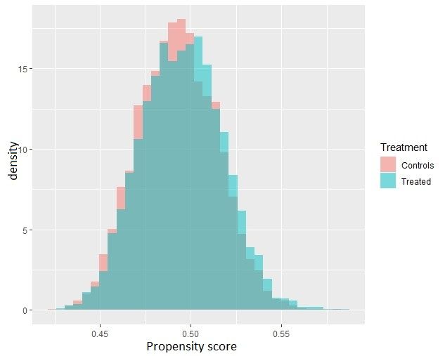
 ( (1) − (0)| = ). Both conditional average treatment effects (CATEs), the GATEs and

IATEs, are useful for detecting heterogeneity among the observed units, which are ‘hidden’ in

ATE estimates.11

 To understand the relationship of those three estimands of interest, integrating the IATEs

over the characteristics of the groups = leads to the GATEs, while integrating over the

characteristics of the entire population results in the ATE. Finally, only one of the potential

outcomes is observable, as a unit can either be treated ( = 1) or non-treated ( = 0); the

other remains counterfactual. In the following section, we shall discuss how to ‘solve’ this

fundamental problem of causal inference (Holland, 1986).

4.2 Identification
 12B

 Most crucial for estimating causal effects is a credible identification strategy. In the case

of randomized treatment assignment, non-treated units can directly be used to construct the

counterfactual outcome. In the underlying case, with non-random treatment assignment, we

impose the following assumptions to identify the estimands of interest based on selection-on-

observables. First, the conditional independence assumption (CIA): (1), (0) ⊥ | = ,

and second, common support (CS): 0 < [ = 1| = ] < 1.

 The first assumption, the CIA, states that the potential outcomes are independent of the

treatment assignment conditional on the confounders. This implies that all variables affecting

both, treatment assignment and outcome, are observed and contained in . The second

assumption, CS, requires that treatment possibilities are bounded away from 0 and 1. This

assumption is testable and of no issue in this work (see Figure A.1 in Appendix B.1).

 At this point, we would like to highlight the two different roles of covariates. First,

covariates (or confounders; ) are required to make the CIA credible. In other words, the

11
 GATE and IATE are special cases of the CATE. The more precise terms are used in this section; throughout this work, the
 terms are used synonymously.
 11

characteristics that are responsible for selection into the treatment status have to be accounted

for to obtain an ‘as-good-as-randomized’ situation. This is necessary to obtain causal treatment

effects, which are free from selection bias. Second, covariates (or heterogeneity variables; )

are used to form groups of observations for which heterogeneous effects are to be estimated.

 In this application, the non-random determination of the treatment, i.e. starting the first

leg, is a result of the shootout to select the starter as already discussed in Section 3.1. The

consequence of this shootout is arguably mainly influenced by the ability of the players and

their experience with this situation. As indicated in Section 3.2, there are two measures of

ability, the previous ranking and the performance in form of the previous average scores

achieved. Experience is measured by the cumulated number of matches played, age, number of

years of playing darts and the number of years played at a professional level. Furthermore, we

control for other variables potentially influencing the selection into treatment as described in

Section 3. Since it is unclear in which (functional) form the potential confounders are most

relevant to account for the selection into treatment, a flexible estimation technique, namely, a

double machine learning approach with non-parametrically estimated nuisance functions,

described in the following section, will be used. Having this set of observed potential

confounders, it is credible that the CIA is satisfied.

4.3 Methods
 13B

 If one considers using a classical linear regression approach to estimate a treatment effect,

there are some implicit assumptions to think about. As already discussed, the conditional

independence assumption is crucial. Further, there are the assumptions of a constant treatment

effect and a linear effect of the confounders on . In most studies, there are neither scientific

nor methodological reasons to motivate these latter assumptions. Therefore, adopting a

methodology not imposing those assumptions is desirable. The upcoming Causal Machine

Learning literature is agnostic about these assumptions.

 12

The growing literature offers several solutions to estimate treatment effects in a flexible

way. For a summary and simulation study covering many of the methods, refer to Knaus,

Lechner, and Strittmatter (2020a). They found four causal machine learning methods with good

performance in all their simulated settings, while other methods were unstable or did not

perform well for estimating the CATE and ATE. Specifically, those are LASSO with covariate

modification and efficiency augmentation (Tian et al., 2014), LASSO with R-Learning (Nie

and Wager, 2017), Causal Forest with local centring (Athey, Tibshirani, and Wager, 2019;

Lechner, 2018), and Random Forest with Double Machine Learning (Chernozhukov et al.,

2018). For this work we chose to use Double Machine Learning, for which we have theoretical

guarantees required for the strategy of our application, e.g. for the ATE (Chernozhukov et al.,

2018) or the CATE (Semenova and Chernozhukov, 2017; Zimmert and Lechner, 2019). To

check the sensitivity of the results being method dependent we chose to additionally perform

the analysis using a Modified Causal Forest (Lechner, 2018).12

 In the following sections, we build on the observation of the two different roles of

covariates. First, the procedure to account for selection into treatment by controlling for

(potential) confounding factors is introduced in Section 4.3.1. Second, two ways how

heterogeneity variables are used to investigate granular treatment effects are described in

Section 4.3.2.

4.3.1 Double machine learning
 25B

 The first stage of the estimation procedure uses the so-called Double Machine Learning

(DML), introduced by Chernozhukov et al. (2018). This approach to overcome the selection

12
 An advantage is the easy implementation of cluster-based sampling, which is helpful in case observations are clustered.
 The potential drawback of the Modified Causal Forest method is efficiency loss owing to the requirement of sample
 splitting for weight-based inference, which can be circumvented by cross-fitting in the Double Machine Learning approach.
 Moreover, it works with only discrete or discretized heterogeneity variables. For a more detailed description the interested
 reader is referred to Lechner (2018) in general, as well as the appendix for a short introduction and the process of its
 implementation in this work.
 13

problem builds on the augmented inverse probability weighting procedure, going back to

Robins, Rotnitzky, and Zhao (1994, 1995):

 � − 1 ( )� (1 − )( − 0 ( ))
 ∗ = 1 ( ) − 0 ( ) + − ,
 ( ) 1 − ( )

 and involves three nuisance parameters. 1 ( ) = ( | = 1, ), modelling the

conditional outcome mean if treated, 0 ( ) = ( | = 0, ), the conditional outcome mean

if not treated and ( ) = ( | ), the conditional probability to be treated.13 This results in

the orthogonal score ( ∗ ), which has various applications. The expected value of the orthogonal

scores, i.e. ( ∗ ), is the average treatment effect. The lowest level of aggregation is obtained

as ( ∗ | = ), while group average treatment effects can be obtained by the expected value

conditional on the groups defined in Z as ( ∗ | = ), which are discussed in detail in Section

4.3.2. The three nuisance parameters in general can be estimated by any well-suited estimation

technique.14

 To overcome the linearity assumption of effects by the confounders on the outcome, the

non-linear and non-parametric Random Forest is used to estimate the nuisance parameters. The

Random Forest algorithm, developed in Breiman (2001), is built as an ensemble of single

Regression Trees, which are to some extent randomly constructed.15 Each Regression Tree

recursively splits the space of covariates into non-overlapping areas to minimize the MSE of

the outcome prediction until it reaches some stopping criteria. The resulting structure is

reminiscent of a rotated tree; one can observe the trunk gradually splitting up into finer

13
 Following Chernozhukov et al. (2018), the nuisance parameters are estimated based on a 2-fold cross-fitting, in which first
 the sample is randomly divided into 2 equally sized folds. In each of the folds, the prediction model is estimated, while in
 the respective hold-out fold, the model is used to predict the nuisance parameters. While no observation is used to predict
 its own nuisance, we can use all observations without running into problems of overfitting.
14
 There are requirements on the rate of convergence of the estimators (depending on level of aggregation, cross-fitting, etc.).
 Those requirements are met for standard regression models, such as OLS and Probit, as well as for specific methods
 coming from the machine learning literature, such as Random Forest or LASSO and others. In this work, the Random
 Forest is used, for which the required rates are given (compare Wager and Walther, 2015).
15
 For each tree 50% of the data are subsampled. To further de-correlate the trees at each split, only a subset of the available
 covariates is randomly chosen.
 14

branches. The averages of the outcomes of those observations falling into the same end-nodes

(so called leaves) provide the predictions of the tree. Combining several of those tree

predictions results in the final predictions of the Random Forest.16 This DML step is to remove

any (potential) confounding issues. The resulting orthogonal score is free from selection effects,

and treatment effects can be constructed at various levels of aggregation.17

4.3.2 Conditional average treatment effects
 26B

 As already mentioned, the scores can be used to directly obtain the average treatment

effect by = ( ∗ ). To estimate effects beneath the average level, the obtained orthogonal

scores from the DML procedure can be used in different ways. Consider first using the Best

Linear Predictor (BLP) framework proposed in Semenova and Chernozhukov (2017). Here, the

orthogonal scores are used as pseudo-outcome in an ordinary least squares regression on

covariates to solve the minimization problem: ̂ = ∑ �∗ � )2 , with � 
 =1( − 

containing a constant and . The fitted values, �( � ) = � ̂ are the best linear predictors of the

IATEs. In fact, � can be replaced by any subset of the covariate space. For example, replacing

it by only a constant leads to the ATE; replacing � by � = ( , ) leads to the GATEs.

Standard errors can be computed as heteroscedasticity robust standard errors, which are valid,

as shown in Semenova and Chernozhukov (2017).18 Once the IATEs are estimated, they can be

analysed in various ways. One possibility is to evaluate the distribution of the effects, to observe

how different the effects are for the range of observations. Chernozhukov, Fernández-Val, and

Luo (2018) suggested the Sorted Effects method, which sorts the individualized effects

according to the effect size, coming with valid confidence intervals. Furthermore, this can be

16
 All the necessary tuning parameters are determined in a data-driven way using cross-validation. For more details on
 Random Forests, the interested reader can refer to the initial study by Breiman (2001) or the book of Hastie, Tibshirani, and
 Friedman (2009).
17
 For a more detailed discussion, the interested reader can refer to Knaus (2020).
18
 In a sensitivity check, we account for potential clustering on the individual contestant level.
 15

used to analyse whether the most and least affected individuals differ according to their

characteristics.

 The discussed method has its strength in analysing the total range of individualized effects

and compactly summarising heterogeneity. The drawback is that an assumption of linearity of

effects is imposed, as one runs quickly into the ‘curse of dimensionality’ with more than few

heterogeneity variables when using non-parametric methods. To investigate specific

hypotheses, involving few dimensions of the covariate space, Zimmert and Lechner (2019), as

well as Fan, Hsu, Lieli, and Zhang (2019), proposed a non-parametric approach to not be

dependent on the linearity assumption of the best linear predictor. The already estimated

orthogonal scores can be used with (few) selected heterogeneity variables in a classical non-

parametric kernel regression as follows:

 �
 ℎ ( − ) 
 
 ∗
 �( ) = �
 ∑ 
 =1 ℎ ( − )
 =1

 With ℎ being a kernel function with bandwidth h, determined by cross validation and

90% undersmoothing, as suggested in Zimmert and Lechner (2019). The drawback of this

procedure is that the dimension of is limited to obtain the required asymptotic guarantees.

 , in this case, includes one or two heterogeneity variables, which is unproblematic from a

theoretical perspective and sufficient to analyse the hypotheses of interest in this work.

5 4B Results

5.1 Average treatment effect
 14B

 The first result of the analysis is the average effect of the BIA for the starting player on

winning the match. Column (1) in Table 2 shows the average treatment effect. The effect of the

technical advantage with 0.0865 is large and precise enough to be statistically different from

zero. The average effect for the starting contestants, therefore, amounts to 8.65 percentage

 16

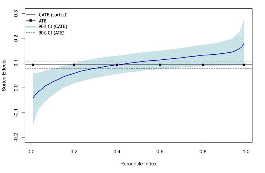
points higher winning probability for the match. This effect is in line with what we would expect

owing to the technical advantage implicit in the contest design.

 Table 2: Base results - best linear predictors
 (1) (2) (3) (4)
 ATE Home Country of birth All
 Intercept 0.0865*** 0.0939*** 0.0853*** 0.0143
 (0.0089) (0.0093) (0.0112) (0.2406)
 Home -0.0885*** -0.0987***
 (0.0323) (0.0347)
 Venue in country of 0.0032 0.0248
 birth (0.0184) (0.0199)
 Prize money -0.0736*
 standardized (0.0488)
 Ranking 0.0000
 (0.0000)
 3-darts average 0.0009
 (0.0026)
 Acc. matches -0.0001
 (0.0000)
 Years playing -0.0016
 (0.0016)
 Years prof. -0.0026
 (0.0024)
 Age 0.0020
 (0.0016)
 Best of legs 0.0011
 (0.0020)
 Observations 11604 11604 11604 11604
 Notes: Best linear prediction as described in Semenova and Chernozhukov (2017); heteroscedasticity robust
 standard error in parentheses. Home is defined as the hometown of the contestant being in the radius of
 100km to the venue. *, **, and *** represent statistical significance at the 10, 5, and 1% level,
 respectively.

 While this is a sizeable effect, it would be interesting to note the kind of players that may

profit more or less from this advantage. To analyse this, we look into more granular effects in

the following sections.

5.2 Individualized average effects
 15B

 Starting on the most granular level, we see in Figure 1 the individualized average

treatment effects for the BIA sorted in size. The solid black line represents the average treatment

effect with the dotted black lines being its confidence intervals. The solid blue line represents

the sorted individualized effects, accompanied by the shaded blue confidence intervals.

 17

Figure 1: Sorted Effects

 Notes: Sorted Effects. 999 (weighted) bootstrap replications. Bias corrected. The blue line represents the
 sorted Conditional Average Treatment Effects accompanied by the shaded 90% confidence interval.
 The black line with squares represents the ATE, accompanied by the dashed line representing the 90%
 confidence interval.

 While most of the players have positive effects, there are also negative point estimates

for specific players. For those players, the technical advantage might not be an actual advantage,

even though this is not backed by statistical confidence. In total the individualized effects range

from around –5 to +15 percentage points, suggesting that there is some heterogeneity in the

effect.

 A comparison of the 10% most affected (highest treatment effect) to the 10% least

affected (lowest treatment effect) individuals in selected characteristics can be found in Table

3. This helps to evaluate the differences in specific characteristics for those with the highest and

lowest treatment effects. The estimate represents the difference in the characteristics of the most

and least affected. Joint p-values in contrast to the ‘usual’ p-values account for testing the

estimates of, in this case, 10 tests (for more details the interested reader is referred to

Chernozhukov, Fernández-Val, and Luo, 2018).

 18

Table 3: Difference in characteristics of 10% most and least affected groups
 Characteristics Estimate Joint p-value
 p-value
 Ranking 360.89 (109.66) 0.05 0.00
 3-darts average -5.54 (1.79) 0.07 0.00
 Acc. Matches -488.31 (96.48) 0.00 0.00
 Years playing -13.13 (3.78) 0.03 0.00
 Years prof. -11.34 (2.38) 0.00 0.00
 Age -6.87 (4.05) 0.66 0.05
 Venue in country of birth 0.05 (0.21) 1.00 0.40
 Home -0.49 (0.13) 0.02 0.00
 Prize money standardized -0.28 (0.09) 0.09 0.00
 Best of legs -2.54 (2.62) 0.98 0.17
 Notes: Bias corrected, 999 (weighted) bootstrap replications. Joint p-values account for the
 simultaneous inference conducted for all (10) differences of variables. The estimate is the
 difference in the characteristics for the most affected (highest) minus the least affected (lowest
 treatment effect).

 In general, the most affected, i.e. those with the highest realization of the technical

advantage, have lower performance measures, less experience, competing away from home,

and in tournaments with lower prize money, compared to the least affected. A clearly

insignificant estimate can be found for age, which is arguably the worst proxy available for

experience. Furthermore, only home as defined as the hometown being within a radius of 100km

to the tournament venue seems to be differently allocated, while being born in the country

(Venue in country of birth) of the venue is almost equally frequent among most and least

affected.

5.3 Group average treatment effects
 16B

 Now we turn to investigating more specific effect heterogeneities. Two group effects are

investigated: First, in Section 5.3.1, we analyse if there are differential effects in the BIA

associated with the ability of the contestants. Second, we evaluate in Section 5.3.2 whether,

motivated by the social pressure hypothesis, there are differential effects associated to

competitors performing near their hometown.

 19

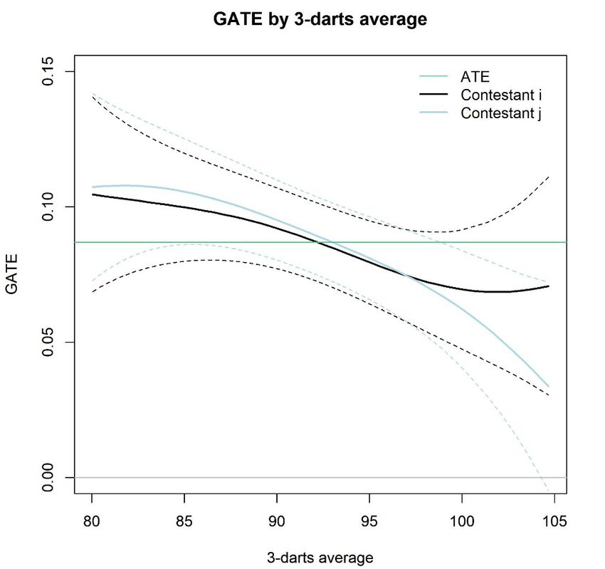
5.3.1 Ability
 27B

 A contest is fair if equally skilled contestants have equal winning probabilities. To

discover if the BIA differs for equally skilled contestants on any level of ability, we therefore

analysed the BIA of the first moving player (contestant i) associated with both competitors’

ability (of i and j). As already discussed, our preferred measure of ability is the performance

measure 3-darts average.

 Figure 2: Built-in advantage of starting contestant by ability

 Notes: The broken lines represent the 90% confidence intervals. Contestant i is the
 starting contestant, j the opponent.

 In general, Figure 2 shows the GATEs to be smaller for higher ability athletes, in line

with the results in Table 3. However, both contestants’ GATEs are close to each other for every

value of the 3-darts average. In other words, there is no evidence that the BIAs are different for

equally skilled contestants. Note that, especially for low and high 3-darts average, there are

fewer observations, resulting in larger confidence intervals.

 20

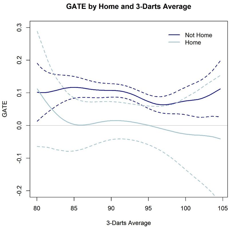
5.3.2 Social incentives
 28B

 We observe in Table 3 that those with the highest treatment effects are rather competing

away from home, with an estimated difference of -0.49, compared to those with the lowest

treatment effects. Investigating this more specifically, the group average effects are shown in

Table 2. Column (2) presents the effect associated with competing at home (-0.0885) relative

to those performing not at home. The technical advantage therefore, exists only for the group

of individuals not performing at home (0.0939), and close to zero for those performing at home.

The diminished winning probability of about 8.8 percentage points for the group of contestants

performing in a friendly environment with support, i.e. at home, is in line with the social

pressure and contrary to the social support hypothesis, as found in Dohmen (2008) and Harb-

Wu and Krumer (2019).19 No substantial difference is found for the group of competitors born

in the same country as the venues’ country (0.0032, column (3) in Table 2). This indicates that

the differential effect associated with competing at home can be attributed to social pressure

from the audience, while there is no difference in the effect associated with the audience

cheering for their compatriots.

 Table 4: Social pressure vs. home (dis-)advantage
 (1) (2) (3) (4)
 ATE Home (i) Home (j) Home (i & j)
 Intercept 0.0865*** 0.0939*** 0.0852*** 0.0926***
 (0.0089) (0.0093) (0.0093) (0.0097)
 Home -0.0885*** -0.0887***
 (Contestant i) (0.0323) (0.0323)
 Home 0.0144 0.0168
 (Contestant j) (0.0323) (0.0323)
 Observations 11604 11604 11604 11604
 Notes: Best linear prediction as described in Semenova and Chernozhukov (2017). Heteroscedasticity
 robust standard error in parentheses. Home is defined as the hometown of the contestant being in the
 radius of 100km to the venue. Contestant i is the starting contestant, j is the opponent. *, **, and ***
 represent statistical significance at the 10, 5, and 1% level, respectively.

19
 Changing the definition of home in terms of a different radius around the venue can be found in Table A.2 in Appendix
 B.3. For a narrower definition of home contestants, the associated effect is larger, while the associated effect decreases if
 defining contestants’ farther away from the venue as home contestants. This supports the general conclusion outlined
 previously.
 21

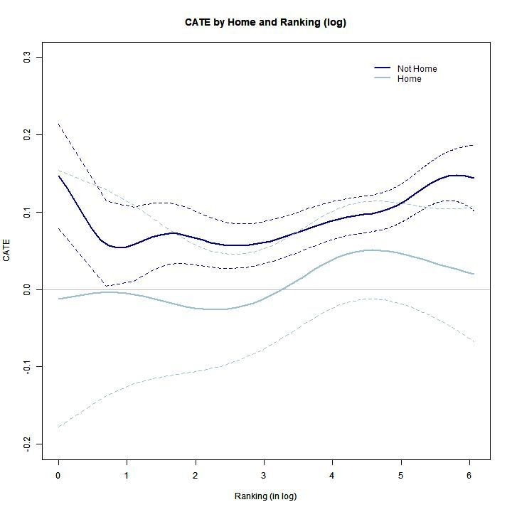
Interestingly, there is no differential effect for the second moving contestant (j) to be

affected by social pressure or any type of home (dis-)advantage, as seen in Table 4. Columns

(1) and (2) are equivalent to those presented in Table 2; columns (3) and (4) show the

differential effect for non-starting contestants associated to competing in a venue near their

hometown. In other words, competing in a friendly environment has no (negative) effect on the

BIA for non-starting contestants. Therefore, there is no evidence for a general home (dis-

)advantage, but evidence in line with social pressure for those starting the match.

 On the contrary, an analogy with the finding of Harb-Wu and Krumer (2019), that the

effect is driven by those athletes in the top quartile of the ability distribution, cannot be

confirmed.

 Figure 3: Differential built-in advantage by home and ability

 Notes: The dark blue line represents the GATEs for contestants not home, the light
 blue line for contestants performing at home. The broken lines represent the 90%
 confidence intervals.

 22

Figure 3 displays the treatment effect for the starter associated with performing at home

or not at home with respect to the 3-darts average, the most accurate measure of individual

ability in darts. We discovered that the effect associated with playing at home fluctuates around

the zero effect, while the effect for those playing away from home is always above. Especially

for the boundaries of the figure, i.e. low and high 3-darts average, there are less observations;

therefore, the estimates become imprecise. Replacing the 3-darts average by the previous

position of the player in the ranking leads to similar conclusions; the results can be found in

Figure A.2 in Appendix B.2.

5.4 Sensitivity checks
 17B

 To assess the sensitivity of the results being method dependent we chose to additionally

perform the analysis using a Modified Causal Forest (Lechner, 2018). For more details on the

method and implementation the interested reader can refer to Appendix D.

 Table 5: Average and Group Average Effects, MCF
 Effects Estimate Standard Error t- value p- value
 ATE 0.0838 0.0147 5.70 0.00
 GATE (home=0) 0.0911 0.0151 6.03 0.00
 GATE (home=1) 0.0038 0.0357 0.11 0.91
 Difference 0.0873 0.0353 2.47 0.01
 With sample-based clustering
 ATE 0.0872 0.0152 5.74 0.00
 GATE (home=0) 0.0931 0.0155 6.01 0.00
 GATE (home=1) 0.0225 0.0365 0.62 0.54
 Difference 0.0706 0.0363 1.94 0.05
Notes: Average Treatment Effect (ATE) and Group Average Treatment Effects (GATE), associated with performing in a
 venue near the hometown (home=1) and not near the hometown (home=0). Home is defined as performing at a tournament
 venue that is within a radius of 100km to the hometown of the athlete. Estimated using a Modified Causal Forest. Inference
 is conducted as weight-based inference. In the lower part of the table, effects are estimated using sample-based clustering
 on the individual player level; 1000 Trees with 50% subsampling rate and the minimum leave size in each tree equals 2.

 All estimated effects are in a comparable range to the estimates in the previous sections.

In addition, the conclusions drawn hold in general. Table 5 shows the ATE estimate, as well as

the GATE associated with performing at home resulting from the Modified Causal Forest

estimation. Further, in the lower part of the table, we repeated the estimation but accounted for

 23

contestant specific clusters. For both estimations, we found a large differential effect associated

to performing at home.

 For the ability measure, 3-darts average, the pattern is in line with the findings from

Section 5.3.1. In Figure A.3 in Appendix B.4 we observe lower GATEs for higher 3-darts

averages of the starting contestant (i) and the opponent (j). Especially, for equal levels of ability

the GATEs are similar. We can therefore conclude that the BIA is symmetric for equally skilled

contestants. Note that, since the 3-darts average is discretized to form groups of roughly equal

numbers of observation in each group, we can see that especially for low and high 3-darts

averages there are less observations. In conclusion, this conceptually different method produces

similar results, providing some evidence that the results presented in the previous sections are

robust.

 Table 6: Base results - best linear predictors, sensitivity to clustering
 (1) (2) (3) (4)
 ATE Home Country of birth All
 Intercept 0.0875*** 0.0948*** 0.0863*** -0.0104
 (0.0095) (0.0100) (0.0120) (0.2316)
 Home -0.0878*** -0.0968***
 (0.0338) (0.0359)
 Venue in country of 0.0030 0.0238
 birth (0.0214) (0.0225)
 Prize money -0.0936*
 standardized (0.0488)
 Ranking 0.0000
 (0.0001)
 3-darts average 0.0011
 (0.0025)
 Acc. matches -0.0001
 (0.0001)
 Years playing -0.0016
 (0.0016)
 Years prof. -0.0024
 (0.0019)
 Age 0.0019
 (0.0016)
 Best of legs 0.0011
 (0.0018)
 Observations 11604 11604 11604 11604
 Notes: Best linear prediction as described in Semenova and Chernozhukov (2017); cluster-based sampling
 and clustered standard errors on the individual level in parentheses. Home is defined as the hometown of
 the contestant being in the radius of 100km to the venue. *, **, and *** represent statistical significance
 at the 10, 5, and 1% level, respectively.

 24

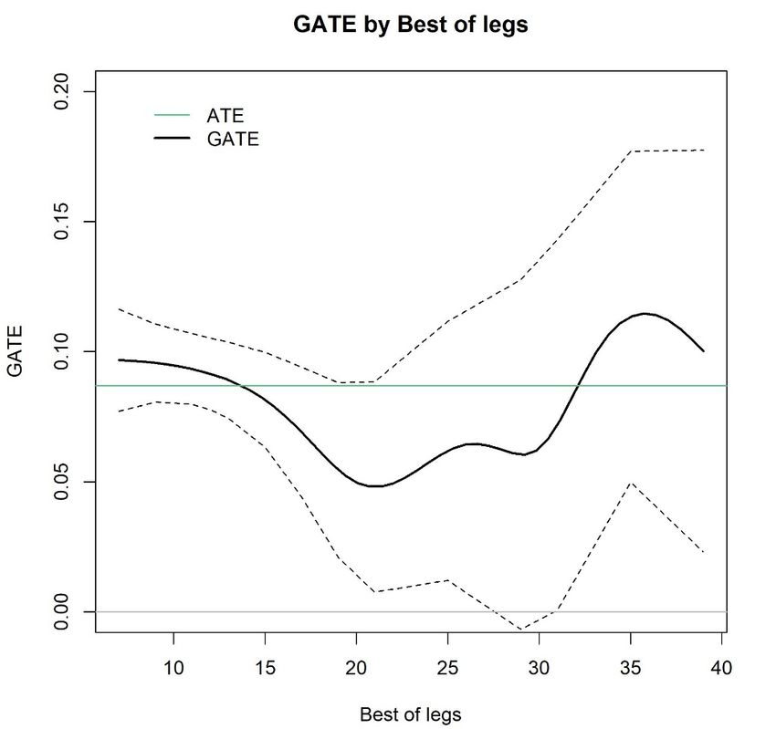
Accounting for potential contestant specific clusters, the best linear prediction results

from Table 2 are replicated with cluster-based sampling for the nuisance estimation, as well as

clustered standard errors on the individual level in Table 6. While standard errors are slightly

higher, we find the conclusions drawn previously are valid.

5.5 Discussion
 18B

 A contest design in which one group systematically realizes differential BIAs is unfair.

Especially when home contestants are affected, the competition design must be reconsidered

and changed to have more fair and interesting contests.

 Figure 4: BIA by maximum number of legs

 Notes: The GATE is shown as solid black line; the broken lines represent the 90%
 confidence intervals. The green line represents the ATE.

 A potential idea is to increase the length of the contest, such that the BIA decreases. While

that looks like a neat idea in theory, we cannot provide clear evidence for it. Figure 4 provides

the BIA associated to the number of maximum legs to play in a match.

 25

The GATE fluctuates around the average effect, with no clear tendency towards lower or

no BIA for longer matches. A second option is to remove the technical advantage from the

contest design in form of even numbers of maximum legs to play, as for example, in tennis

tournaments.20 Further, Cohen-Zada, Krumer, and Shapir (2018) found that the order of serves

in tennis tiebreak, which is the ABBA sequence, does not provide any advantage to any of the

players. Adopting a similar structure might help to improve the fairness in darts contests.

6 5B Conclusion
 The study discovered an average effect of about 8.6 percentage points higher winning

probability induced by the BIA in the sequential darts contest with two players. Having a

randomized allocation of being the first-mover for equally skilled contestants, the contest is fair

for contestants with symmetric potential BIAs. While we found non-differential BIAs for

equally skilled contestants, the personalized point estimates suggested substantial heterogeneity

in the effect, ranging from about -5 to +15 percentage points with athletes having more

experience and better performance measures to benefit least. In addition, estimated differential

effects were in line with the social pressure hypothesis as found in previous works, especially

in the behavioural economics literature. For the group of individuals competing in a friendly

environment, the BIA was lower compared to those competing on neutral grounds, which was

in line with the works of Dohmen (2008) and Harb-Wu and Krumer (2019) among others. This

leads to not necessarily equal winning probabilities for contestants with equal abilities, and

therefore, to an unfair contest.

 For designing contests, the heterogeneous nature of the BIA in such types of contests

should be considered to not unintentionally favour specific groups of contestants. Especially if

20
 Another potential idea to resolve the BIA is to give the respective second-mover the chance to catch-up in case the starter of
 the leg finishes the leg.

 26

fairness is a precondition for a contest, the presented findings should be taken into account.

Despite fairness issues, local athletes might be important for the attractiveness of the contest.

Introducing a fairer contest design may, therefore, improve the attractiveness as well. We did

not find any evidence that an increase in the maximum length for a match leads to diminished

BIAs, so the suggestion would be to change the design of the contest, such that there is no BIA

for any contestant. Furthermore, the findings are of interest to individuals performing in

situations of increased importance, either contestants in tournaments or in daily life situations.

While preparing for those situations, one should put more emphasis on mental training.

 Another insight from this study is that Causal Machine Learning is highly valuable for

empirical studies. It enables us to provide a more complete picture of particular effects under

investigation, as well as a way to investigate specific hypotheses in a flexible way. Furthermore,

the two steps of removing potential selection bias and estimating treatment effects offers an

intuitive, flexible, and robust way to improve credibility of empirical research.

 Finally, we call for more, fine granular investigations in contest designs, particularly in

situations in which there are potentially multiple incentives observable (and distinguishable).

Since we only have data on male professional players, we encourage further studies to analyse

how the BIA affects women, as well as youth and amateur players in darts or other asymmetric

contests. Furthermore, in future studies, the limitations of audience presence owing to the

current corona pandemic could be used to analyse the BIA, without the direct influence coming

from the audience. Methods from the Causal Machine Learning toolbox appear to be especially

useful for this and should be considered for further empirical analyses.

6B References
Apesteguia, J., & Palacios-Huerta, I. (2010). Psychological pressure in competitive environments: Evidence from
 a randomized natural experiment. American Economic Review, 100(5), 2548-2564.
Ariely, D., Gneezy, U., Loewenstein, G., & Mazar, N. (2009). Large Stakes and Big Mistakes. The Review of
 Economic Studies, 76(2), 451-469.

 27