Are Central Banks' Monetary Policies the Future of Housing Affordability Solutions
←
→
Page content transcription
If your browser does not render page correctly, please read the page content below
Article
Are Central Banks’ Monetary Policies the Future of Housing
Affordability Solutions
Chung Yim Yiu

                                         Department of Property, University of Auckland Business School, Auckland 1010, New Zealand;
                                         edward.yiu@auckland.ac.nz

                                         Abstract: Housing affordability is one of the major social problems in many countries, with some ad-
                                         vocates urging governments to provide more accessible mortgages to facilitate more homeownership.
                                         However, in recent decades more and more evidence has shown that unaffordable housing is the
                                         consequence of monetary policy. Most of the previous empirical studies have been based on econo-
                                         metric analyses, which make it hard to eliminate potential endogeneity biases. This cross-country
                                         study exploited the two global interest rate shocks as quasi-experiments to test the impacts and
                                         causality of monetary policy (taking real interest rates as a proxy) on house prices. Global central
                                         banks’ synchronized reduction in interest rates after the outbreak of the COVID-19 pandemic in
                                         2020 and then the global synchronized increase in interest rates after the global inflation crisis in
                                         2022 provided both a treatment and a treatment reversal to test the monetary policy hypothesis. The
                                         stylized facts vividly reveal the negative association between interest rate changes and house price
                                         changes in many countries. This study further conducted a ten-country panel regression analysis to
                                         test the hypothesis. The results confirmed that, after controlling for GDP growth and unemployment
                                         factors, the change in real interest rate imposed a negative effect on house price growth rates. The
                                         key practical implication of this study pinpoints the mal-prescription of harnessing monetary policy
                                         to solve housing affordability issues, as it can distort housing market dynamics.

                                         Keywords: monetary policy; real interest rate; COVID-19; global interest rate shocks; global house prices

Citation: Yiu, C.Y. Are Central Banks’
                                         1. Introduction
Monetary Policies the Future of
Housing Affordability Solutions.              With the dramatic escalation in house prices much faster than household incomes in
Urban Sci. 2023, 7, 18. https://         many countries in the past decades, housing affordability has become one of the major
doi.org/10.3390/urbansci7010018          social problems globally. Numerous research studies have been conducted on the adverse
                                         impacts of housing affordability crises on households and society at large [1–3], especially
Academic Editor: Luis
                                         on young people [4,5]. It has been put on the top priority agenda of policy makers in many
Hernández-Callejo
                                         countries, but almost all of them have focused on increasing land and social housing supply
Received: 23 December 2022               or deregulating urban planning restrictions to facilitate more private housing supply [6–8].
Revised: 24 January 2023                 Unfortunately, after many years’ and many countries’ efforts toward increasing housing
Accepted: 31 January 2023                supply, the global housing affordability crisis does not seem to be resolved, but rather has
Published: 2 February 2023               been heightened to alarming proportions [9]. For example, a general deteriorating trend
                                         was found in the global housing affordability crisis based on a sample of 200 cities.
                                              Some empirical studies, such as that of Fingleton (2008) [10], have found that simply
                                         increasing supply may not be sufficient to reduce house prices as demand factors play a role.
Copyright:   © 2023 by the author.
                                         Borgersen (2022) [11] also found that supply of social housing caused higher house prices
Licensee MDPI, Basel, Switzerland.
This article is an open access article
                                         and crowded out those who were not included in the social housing schemes. Thus, Raisner
distributed under the terms and
                                         and Bracken (2022) [12] of the World Economic Forum contended that providing ‘more
conditions of the Creative Commons
                                         mortgages for homebuyers’, among others, is the solution to the global housing affordability
Attribution (CC BY) license (https://    problem in the future. Causa, Woloszko and Leite (2020) [13] agreed that ‘access to mortgage
creativecommons.org/licenses/by/         debt for young household is likely to be one key driver of homeownership for this group,
4.0/).                                   given their relatively low current wealth and income.’ The literature has also confirmed

Urban Sci. 2023, 7, 18. https://doi.org/10.3390/urbansci7010018                                          https://www.mdpi.com/journal/urbansci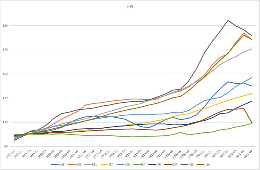
Urban Sci. 2023, 7, 18                                                                                             2 of 18

                         that young households are more sensitive to mortgage policy [14]. Interestingly, a relaxed
                         mortgage policy, such as a lower interest rate or a higher loan-to-value ratio, was found to
                         increase house prices, which rendered housing more unaffordable [15].
                               Ryan-Collins (2019) [16], for instance, raised a contention by asking ‘why can’t you
                         afford a home?’ in his book title. In contrast to the (insufficient) housing supply hypothesis,
                         he put forward a monetary policy hypothesis and argued that it was the ‘unlimited credit
                         and money flows into an inherent finite supply of property that causes rising house prices.’
                               Mian and Sufi (2011) [17] also found empirical evidence on the association between house
                         prices and household borrowing. Numerous pieces of empirical evidence have shown an
                         association between monetary policy, especially interest rate, and house prices [18–27].
                               However, most of these previous empirical studies on this hypothesis have been based
                         on econometric methods, which are subject to endogeneity biases [28,29], such as omitted
                         variable bias, measurement errors and reverse causality [30]. Some studies have applied
                         instrumental variables (IVs) to deal with endogeneity biases, but these have been found to
                         be highly limited [31,32]. IVs are also not appropriate for resolving reverse causality bias.
                               This study focuses on dealing with the reverse causality bias. For example, the causal
                         inference in a panel analysis of monetary policy impacts on house prices can be threatened
                         by reverse causality [33]. The solution to reverse causality, as raised by Kenny (1979) [34], is
                         to establish the temporal precedence of the independent variable to the dependent variable,
                         among other conditions. One of the best solutions to establish temporal precedence is to
                         use experimental trials which can apply interventions to a treatment group and not to a
                         control group [33]. It is hard to conduct real experiments using randomized controlled
                         trials in housing markets, but quasi-experiments on policy changes can be used. This study
                         exploits the global interest rate shocks in the most recent three years as quasi-experiments
                         to eliminate the reverse causality bias and test the monetary policy hypothesis.
                               After the outbreak of the COVID-19 pandemic in 2020, the synchronized actions of
                         cutting interest rates by central bankers provides the first global interest rate shock as the
                         treatment (intervention) to test the monetary policy hypothesis using a quasi-experimental
                         approach. Since the shock was a response of central bankers to deal with the recessionary
                         risks caused by the pandemic, it is an exogenous event to the housing markets.
                               Since February 2022, the outbreak of the Russian–Ukraine war has led the world into a
                         global inflation crisis, triggering a series of global interest rate hikes at different paces and
                         magnitudes. As the global inflation has been largely caused by the surges in fuel prices
                         (oil and natural gas) and food prices due to the war and the supply chain disruptions, the
                         interest rate hikes are also exogenous to the housing market situation.
                               These two global interest rate shocks provide both a treatment and a treatment re-
                         versal [35] to test the cause-and-effect relationship between monetary policy and house
                         prices, which is the novelty of this study. As there are some countries that did not follow
                         the interest rate shocks, they serve as controls for the quasi-experiments. This paper aims
                         to examine the impact and causality of the global interest rate shocks on the global housing
                         market, by empirically studying a ten-country panel regression analysis based on OECD
                         (2022a) [36] data.

                         1.1. From Interest Rate Cuts to Interest Rate Hikes
                              During the COVID-19 period, many cities were locked down and the global supply
                         chains were seriously disrupted, leading to a global recession. With economic activity
                         grinding to a halt globally, central banks ‘implemented unparalleled monetary policies,
                         ultimately lowering their policy rates to historically depressed levels, even below zero’ [37].
                         In 2020, after the outbreak of the pandemic, there were 207 interest rate cuts by central
                         banks [38]. Just in 2020 Q1, there were 73 interest rate cuts by 54 central banks to support
                         the economies and some were even cut to historic lows. Some central banks also relaxed
                         liquidity rules on banks, such as the removal of the loan-to-value ratio restrictions on new
                         mortgages in New Zealand. The global financial markets were flooded with liquidity in
                         this period.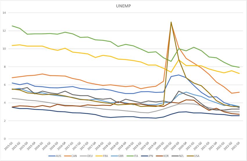
[37]. In 2020, after the outbreak of the pandemic, there were 207 interest rate cuts by central
banks [38]. Just in 2020 Q1, there were 73 interest rate cuts by 54 central banks to support
the economies and some were even cut to historic lows. Some central banks also relaxed
liquidity rules on banks, such as the removal of the loan-to-value ratio restrictions on new
Urban Sci. 2023, 7, 18 mortgages in New Zealand. The global financial markets were flooded with liquidity 3 of in
18
this period.
However, in the wake of a rapid deterioration in inflation, especially after the out-
breakHowever,
of the Russian–Ukraine
in the wake of a rapid war since February
deterioration in2022, many
inflation, central after
especially banksthe started
outbreakin-
creasing interest rates and turned the accommodative monetary
of the Russian–Ukraine war since February 2022, many central banks started increasing policy into a contraction-
ary one.rates
interest In 2022
and Q2, 55 central
turned banks around
the accommodative the world
monetary turned
policy into around to raise interest
a contractionary one. In
rates 62 times, each time not less than 50 basis points [39].
2022 Q2, 55 central banks around the world turned around to raise interest rates In the first three quarters
62 times,of
2022,time
each the world recorded
not less than 50a basis
total of 8190 basis
points points
[39]. In in central
the first three bank interest
quarters rate hikes,
of 2022, the worldand
just counting
recorded theofG10
a total 8190countries alone,intheir
basis points central
central bankbanks raised
interest rateinterest ratesjust
hikes, and by counting
a total of
1850G10
the basis points [40].
countries alone, their central banks raised interest rates by a total of 1850 basis
points [40]. the following ten countries as examples, viz. Australia (AUS), Canada (CAN),
Taking
Germany
Taking (DEU), France (FRA),
the following Great Britain
ten countries (GBR), Italy
as examples, (ITA), Japan
viz. Australia (JAP),
(AUS), South(CAN),
Canada Korea
(KOR), New
Germany Zealand
(DEU), France(NZL),
(FRA),and the United
Great Britain States
(GBR),ofItaly
America
(ITA),(USA),
Japan as shown
(JAP), Southin Figure
Korea
1, mostNew
(KOR), of their short-term
Zealand (NZL),interest
and the rates
United started
Statesfalling rapidly
of America in 2020
(USA), Q2, and
as shown some of
in Figure 1,
them,ofsuch
most theirasshort-term
those in AUS, CAN,
interest GBR,
rates NZLfalling
started and the USA, in
rapidly were
2020 cut to and
Q2, almost
some zero rates.
of them,
ITA and
such JPN were
as those in AUS, theCAN,
exceptions,
GBR, NZLas their
andshort-term
the USA, were interest
cutrates had been
to almost zero close
rates.toITA or
below zero. Then, KOR and NZL raised their interest rates two-quarters
and JPN were the exceptions, as their short-term interest rates had been close to or below earlier than oth-
ers, but
zero. in general,
Then, KOR andmost NZLofraised
themtheir
showed a rebound
interest in short-term
rates two-quarters interest
earlier than rates
others, nobut
later
in
than 2022
general, Q2,of
most except
them ITAshowedand aJPN. The pattern
rebound clearlyinterest
in short-term shows U-shaped
rates no later (downward
than 2022and Q2,
except ITA andshocks
then upward) JPN. The pattern
in global clearlyrates
interest shows U-shaped
within a short(downward
period, with andonethen upward)
in 2020 and
shocks
the otherin in
global
2022.interest rates within a short period, with one in 2020 and the other in 2022.
Figure 1.
Figure 1. Short-term
Short-term interest rates of
interest rates of ten
ten countries
countries from
from 2019
2019 Q1
Q1 to
to 2022
2022 Q3.
Q3. Source:
Source: data
data from
from OECD
OECD
(2022a) [36]. Legend: Australia (AUS), Canada (CAN), Germany (DEU), France (FRA), Great
(2022a) [36]. Legend: Australia (AUS), Canada (CAN), Germany (DEU), France (FRA), Great Britain Britain
(GBR), Italy (ITA), Japan (JAP), South Korea (KOR), New Zealand (NZL), and the United States of
(GBR), Italy (ITA), Japan (JAP), South Korea (KOR), New Zealand (NZL), and the United States of
America (USA).
America (USA).
1.2. From House Price Surges to House Price Falls
Corresponding to the two recent global interest rate shocks, the house prices of many
countries showed strong surges in 2021 and then fell in 2022. For example, the International
House Prices Database reported that 24 out of 25 sampled countries recorded both annual
and quarterly growth in real house prices in 2021 Q3 [41]. Some countries (New Zealand
and Sweden) even recorded unprecedented highs in the annual growth rates of house
prices (25.8% and 17.8%). However, in 2022 Q2 only 10 out of the 25 sampled countries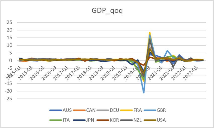
1.2. From House Price Surges to House Price Falls
Corresponding to the two recent global interest rate shocks, the house prices of many
countries showed strong surges in 2021 and then fell in 2022. For example, the Interna-
tional House Prices Database reported that 24 out of 25 sampled countries recorded both
Urban Sci. 2023, 7, 18 annual and quarterly growth in real house prices in 2021 Q3 [41]. Some countries (New 4 of 18
Zealand and Sweden) even recorded unprecedented highs in the annual growth rates of
house prices (25.8% and 17.8%). However, in 2022 Q2 only 10 out of the 25 sampled coun-
tries continued
continued to haveto quarterly
have quarterly
growth.growth.
Based Based on Knight
on Knight Frank’sFrank’s (2021-2022)
(2021-2022) Global
Global House
House Price Index, Figure 2 shows the annual growth rates of the house prices
Price Index, Figure 2 shows the annual growth rates of the house prices of the ten countries. of the ten
countries.
Most Mostindicate
of them of themeither
indicate either a reducing
a reducing rate of increase
rate of increase or evenor even a negative
a negative figure figure
in the
in the annual
annual growthgrowth rate inKOR,
rate in 2022. 2022.for
KOR, for example,
example, showed showed
a plummet a plummet
from thefrom
peak the peak
of rising
of 26.4%
at rising in
at2021
26.4% Q3into2021
a fallQ3 to a fall
of 7.5% of 7.5%
in 2022 in 2022 Q3.
Q3. Similarly, Similarly,
in NZL in NZL
the annual the annual
growth rate of
growthprices
house rate offell
house
fromprices
a peak fell
offrom
25.9% a peak of 25.9%
in 2021 Q2 to ainnegative
2021 Q2 2.0%
to a negative 2.0%ITA
in 2022 Q3. in 2022
and
Q3. ITA and JPN, on the other hand, kept
JPN, on the other hand, kept steady growing trends.steady growing trends.
Figure 2.
Figure 2. Annual
Annual growth
growth rates
rates of house prices
of house prices of
of ten
ten countries
countries from
from 2020
2020 Q1
Q1 to
to 2022
2022 Q3.
Q3. Source:
Source:
data from Knight Frank (2021–2022) [42]. Legend: Australia (AUS), Canada (CAN), Germany (DEU),
data from Knight Frank (2021–2022) [42]. Legend: Australia (AUS), Canada (CAN), Germany (DEU),
France (FRA),
France (FRA),Great
GreatBritain
Britain (GBR),
(GBR), Italy
Italy (ITA),
(ITA), Japan
Japan (JAP),
(JAP), SouthSouth
KoreaKorea
(KOR),(KOR), New Zealand
New Zealand (NZL),
(NZL), and the United States of America (USA).
and the United States of America (USA).
Since these
Since these two
two quasi-experiments
quasi-experiments with global interest
with global interest rate
rate shocks
shocks were
were carried
carried out
out
in different countries, it helps control for the peculiarities of individual countries,
in different countries, it helps control for the peculiarities of individual countries, such such as
differences in planning regulations, land and housing supply constraints,
as differences in planning regulations, land and housing supply constraints, etc. More etc. More im-
portantly, as as
importantly, thethe
interest rate
interest shocks
rate shockshappened
happened almost
almostat at
thethe
same
same time (synchronized),
time (synchronized), it
helps
it eliminate
helps eliminate omitted
omitted variable
variablebias due
bias dueto to
some unobservable
some unobservable temporal
temporalfactors thatthat
factors af-
fected the
affected responses
the responsesofofthe thehousing
housingmarkets
marketsinindifferent
differentcountries
countriesatatdifferent
differenttimes.
times.
This paper
This paper is is organized
organizedas asfollows.
follows.Section
Section2 discusses
2 discusses thethe
study
studygapgapbased on on
based a lit-
a
erature review. Section 3 presents the stylized facts with details
literature review. Section 3 presents the stylized facts with details of the data of the data and the
research design. Section 4 reports the empirical tests’ results. Section 5 discusses the
findings and implications, and Section 6 is the Conclusion.
2. Literature Review
There have already been many theoretical and empirical studies on the impacts of
monetary policy on house prices, but many economists and politicians still disagree about
the role that monetary policies, such as interest rates policy, play in causing house price
booms and busts, probably because almost all the previous studies have not been based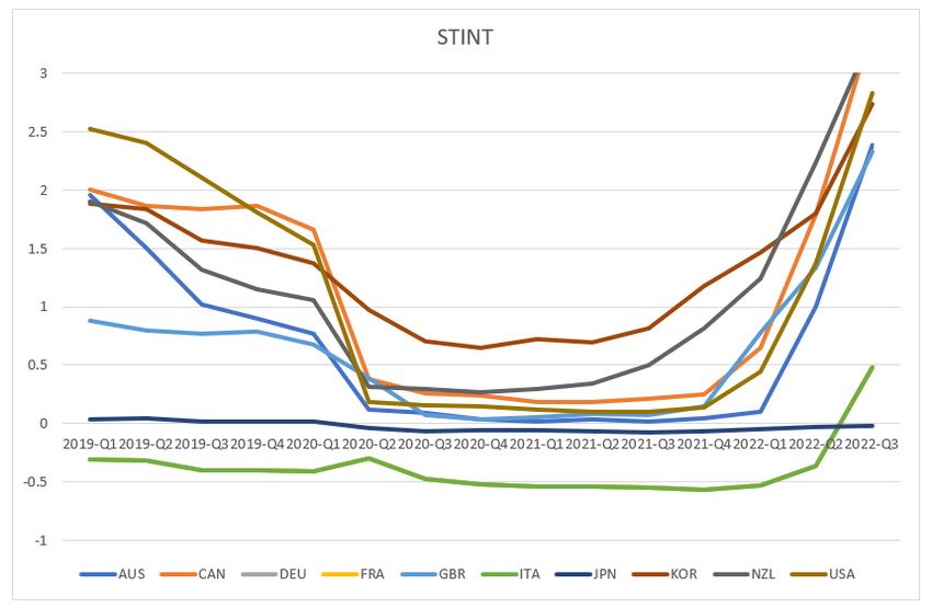
Urban Sci. 2023, 7, 18                                                                                             5 of 18

                         on experiments, and monetary policy can include many tools. For example, Kuttner
                         (2013: 2) [43] reviewed the standard economic theories (such as those in [44,45]) which
                         explain why interest rate changes house values (or the value of any long-lived asset), and
                         contended that interest rate alone could not explain the magnitude of house price changes,
                         and instead it was the overall monetary policy, such as a loosening of credit conditions,
                         plausibly caused by financial innovation (e.g. securitization), and a relaxation of lending
                         standards that caused asset price bubbles. Taylor (2007, 2009) [46,47] also found that the
                         asset price bubbles causing the US subprime crisis were created by an overly expansionary
                         monetary policy, which included both the quantitative easing, ultra-low interest rates, etc.
                         Yin, Su and Tao (2020) [48] found an association between monetary policy and housing
                         price changes in Mainland China but they used M2 money supply as the proxy. Chadwick
                         and Nahavandi (2022) [49] and Brunton and Jacob (2022) [50] also confirmed that monetary
                         policy had impacts on house prices in New Zealand, where the policy included the removal
                         of mortgage loan restrictions, ultra-low interest rates, etc. However, interest rate data are
                         probably the only available leading data globally to represent monetary policy changes.
                         It explains why real interest rates are still commonly used in empirical studies. Jordà,
                         Schularick, and Taylor (2015) [23] also established the link between interest rates, mortgage
                         lending, and house prices by exploiting the trilemma of international finance. This link
                         supports the use of real interest rate as a proxy for monetary policy in studying house
                         prices, as it is strongly associated with mortgage lending [51].
                              John Williams (2016) [52], the President and CEO of the Federal Reserve Bank of
                         San Francisco, admitted that monetary policy is a common tool of central banks to foster
                         financial stability, especially on house price stability, and contended that real estate finance
                         has become a key source of risk for financial stability due to the devastating effects of a
                         debt-fuelled housing crash. He further showed the significant and persistent effects of
                         monetary policy on real house prices by means of a sample of 17 countries over the past
                         140 years.
                              However, there are a few studies that did not find a significant association between
                         interest rate and house prices [53,54] and some studies have queried a reverse causality
                         bias in the previous studies as they found a bidirectional relationship between mortgage
                         policy and house prices [19]. In other words, the monetary policy hypothesis has not been
                         confirmed, as most of the previous studies either have not controlled endogeneity issues
                         among variables or have controlled them by means of econometric methods which are
                         subject to limitations. Correlation does not necessarily imply causation [55], as causation
                         requires counterfactual dependence [56] and temporal precedence [34]. This paper therefore
                         adopts a quasi-experimental approach by using the monetary policies during the pandemic
                         period as the interventions (both a treatment and a treatment reversal), which is a better
                         way to test causality relationship, by means of the temporal precedence of the exogenous
                         shocks and the counterfactual dependence of the treatment reversal.

                         3. Data and Research Design
                         3.1. Data
                              The quarterly house price data of ten countries were collected from the OECD (2022a)
                         data platform. The ten countries are Australia (AUS), Canada (CAN), Germany (DEU),
                         France (FRA), Great Britain (GBR), Italy (ITA), Japan (JAP), South Korea (KOR), New
                         Zealand (NZL), and the United States of America (USA). They cover four continents,
                         including two countries in North America, four countries in Europe, two countries in
                         Asia, and two countries in Oceania, which could avoid a regional bias. These markets
                         are also more transparent, with uniform data format and availability from the OECD
                         data. Their market-oriented capitalism systems could also minimize institutional effects.
                         As some of the house price series were not yet updated to 2022Q3, the missing data are
                         estimated by using the annual growth rates provided by the Knight Frank Global House
                         Price Indices [42].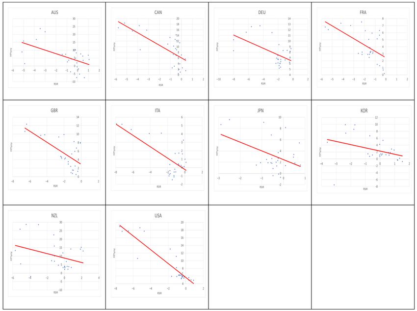
Urban Sci. 2023, 7, 18                                                                                                   6 of 18

                              Similarly, the macroeconomic data series, including the quarterly GDP growth rates,
                         unemployment rates, nominal short- and long-term interest rates, and inflation rates of each
                         country were collected from the OECD (2022a) [36]. These variables were included to test
                         the top three macroeconomic determinants of house prices, viz. the economic factor [21]),
                         the employment factor [57] and the monetary policy factor. Several robustness tests were
                         also conducted by using long-term interest rates and cross-section weights to test their
                         sensitivities to the terms of interest rates and the cross-country heteroscedasticity. Table 1
                         presents the descriptive statistics, and Table 2 reports the stationarities of the variables by
                         using the Levin, Lin and Chu test and the Im, Peasaran and Shin test. They show that all
                         the series are stationary in their first differences.

                         Table 1. Descriptive Statistics of Variables for 2015 Q1–2022 Q3. Sources: OECD (2022a) [36].

                                                                                 Standard
                                  Variable             Country       Mean                        Minimum        Maximum
                                                                                 Deviation
                                                         AUS          0.013         0.025          –0.031          0.025
                                                         CAN          0.020         0.019          –0.032          0.056
                                                         DEU          0.018         0.007           0.008          0.034
                              ∆HPI, House                FRA          0.010         0.006          –0.004          0.022
                               Price Index               GBR          0.014         0.011          –0.003          0.039
                            Quarter-on-Quarter           ITA          0.003         0.009          –0.021          0.019
                                 Change                  JPN          0.008         0.010          –0.007          0.032
                                                         KOR          0.004         0.021          –0.100          0.023
                                                         NZL          0.022         0.026          –0.027          0.081
                                                         USA          0.020         0.015          –0.020          0.049
                                                         AUS         –0.796         1.847          –5.141          1.125
                                                         CAN         –1.152         1.685          –5.755          0.386
                                                         DEU         –2.217         2.095          –7.996          0.097
                                                         FRA         –1.600         1.423          –5.647          0.287
                           RSIR, Real Short-term         GBR         –1.622         1.749          –6.563          0.270
                             Interest Rate (%)           ITA         –1.583         2.071          –7.908          0.294
                                                         JPN         –0.466         0.841          –2.890          0.778
                                                         KOR         –0.121         1.371          –3.607          1.525
                                                         NZL         –0.434         2.447          –5.686          3.392
                                                         USA         –1.514         2.420          –7.523          0.875
                                                         AUS          0.615         1.768           –6.758         3.855
                                                         CAN          0.415         2.716          –10.928         9.018
                                                         DEU          0.291         2.494           –9.481         9.005
                               ∆GDP, Gross               FRA          0.376         4.327          –13.503        18.280
                             Domestic Product            GBR          0.425         5.083          –20.991        16.609
                            Quarter-on-Quarter           ITA          0.277         3.683          –12.101        14.450
                               Change (%)                JPN          0.124         1.946          –7.952         5.575
                                                         KOR          0.635         0.950           –3.027         2.348
                                                         NZL          0.747         3.376          –10.394        13.675
                                                         USA          0.529         2.192           –8.484         7.854
                                                         AUS         5.450          0.809           3.476          7.089
                                                         CAN         6.845          1.553           5.067         12.867
                                                         DEU         3.555          0.465           2.900          4.500
                                                         FRA         8.865          1.027           7.267         10.433
                           UNE, Unemployment             GBR         4.435          0.574           3.600          5.600
                                Rate (%)                 ITA         10.394         1.268           7.933         12.533
                                                         JPN         2.794          0.340           2.300         3.500
                                                         KOR         3.661          0.363           2.733          4.333
                                                         NZL         4.465          0.729           3.200          5.700
                                                         USA         4.938          1.873           3.567         12.967
                                 Period                                        2015 Q1–2022 Q3
                          Number of Observations                      310 Obs (31 periods × 10 countries)
Urban Sci. 2023, 7, 18 7 of 18
Table 2. Unit Root Tests of Variables, 2015 Q1–2022 Q3.
Variable Level First-Difference
Im, Peasaran Im, Peasaran
Levin, Lin & Levin, Lin &
and Shin and Shin
Chu t* Chu t*
W-stat W-stat
log(HPI), log House Price
Index and dlog (HPI),
House Price 6.96 7.92 –1.82 ** –4.40 ***
Quarter-on-Quarter
Change (%)
RSIR, Real Short-term
4.61 1.07 –5.60 *** –7.68 ***
Interest Rate (%)
RLIR, Real Long-term
6.10 6.20 –7.13 *** –6.58 ***
Interest Rate (%)
dlog(GDP), Gross Domestic
Product Quarter-on-Quarter - - –23.74 *** –19.51 ***
Change (%)
UNE, Unemployment Rate
–0.24 –0.63 –13.24 *** –13.03 ***
(%) and d(UNE)
Notes: figures are statistics; ***, ** and * represent p-values ≤ 0.01, 0.05 and 0.10, respectively. The panel unit root
tests used Newey-West automatic bandwidth selection and Quadratic Spectral kernel, with automatic lag length
selection based on SIC: 0 to 5, and automatic selection of maximum lags.
3.2. Research Design
Equation (1) shows the panel regression model used to test the monetary policy
hypothesis.
dlog( HPIi,t ) = β 1 d( RSIRi,t ) + β 2 dlog( GDPi,t ) + β 3 d(UNEi,t ) + αi + γdlog( HPIi,t−1 ) + ε i,t (1)
where the house price index ( HPIi,t ), real short-term interest rate ( RSIRi,t ), gross domestic
product ( GDPi,t ), and unemployment rate (UNEi,t ) of country i at time t are included. αi
controls cross-country fixed effects, and γdlog( HPIi,t−1 ) caters to the autoregressive effect
of house price changes in a one-quarter lag (AR (1)). β 1 , β 2 , β 3 , γ are coefficients to be
estimated. ε i,t is the error term.
A cross-country panel study, however, cannot sort out endogeneity biases. This study
therefore made use of the hikes and falls in the global interest rates during the COVID-19
period as the treatment and the treatment reversal, respectively, of the quasi-experiments
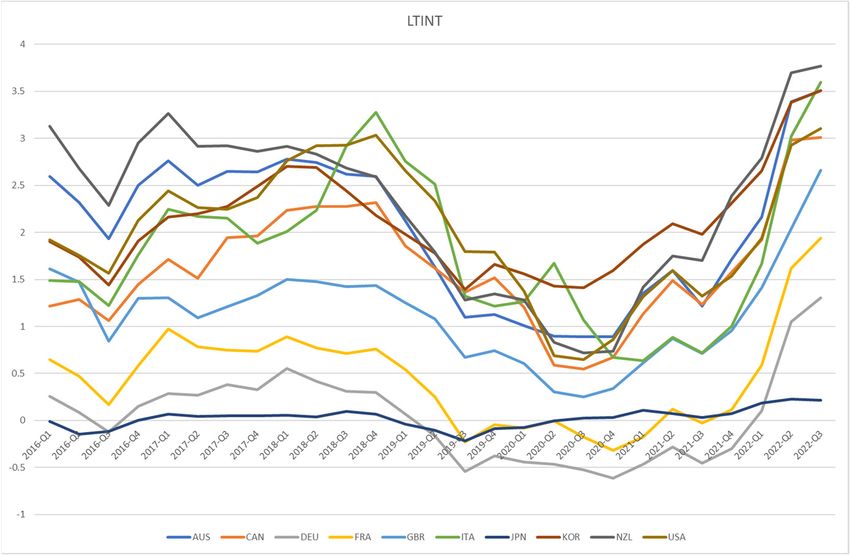
to study the monetary policy hypothesis. As stylized facts, Figure 3 shows the house price
indices of the ten countries from 2015 Q1 to 2022 Q3 (2015 = 100). All showed positive
growth rates in 2020 and 2021, with the peaks of NZL, CAN and the USA, respectively,
ranked as the top three. However, five out of the ten house price indices started to decrease
in 2022. The house price indices of AUS and NZL fell the earliest, with peaks in 2021 Q4,
whereas those of CAN, the USA, and KOR fell later, with peaks in 2022 Q2. The house
prices of the other five countries still showed increases in 2022 Q3, including those of ITA
and JPN.
The pandemic has caused a global recession in 2020 and a rebound in 2021. Figures 4 and 5
show the GDP quarterly growth rates and the unemployment rates from 2015 Q1 to 2022
Q3 for the ten countries.
The quarterly growth rates of the GDPs of many countries were negative in 2020 and
positive in 2021; similarly, unemployment rates were high in 2020, especially in the USA
and CAN, and then became lower since 2021. These could not be the reasons for the house
price rises in 2020–2021 and the falls in 2022. These special scenarios provide a strong test of
the monetary policy hypothesis as other macroeconomic factors, such as GDP growth rates
and unemployment rates, imposed opposite effects against the central banks’ contrarianstudy therefore made use of the hikes and falls in the global interest rates during the
COVID-19 period as the treatment and the treatment reversal, respectively, of the quasi-
experiments to study the monetary policy hypothesis. As stylized facts, Figure 3 shows
the house price indices of the ten countries from 2015 Q1 to 2022 Q3 (2015 = 100). All
showed positive growth rates in 2020 and 2021, with the peaks of NZL, CAN and the USA,
Urban Sci. 2023, 7, 18 8 of 18
respectively, ranked as the top three. However, five out of the ten house price indices
started to decrease in 2022. The house price indices of AUS and NZL fell the earliest, with
peaks in 2021 Q4, whereas those of CAN, the USA, and KOR fell later, with peaks in 2022
efforts
Q2. Thein house
adjusting their
prices of monetary policies
the other five to tackle
countries stillthe recessionary
showed situations
increases in 2020
in 2022 Q3, and
includ-
the inflationary ones in
ing those of ITA and JPN.2022.
Urban Sci. 2023, 7, x FOR PEER REVIEW 9 of 19
monetary policies of central banks [27], there are some contentions that the pandemic also
brought demands for more residential space [58], as well as that the supply chain disrup-
tions during the pandemic could also result in higher construction costs and less housing
supply [59]. Previous single-shock quasi-experiments using COVID-19 did not control
well for the variable of housing supply.
This study exploited two interest rate shocks, as the supply chain disruptions have
not been completely resolved, and the demand for bigger houses is still strong, but house
prices in many countries have started leveling off or even falling down. Yiu (2023) [51]
explicitly controlled for housing supply in a one-country two-shock study and confirmed
the monetary policy hypothesis. This paper further extended to a ten-country two-shock
Figure3.3. House
Figure House price
price indices
indices of
of ten
ten countries
countries from
from 2015
2015 Q1
Q1 to
to 2022
2022 Q3.
Q3. Source:
Source: data
datafrom
from OECD
OECD
model [36].
(2022a) to tackle theAustralia
Legend: insufficient
(AUS), housing
Canada supply
(CAN), contentions.
Germany InFrance
(DEU), other words,
(FRA), by including
Great Britain
(2022a) [36].
the global Legend: Australia (AUS), Canada (CAN), Germany (DEU), France (FRA), Great Britain
(GBR), Italy inflation crisis
(ITA), Japan as aSouth
(JAP), quasi-experiment,
Korea (KOR), New it could
Zealandprovide
(NZL), aand
strong test for
the United the of
States mon-
(GBR), Italy (ITA), Japan (JAP), South Korea (KOR), New Zealand (NZL), and the United States of
etary policy
America (USA). hypothesis, as insufficient housing supply scenarios can only make an under-
America (USA).
estimation of the global interest rate hike effect.
The pandemic has caused a global recession in 2020 and a rebound in 2021. Figures
4 and 5 show the GDP quarterly growth rates and the unemployment rates from 2015 Q1
to 2022 Q3 for the ten countries.
The quarterly growth rates of the GDPs of many countries were negative in 2020 and
positive in 2021; similarly, unemployment rates were high in 2020, especially in the USA
and CAN, and then became lower since 2021. These could not be the reasons for the house
price rises in 2020–2021 and the falls in 2022. These special scenarios provide a strong test
of the monetary policy hypothesis as other macroeconomic factors, such as GDP growth
rates and unemployment rates, imposed opposite effects against the central banks’ con-
trarian efforts in adjusting their monetary policies to tackle the recessionary situations in
2020 and the inflationary ones in 2022.
The use of two interest rate shocks of opposite directions within a short time is one
of the major novelties of this study. This is because, even though the rebounds in house
prices globally after the outbreak of COVID-19 in 2020 were found empirically to be
caused by the synchronized reductions in interest rates and the more accommodative
Figure4.4.Quarter-on-quarter
Figure Quarter-on-quarterpercentage
percentagechange
change inin the
the GDPs
GDPs of of
tenten countries
countries from
from 2015
2015 Q1Q1 to 2022
to 2022
Q3. Source: data from OECD (2022a) [36]. Legend: Australia (AUS), Canada (CAN), Germany
Q3. Source: data from OECD (2022a) [36]. Legend: Australia (AUS), Canada (CAN), Germany (DEU),
(DEU), France (FRA), Great Britain (GBR), Italy (ITA), Japan (JAP), South Korea (KOR), New Zea-
France (FRA), Great Britain (GBR), Italy (ITA), Japan (JAP), South Korea (KOR), New Zealand (NZL),
land (NZL), and the United States of America (USA).
and the United States of America (USA).Urban
UrbanSci.
Sci. 2023,
2023, 7, 18
x FOR PEER REVIEW 1018of 19
9 of
Figure5.5.Unemployment
Figure Unemploymentrates ratesofoftenten countries
countries from
from 20152015 Q12022
Q1 to to 2022
Q3. Q3. Source:
Source: datadata
fromfrom
OECD OECD
(2022a)[36].
(2022a) [36].Legend:
Legend:Australia
Australia(AUS),
(AUS), Canada
Canada (CAN),
(CAN), Germany
Germany (DEU),
(DEU), France
France (FRA),
(FRA), Great
Great Britain
Britain
(GBR),Italy
(GBR), Italy(ITA),
(ITA),Japan
Japan(JAP),
(JAP), South
South Korea
Korea (KOR),
(KOR), New
New Zealand
Zealand (NZL),
(NZL), andand
the the United
United States
States of of
America (USA).
America (USA).
Theuse
The concerted efforts rate
of two interest of central
shocksbankers in cutting
of opposite interest
directions within rates in early
a short 2020
time is oneand
raising
of ratesnovelties
the major in early 2022 triggered
of this study. Thistwoissynchronized
because, evenglobal
though shocks for short-term
the rebounds in house inter-
prices globally
est rates. after thethe
However, outbreak of COVID-19
long-term in 2020
interest rate is were found empirically
considered more relevantto betocaused
housing
by the synchronized
markets reductions
as it is market determinedin interest rates and the
and represents moreexpectations.
market accommodative monetary
As shown in Fig-
policies of central banks [27], there are some contentions that the pandemic also
ures 1 and 6, the patterns of short-term and long-term interest rates of the ten countries in brought
demands
this periodforwere
more highly
residential spacewith
similar [58],some
as well as that the supply
differences. chain
First, they alldisruptions
showed induring
general a
the pandemic could also result in higher construction costs and
U-shaped (a downward and then an upward) trend . The almost-zero long-term less housing supply [59].
rates of
Previous single-shock quasi-experiments using COVID-19 did not control
JPN were also similar to the short-term rate, but the long-term rates of ITA were positive well for the
variable of housing supply.
and much higher than its short-term rate. The long-term rates of Germany and France also
This study exploited two interest rate shocks, as the supply chain disruptions have
dived into the negative zone during the COVID-19 period.
not been completely resolved, and the demand for bigger houses is still strong, but house
prices in many countries have started leveling off or even falling down. Yiu (2023) [51]
explicitly controlled for housing supply in a one-country two-shock study and confirmed
the monetary policy hypothesis. This paper further extended to a ten-country two-shock
model to tackle the insufficient housing supply contentions. In other words, by including
the global inflation crisis as a quasi-experiment, it could provide a strong test for the
monetary policy hypothesis, as insufficient housing supply scenarios can only make an
underestimation of the global interest rate hike effect.
The concerted efforts of central bankers in cutting interest rates in early 2020 and
raising rates in early 2022 triggered two synchronized global shocks for short-term interest
rates. However, the long-term interest rate is considered more relevant to housing markets
as it is market determined and represents market expectations. As shown in Figures 1 and 6,
the patterns of short-term and long-term interest rates of the ten countries in this period
were highly similar with some differences. First, they all showed in general a U-shaped
(a downward and then an upward) trend. The almost-zero long-term rates of JPN were
also similar to the short-term rate, but the long-term rates of ITA were positive and much
higher than its short-term rate. The long-term rates of Germany and France also dived into
the negative zone during the COVID-19 period.
Figure 6. Long term interest rates before and after the outbreak of COVID-19. Source: data from
OECD (2022a) [36]. Legend: Australia (AUS), Canada (CAN), Germany (DEU), France (FRA), Greatmarkets as it is market determined and represents market expectations. As shown in Fig-
ures 1 and 6, the patterns of short-term and long-term interest rates of the ten countries in
this period were highly similar with some differences. First, they all showed in general a
U-shaped (a downward and then an upward) trend . The almost-zero long-term rates of
JPN were also similar to the short-term rate, but the long-term rates of ITA were positive
Urban Sci. 2023, 7, 18 10 of 18
and much higher than its short-term rate. The long-term rates of Germany and France also
dived into the negative zone during the COVID-19 period.
Figure6.6.Long
Figure Longterm
terminterest
interestrates
rates before
before and
and after
after thethe outbreak
outbreak of COVID-19.
of COVID-19. Source:
Source: datadata
fromfrom
OECD (2022a) [36]. Legend: Australia (AUS), Canada (CAN), Germany (DEU), France (FRA),
OECD (2022a) [36]. Legend: Australia (AUS), Canada (CAN), Germany (DEU), France (FRA), Great Great
Britain (GBR), Italy (ITA), Japan (JAP), South Korea (KOR), New Zealand (NZL), and the United
States of America (USA).
4. Results
Figure 7 shows the correlation scatterplots of each country from 2016 Q1 to 2022 Q3. A
universal negative association between house price changes and real interest rates is found
by the best fit lines for all ten countries. However, a scatterplot does not control for other
factors, such as the economic growth and unemployment effects. The results of the panel
regression analysis are reported below.
The empirical results of the ten-country panel regression model, with cross-country
fixed effect and AR (1), are reported in Table 3. In the ten-country full period panel model
(Model 1), the sign and magnitude of the quarterly change in the real short-term interest
rate d(RSIR) coefficient are negative at about −0.58% and statistically significant at the 1%
level, ceteris paribus. Excluding the two control group countries (ITA and JPN) in Model
2, the eight-country panel model shows a stronger negative effect (–0.62%) of real interest
rate change on house price change. The control group (Model 3) shows a weak negative
but insignificant effect of real interest rate change on house price change. These results
reinforce the casual observations that countries with stronger changes in real interest rate
impose stronger effects on house price changes.
When dividing the period in two, with only the first global interest rate shock period
from 2015 Q1 to 2021 Q3 in Model 4 and both the first and the second shock period from
2018 Q4 to 2022 Q3 in Model 5, the d(RSIR) effect in Model 4 is less negative at about –0.32%
and that in Model 5 was the most negative at about –0.71%. Both are significant at the
1% level, ceteris paribus. The magnitude indicates a stronger impact of monetary policy
change on housing market during the whole pandemic period in Model 5. Further taking
both cross-country and period fixed effects, the results in Table 4 also confirm the negative
impact of real interest rate on house price change at a similar magnitude.
In this special period, there were two global and synchronized interest rate interven-
tions imposed by central bankers in the wake of the outbreak of the COVID-19 pandemic
in 2020 and the emergence of the global inflation since 2022. The synchronized responses
of house prices in correspond to the changes in real interest rates in the countries, therefore,
implying a causation relationship of real interest rate change on house price change on the
basis of temporal precedence and counterfactual dependence.Figure 7 shows the correlation scatterplots of each country from 2016 Q1 to 2022 Q
A universal negative association between house price changes and real interest rates
found by the best fit lines for all ten countries. However, a scatterplot does not control
Urban Sci. 2023, 7, 18 other factors, such as the economic growth and unemployment effects. The results
11 of 18 of t
panel regression analysis are reported below.
Figure 7. Scatterplots
Figure ofofhouse
7. Scatterplots house prices year-on-year
prices year-on-year changes
changes (HPIyoy)
(HPIyoy) and realand real short-term
short-term interest inter
rates (RSIRs), for for
rates (RSIRs), 2015 Q1–2022
2015 Q1–2022 Q3, inten
Q3, in tencountries.
countries. Source:
Source: dataOECD
data from from (2022a)
OECD[36].
(2022a) [36]. Lege
Legend:
Australia
Australia (AUS),
(AUS), Canada(CAN),
Canada (CAN), Germany
Germany(DEU),(DEU), France (FRA),
France Great Britain
(FRA), Great (GBR),
BritainItaly (ITA),Italy (IT
(GBR),
JapanJapan
(JAP),(JAP), South
South Korea(KOR),
Korea (KOR), New
NewZealand
Zealand(NZL),
(NZL),and the
andUnited States ofStates
the United America
of(USA).
America (USA).
Table 3. Results of the ten-country panel regression models on house price change and real short-term
The empirical
interest results of the
rates, with cross-country fixedten-country panel regression model, with cross-coun
effect and AR (1).
fixed effect and AR (1), are reported in Table 3. In the ten-country full period panel mod
Model 1—Ten- Model 2—Eight- Model 3—Two- Model 4—Ten- Model 5—Ten-
Dependent (Model
Country 1), the sign
Panel, andPanel,
Country magnitude of the
Country quarterly
Panel, change
Country Panel,in theCountry
real short-term
Panel, inter
Variables
rate d(RSIR) coefficient are negative at about −0.58% and statistically significant at the
2015 Q1–2022 Q3 2015 Q1–2022 Q3 2015 Q1–2022 Q3 2015 Q1–2021 Q3 2018 Q4–2022 Q3
Constant level,(6.42)
0.0112 ceteris
*** paribus. Excluding
0.0124 (5.45) *** the two
0.0057 (3.01)control
*** group countries
0.0142 (7.12) *** (ITA and JPN)
0.0127 (4.41) *** in Mo
d(RSIR) −0.0058 (−4.77) *** −0.0062 (−4.53) *** −0.0012 (−0.56) −0.0032 (−3.23) *** −0.0071 (−4.17) ***
2, the eight-country panel model shows a stronger negative effect (–0.62%) of real inter
dlog(GDP) −0.0002 (−0.79) 0.0001 (0.41) −0.0009 (−2.54) ** −0.0001 (−0.85) −0.0002 (−0.84)
d(UNE) rate change
−0.0016 (−1.98) ** on − house
0.0011 (price
−1.26) change. −0.065The control−group
(−1.63) 0.0017 (−(Model
3.02) *** 3)−shows
0.0016 (−a1.61)
weak negat
AR (1) 0.5573
but insignificant effect of real interest rate change on house price change.***These resu
(9.16) *** 0.5963 (8.88) *** 0.4157 (2.96) *** 0.6878 (13.61) *** 0.5498 (6.20)
Dep. Var. reinforce the casual observations that countries dlog(HPI)
with stronger changes in real interest r
Fixed Effect Cross-country
No. of impose
10 countriesstronger
× 8effects
countrieson× house2price changes.
countries × 10 countries × 10 countries ×
Observations When dividing
29 quarters the period in 29
29 quarters two, with only the
quarters first global interest
25 quarters rate shock peri
16 quarters
Adj. R-sq 0.43 0.43
from 2015 Q1 to 2021 Q3 in Model 4 0.32 and both the first 0.59
and the second0.39 shock period fro
parentheses are t-statistics; *** and ** represent p-values ≤ 0.01 and 0.05, respectively.
2018 Figures
Q4 toin2022 Q3 in Model 5, the d(RSIR) effect in Model 4 is less negative at abou
0.32% and that in Model 5 was the most negative at about –0.71%. Both are significant
The economic growth factor shows a negative and insignificant association with house
price change in most of the models. The unemployment rate factor shows a negative associationUrban Sci. 2023, 7, 18 12 of 18
with house price change and is only statistically significant in Model 1 and Model 4. In addition,
all models show a strong autoregressive pattern in house price change.
Intuitively, the results showed that housing prices are shaped by monetary policy. An
expansionary or contractionary monetary policy triggered a rise or fall of house prices
in the world, respectively, after controlling for the economic, unemployment, individual
country, and period fixed effects.
Table 4. Results of the ten-country panel regression models on house price change and real short-term
interest rates, with both cross-country and period fixed effects.
Model 1a—Ten- Model 2a—Eight- Model 3a—Two- Model 4a—Ten- Model 5a—Ten-
Dependent
Country Panel, Country Panel, Country Panel, Country Panel, Country Panel,
Variables
2015 Q1–2022 Q3 2015 Q1–2022 Q3 2015 Q1–2022 Q3 2015 Q1–2021 Q3 2018 Q4–2022 Q3
Constant 0.0121 (13.74) *** 0.0143 (13.33) *** 0.0066 (7.83) *** 0.0130 (18.55) *** 0.0135 (9.05) ***
d(RSIR) −0.0053 (−3.03) *** −0.0037 (−1.66) * 0.0036 (1.82) * −0.0015 (−0.95) −0.0067 (−2.69) ***
dlog(GDP) −0.0002 (−0.37) −0.0001 (−0.06) −0.0029 (−3.99) *** −0.0004 (−0.99) −0.0002 (−0.27)
d(UNE) −0.0017 (−1.52) −0.0011 (−0.89) −0.0002 (−0.06) −0.0015 (−1.69) * −0.0019 (−1.34)
Dep. Var. dlog(HPI)
Fixed Effects Cross-country and Period
No. of 10 countries × 8 countries × 2 countries × 10 countries × 10 countries ×
Observations 30 quarters 30 quarters 30 quarters 26 quarters 16 quarters
Adj. R-sq 0.40 0.42 0.71 0.53 0.39
Figures in parentheses are t-statistics; *** and * represent p-values ≤ 0.01 and 0.10, respectively.
Robustness Tests
As a robustness test for the sensitivity of the terms of interest rates, Table 5 shows the
empirical results of using real long-term interest rates in the regression models. The results
are highly similar to the ones using real short-term interest rates above. For example, in
the ten-country panel models (Model 6 and Model 10), the effects of d(RLIR) are negative
at about –0.29% and –0.34% on house price changes respectively. The signs, magnitudes
and significances of the effects of the GDP growth factor and unemployment rate factor are
almost the same as above. The results indicate that the market long-term interest rates are
strongly shaped by the central banks’ short-term interest rates [60]. Using either short-term
or long-term interest rates does not greatly affect much the results of the effect of real
interest rate change on house price change.
Table 5. Results of the ten-country panel regression models on house price change and real long-term
interest rates, with cross-country fixed effect and AR (1).
Model 6—Ten- Model 7—Eight- Model 8—Two- Model 9—Ten- Model 10—Ten-
Dependent
Country Panel, Country Panel, Country Panel, Country Panel, Country Panel,
Variables
2015 Q1–2022 Q3 2015 Q1–2022 Q3 2015 Q1–2022 Q3 2015 Q1–2021 Q3 2018 Q4–2022 Q3
Constant 0.0114 (5.72) *** 0.0123 (4.67) *** 0.0058 (2.99) *** 0.0142 (6.91) *** 0.0131 (3.77) ***
d(RLIR) −0.0029 (−2.23) ** −0.0034 (−2.26) ** –0.0006 (–0.30) −0.0027 (−2.71) *** −0.0034 (−1.82) *
dlog(GDP) –0.0001 (–0.37) 0.0002 (0.87) –0.0009 (–2.51) ** –0.0001 (–0.81) –0.0001 (–0.40)
d(UNE) –0.0016 (–1.95) * –0.0010 (–1.14) –0.0066 (–1.66) –0.0016 (–2.73) *** –0.0017 (–1.58)
AR (1) 0.5969 (9.95) *** 0.6345 (9.55) *** 0.4386 (3.18) *** 0.6957 (13.99) *** 0.6043 (6.91) ***
Dep. Var. dlog(HPI)
Fixed Effect Cross-country
No. of 10 countries × 8 countries × 2 countries × 10 countries × 10 countries ×
Observations 29 quarters 29 quarters 29 quarters 25 quarters 16 quarters
Adj. R-sq 0.39 0.39 0.32 0.59 0.34
Figures in parentheses are t-statistics; ***, ** and * represent p-values ≤ 0.01, 0.05 and 0.10, respectively.
Another robustness test for the sensitivity of the cross-section heteroscedasticity is
conducted by re-estimating the long-term interest rate models with panel EGLS cross-Urban Sci. 2023, 7, 18 13 of 18
section weights and White cross-section standard errors and covariance. Table 6 shows the
empirical results, which improve the significance and adjusted R-squared values of the
results in Table 5.
Table 6. Results of the ten-country panel regression models on house price change and real long-term
interest rates, with panel EGLS (cross-section weights and White cross-section standard errors and
covariance.
Model 6a—Ten- Model 7a—Eight- Model 8a—Two- Model 9a—Ten- Model 10a—Ten-
Dependent
Country Panel, Country Panel, Country Panel, Country Panel, Country Panel,
Variables
2015 Q1–2022Q3 2015 Q1–2022 Q3 2015 Q1–2022 Q3 2015 Q1–2021 Q3 2018 Q4–2022 Q3
Constant 0.0117 (8.68) *** 0.0127 (7.80) *** 0.0058 (3.18) *** 0.0150 (5.22) *** 0.0136 (7.05) ***
d(RLIR) −0.0025 (−2.88) *** −0.0029 (−3.13) *** −0.0013 (−0.79) −0.0018 (−2.26) ** −0.0030 (−2.53) **
dlog(GDP) −0.0002 (−1.31) −0.00003 (−0.15) −0.0011 (−5.40) *** −0.0002 (−1.02) −0.0002 (−2.10) **
d(UNE) −0.0024 (−3.63) *** −0.0018 (−3.13) *** −0.0052 (−1.74) * −0.0017 (−4.97) *** −0.0028 (−3.51) ***
AR (1) 0.5548 (7.86) *** 0.5963 (8.37) *** 0.4407 (2.98) *** 0.7515 (11.16) *** 0.5042 (4.86) ***
Dep. Var. dlog(HPI)
Fixed Effect Cross-country
Homoscedasticity Panel EGLS (cross-country weights) and White cross-section standard errors & covariance
No. of 10 countries × 8 countries × 2 countries × 10 countries × 10 countries ×
Observations 29 quarters 29 quarters 29 quarters 25 quarters 16 quarters
Adj. R-sq 0.47 0.47 0.41 0.66 0.39
Figures in parentheses are t-statistics; ***, ** and * represent p-values ≤ 0.01, 0.05 and 0.10, respectively.
The third robustness test is to extend the sampled countries to all the OECD countries
with RIR and HPI data available, to eliminate any sample selection biases, as the treatment
and control groups in the ten-country sample are not randomly assigned. Table 7 shows
that the negative effect of real interest rate changes on house price changes is valid and
has a similar magnitude in the 36-country panel regression model (Model 11). Several
robustness tests are conducted to examine the sensitivity of the level and volatility of real
interest rates. Models 12 and 13 show the results of the countries with high and low RIR,
and Models 14 and 15 show those of volatile and stable RIR. The former is defined as when
the mean of a country’s RIR is higher or lower than the mean of the cross-country means,
whereas the latter is defined as when the standard deviation of a country’s RIR is higher
or lower than the mean of the cross-country standard deviations. All of the results show
the same signs, with similar magnitudes in the coefficients of the real interest rate changes.
They confirm that the monetary policy effect on house prices is valid across all the OECD
countries and is not limited to the ten countries studied above.
Table 7. Robustness tests results of the 36-country panel regression models on house price change
and real long-term interest rates, and sensitivity tests.
Model 12—21- Model 13—15- Model 14—20- Model 15—16-
Model 11—36-
Dependent Country Panel of Country Panel of Country Panel of Country Panel of
Country Panel,
Variables Low RIR, 2015 High RIR, 2015 Stable RIR, 2015 Volatile RIR, 2015
2015 Q1–2022 Q3
Q1–2022 Q3 Q1–2022 Q3 Q1–2022 Q3 Q1–2022 Q3
d(RLIR) −0.0023 (−2.86) *** −0.0021 (−1.94) * −0.0025 (−2.00) ** −0.0020 (−1.65) * −0.0020 (−1.76) *
Dep. Var. dlog(HPI)
Fixed Effect Cross-country and Period
No. of 36 countries × 21 countries × 15 countries × 20 countries × 16 countries ×
Observations 31 quarters 31 quarters 31 quarters 31 quarters 31 quarters
Adj. R-sq 0.36 0.37 0.34 0.34 0.31
Figures in parentheses are t-statistics; ***, ** and * represent p-values ≤ 0.01, 0.05, and 0.10, respectively.Urban Sci. 2023, 7, 18 14 of 18
5. Discussion
Even though housing prices have been escalating to such a level that housing in many
cities is considered unaffordable [61], many people are keen to jump on the bandwagon
by taking a longer mortgage repayment period or borrowing more by paying a mortgage
insurance premium. One of the major reasons why so many people are fond of homeown-
ership is because of the wealth accumulation benefit of housing assets. “Housing is the
principle vehicle of wealth accumulation for the typical household is because it can be
acquired with debt” [13]. According to OECD (2022b) data [62], housing wealth represents
50.4% of household total wealth on average, and mortgage debt accounts for the largest
part (68.6% on average) of total household debt. As a result, housing and monetary policies
have wealth distributional implications.
Thus, it is completely imaginable that, when the central banks reduced interest rates
sharply and relaxed mortgage loan restrictions at the beginning of the pandemic, investors
and home buyers were strongly incentivized to buy houses. On the one hand, lower interest
rates and higher loan-to-value ratios imply that home buyers can pay smaller mortgage
repayment amounts and invest with higher leverage, i.e., a smaller down-payment. On the
other hand, interest rate also determines the market required yield of investments [45], and
a lower yield rate prices property higher, keeping rental income constant.
In contrast, when interest rate is increased, homeowners with outstanding mortgage
loans and new homebuyers have to pay more for their monthly mortgage payments, as the
most common types of mortgage loans in developed countries are either floating rate or
short-term fixed rate. In addition, they also have to bear the risk of having their housing
assets becoming negative equities (market price falls below the outstanding loan amount).
This can incur substantial capital loss if they have to sell the asset, or it may also trigger the
loan-call clause in mortgage contracts where lenders can demand that borrowers repay the
loans immediately.
Nowadays, housing affordability is more commonly measured by the mortgage re-
payment amount to income ratio, as it can accurately estimate the proportion of disposable
income to be consumed and can be benchmarked with the rental payment for a similar
house. However, it depends a lot on monetary policy, including mortgage rate, loan-to-
value ratio, debt-to-income ratio, etc. In some countries, families are encouraged to own
their homes, and favourable mortgage policies, such as negative gearing and higher loan-
to-value ratio for first-time home buyers, etc., are provided. In the past few decades when
interest rates had been relatively low, house prices in many countries escalated rapidly,
investors and homebuyers were attracted to the housing markets. Housing is considered
unaffordable when the house price to income ratio is measured. However, buying homes
can become more attractive and affordable if the mortgage repayment amount to income
ratio is measured. Many low-to-medium-income households may consider it a golden
opportunity to accumulate wealth by acquiring homes with mortgages when borrowing
and repayment are easier. Thus, mortgage loans constitute the single largest debt item of
households over their lifetimes.
When central bankers increase interest rates and tighten mortgage-lending restrictions,
house prices fall but the mortgage repayment amount increases. Is housing more affordable
as the house price to income ratio falls? Interestingly, housing becomes even more unafford-
able than before for home buyers with credit constraints. Even though house prices have
decreased, potential home buyers do not consider housing more affordable even when
their incomes are unchanged, as mortgage loans are more expensive and down-payments
and market risks are much higher.
Contrary to the proposal of the World Economic Forum [12], it can be a myth to
use monetary policy to solve the housing affordability problem. A loosened mortgage
policy seems to enable more people to buy homes with smaller down-payments and lower
mortgage rates, etc., but it causes higher house prices, which can exacerbate the housing
affordability problem. On the contrary, a tightened mortgage policy can bring down houseYou can also read