Atmosphere-ocean-aerosol-chemistry-climate model SOCOLv4.0: description and evaluation - GMD
←
→
Page content transcription
If your browser does not render page correctly, please read the page content below
Geosci. Model Dev., 14, 5525–5560, 2021
https://doi.org/10.5194/gmd-14-5525-2021
© Author(s) 2021. This work is distributed under
the Creative Commons Attribution 4.0 License.

Atmosphere–ocean–aerosol–chemistry–climate model SOCOLv4.0:
description and evaluation
Timofei Sukhodolov1,2,3,4 , Tatiana Egorova1,2 , Andrea Stenke2 , William T. Ball5 , Christina Brodowsky2 ,
Gabriel Chiodo2,6 , Aryeh Feinberg2,7,8 , Marina Friedel2 , Arseniy Karagodin-Doyennel1,2 , Thomas Peter2 ,
Jan Sedlacek1 , Sandro Vattioni2 , and Eugene Rozanov1,2,3
1 Physikalisch-Meteorologisches    Observatorium Davos and World Radiation Center, Davos, Switzerland
2 Institute for Atmospheric and Climate Science, ETH Zurich, Zurich, Switzerland
3 St. Petersburg State University, St. Petersburg, Russia
4 Institute of Meteorology and Climatology, University of Natural Resources and Life Sciences, Vienna, Austria
5 Department of Geoscience and Remote Sensing, Faculty of Civil Engineering and Geosciences,

TU Delft, Delft, the Netherlands
6 Department of Applied Physics and Applied Mathematics, Columbia University, New York, NY, USA
7 Institute of Biogeochemistry and Pollutant Dynamics, ETH Zurich, Zurich, Switzerland
8 Eawag, Swiss Federal Institute of Aquatic Science and Technology, Dübendorf, Switzerland

Correspondence: Timofei Sukhodolov (timofei.sukhodolov@pmodwrc.ch)

Received: 6 February 2021 – Discussion started: 11 March 2021
Revised: 13 July 2021 – Accepted: 27 July 2021 – Published: 8 September 2021

Abstract. This paper features the new atmosphere–ocean–            cent climate and ozone layer trends make SOCOLv4.0 ideal
aerosol–chemistry–climate model, SOlar Climate Ozone               for studies devoted to future ozone evolution and effects of
Links (SOCOL) v4.0, and its validation. The new model              greenhouse gases and ozone-destroying substances, as well
was built by interactively coupling the Max Planck Insti-          as the evaluation of potential solar geoengineering measures
tute Earth System Model version 1.2 (MPI-ESM1.2) (T63,             through sulfur injections. Potential further model improve-
L47) with the chemistry (99 species) and size-resolving (40        ments could be to increase the vertical resolution, which is
bins) sulfate aerosol microphysics modules from the aerosol–       expected to allow better meridional transport in the strato-
chemistry–climate model, SOCOL-AERv2. We evaluate its              sphere, as well as to update the photolysis calculation mod-
performance against reanalysis products and observations of        ule and budget of mesospheric odd nitrogen. In summary, this
atmospheric circulation, temperature, and trace gas distribu-      paper demonstrates that SOCOLv4.0 is well suited for appli-
tion, with a focus on stratospheric processes. We show that        cations related to the stratospheric ozone and sulfate aerosol
SOCOLv4.0 captures the low- and midlatitude stratospheric          evolution, including its participation in ongoing and future
ozone well in terms of the climatological state, variability       model intercomparison projects.
and evolution. The model provides an accurate representation
of climate change, showing a global surface warming trend
consistent with observations as well as realistic cooling in the
stratosphere caused by greenhouse gas emissions, although,         1   Introduction
as in previous model versions, a too-fast residual circulation
and exaggerated mixing in the surf zone are still present. The     Global modeling of the atmosphere and its interaction with
stratospheric sulfur budget for moderate volcanic activity is      oceans, cryosphere, biosphere, and land surface dates back
well represented by the model, albeit with slightly underes-       several decades (e.g., Manabe and Bryan, 1969). The nu-
timated aerosol lifetime after major eruptions. The presence       merical approximation of each of these Earth system com-
of the interactive ocean and a successful representation of re-    ponents is a complex task by itself, and therefore their de-
                                                                   velopment often began and continued independently from

Published by Copernicus Publications on behalf of the European Geosciences Union.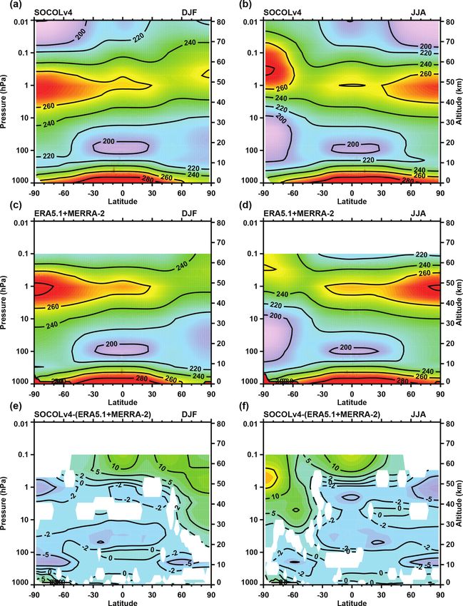
5526                             T. Sukhodolov et al.: Atmosphere–ocean–aerosol–chemistry–climate model SOCOLv4.0

each other, with simplified descriptions of missing, but im-     recovery) are able to significantly affect the tropospheric cli-
portant, processes included in the form of boundary condi-       mate (Previdi and Polvani, 2014; Brönnimann et al., 2017),
tions. With the rapid development of computational facil-        and even the climate response to global warming might be bi-
ities and methods, the models grew in their complexity in        ased if ozone feedbacks are not taken into account (Nowack
terms of the number of processes described and the quality       et al., 2015).
of their description. Motivated primarily through the context       The main driving issue in middle atmosphere chemistry
of climate change research, scientific advances in global nu-    research was the discovery of the ozone hole in the 1980s
merical modeling have shown that, even though stand-alone        (Farman et al., 1985). The ozone layer plays an important
approximations are still sufficient for some specific mod-       role in shielding the biosphere from dangerous solar ultravi-
eling tasks, the interaction of Earth system components is       olet radiation and the risk of related increasing cases of skin
required for reasonable model performance in many cases.         cancer and other diseases induced progress in atmospheric
These advances can be tracked in the history of the Cli-         ozone science that led to strong limitations on the production
mate Model Intercomparison Project (CMIP) requirements           of halogen-containing ozone-depleting substances (hODS)
for models in its different phases (https://www.wcrp-climate.    in 1987 through the Montreal Protocol and its Amendments
org/wgcm-cmip, last access: 2 September 2021). Due to the        (MPA). Since then, observations and models have demon-
importance of the dynamical links between the troposphere        strated the positive role of these restrictive measures (e.g.,
and the stratosphere (Kidston et al., 2015), many climate        Velders et al., 2007; Egorova et al., 2013) and some signs
groups have also extended their state-of-the-art models verti-   of the ozone recovery have already been observed (Chipper-
cally into the mesosphere (e.g., Manzini et al., 2006) or even   field et al., 2017). However, the expected recovery in the
the thermosphere (e.g., Whole Atmosphere Community Cli-          lower stratosphere has been questioned, based on the up-
mate Model (WACCM), Marsh et al., 2013; and the Hamburg          dated observations (Ball et al., 2018, 2019). This issue is
Model of the Neutral and Ionized Atmosphere (HAMMO-              one of many requiring further investigation and deeper un-
NIA), Schmidt et al., 2006). For example, variations in the      derstanding. Other issues and research fields include the ap-
stratospheric polar night jet can induce significant changes     pearance of an unprecedentedly large ozone hole over the
in surface weather on timescales ranging from daily to long-     Northern Hemisphere in spring 2020 (Witze, 2020; Man-
term climate effects (e.g., Gerber et al., 2012, and refer-      ney et al., 2020); the formation of a large and deep Antarc-
ences therein). Variability of this dynamical coupling can       tic ozone hole in autumn 2020 (NASA Ozone Watch, https:
be induced by the Earth system itself, i.e., responding to       //ozonewatch.gsfc.nasa.gov/, last access: 2 September 2021);
ocean temperature changes and vertically propagating wave-       continuous unexpected chlorofluorocarbon (CFC)-11 emis-
forcing from the troposphere, or by external factors such as     sions (Fleming et al., 2020); a potential decline of the solar
volcanic eruptions, variations in the solar UV irradiance, and   activity (Arsenovic et al., 2018); the potential stratospheric
greenhouse gas changes (Kidston et al., 2015).                   injection of sulfur-containing species for solar geoengineer-
   Middle atmosphere studies are closely linked to the rep-      ing purposes (Tilmes et al., 2009; Vattioni et al., 2019); and
resentation of atmospheric chemistry since the ozone layer       a potential impact of increasing trends of iodine in the strato-
primarily determines the temperature structure of the strato-    sphere (Koenig et al., 2020). These examples underline that
sphere through the absorption of solar ultraviolet (UV) irra-    our understanding of atmospheric ozone specifically, and at-
diance. This has an influence on the general circulation of      mospheric chemistry in general, is far from being fully re-
the stratosphere and subsequently also on the tropospheric       solved and inspires further model developments and studies
climate. Stratospheric ozone itself is influenced by many fac-   of the ozone layer evolution, in the present and future.
tors, such as the heterogeneous chemistry intensification af-       The need to represent the large number of processes in-
ter volcanic eruptions (e.g., Revell et al., 2016) or the ac-    volved in the state evolution of the ozone layer led to the
celeration of ozone destruction cycles after energetic par-      development of atmospheric chemistry models ranging from
ticle precipitation events (Rozanov et al., 2012; Mironova       simple box models to chemistry-transport models and finally
et al., 2015). Moreover, it is also largely affected by cli-     to chemistry–climate models that include at least interactive
mate change, via radiatively induced changes in upper strato-    chemistry and atmospheric dynamics but may include ocean
spheric chemistry, as well as changes in the Brewer–Dobson       dynamics, aerosol microphysics, and other components
circulation (BDC, Chiodo et al., 2018). Changes in ozone         (https://www.sparc-climate.org/activities/ccm-initiative, last
can also in turn affect the BDC (e.g., Polvani et al., 2019).    access: 2 September 2021). The chemistry–climate model
Therefore, changes in stratospheric ozone and dynamics feed      SOCOL (SOlar Climate Ozone Links) was initially devel-
back on each other. Ozone-circulation feedbacks have been        oped for studies related to the ozone layer (Egorova et al.,
assessed in several studies, showing their importance for        2005). Through its versions (from v1 to v3), it was used
stratosphere–troposphere coupling in mid-winter (Haase and       with prescribed sea surface temperature and sea ice cover-
Matthes, 2019; Oehrlein et al., 2020) and polar stratospheric    age fields, advancing over time in terms of model numerics,
temperature variability in springtime (Rieder et al., 2019).     stratospheric chemistry, and transport representation. Since
Long-term stratospheric ozone variations (e.g., depletion and    the publication of the base version SOCOLv3 (Stenke et al.,

Geosci. Model Dev., 14, 5525–5560, 2021                                          https://doi.org/10.5194/gmd-14-5525-2021
T. Sukhodolov et al.: Atmosphere–ocean–aerosol–chemistry–climate model SOCOLv4.0                                            5527

2013), the atmospheric-chemistry part has undergone many
further improvements, such as an addition of the volatile or-
ganic compound (VOC) chemistry, an interactive lightning
NOx parameterization, corrections in schemes for solar heat-
ing rates and photolysis rates, parameterization of energetic
particles, and interactive deposition schemes. The base ver-
sion of Stenke et al. (2013), however, further branched into
two significant subversions: SOCOL-MPIOM with interac-
tive ocean (Muthers et al., 2014) and SOCOL-AER with in-
teractive aerosol microphysics (Sheng et al., 2015), each of
them receiving further, independent, upgrades (Arsenovic et
al., 2018; Feinberg et al., 2019), and several smaller variants,
such as an improved tropospheric ozone budget (Revell et
al., 2015, Revell et al., 2018), detailed methane sources and      Figure 1. Components and information flow in the atmosphere–
sinks (Feinberg et al., 2018), and atmospheric selenium cy-        ocean–aerosol–chemistry–climate model SOCOLv4. Green boxes
cling (Feinberg et al., 2020).                                     symbolize prescribed boundary conditions.
   The natural next step was to combine the multiple im-
provements and model versions into a single fourth version
of the SOCOL model by coupling these updated modules               mained unchanged from its predecessor, ECHAM5. Trans-
onto an upgraded atmospheric model, since it also under-           port is calculated every dynamical time step (15 min). The
went many improvements in recent years. As a basis for             dry and wet deposition of gases and aerosols is also based
this, we used the Max Planck Institute Earth System Model          on the ECHAM6 parameters such as near-surface turbulence
(MPI-ESM1.2), so that the chemistry (MEZON) and aerosol            and precipitation. In the following, we discuss each of these
(AER) models are attached to the atmosphere (ECHAM6.3),            main components separately and describe the latest changes.
ocean (MPIOM1.6.3), land surface (JSBACH3.2), ocean                   SOCOLv4 is based on the low-resolution (LR) configura-
biogeochemistry (HAMOCC6) model coupled through the                tion of the MPI-ESM model. This configuration corresponds
OASIS3-MCT coupler. In this paper, we describe the new             to a spectral truncation at T63 providing an approximate
atmosphere–ocean–aerosol–chemistry–climate SOCOLv4.0               horizontal grid spacing of 1.9◦ × 1.9◦ . The vertical resolu-
model and its components in detail (Sect. 2) and validate          tion of the atmosphere is set to 47 levels from the surface
its performance against available observations and reanalysis      to 0.01 hPa, using a hybrid sigma–pressure coordinate sys-
products. The main motivation is to provide a solid reference      tem. Although other higher horizontal and vertical resolu-
of model performance for future improvements and applica-          tions of MPI-ESM are also tuned and available for use, we
tions, including model intercomparison projects (MIPs). The        chose the LR configuration since it is the most used, better
validation is split into two main parts: atmospheric dynamics      tuned (Mauritsen et al., 2019), and better suited for long-term
(Sect. 3.2) and atmospheric chemistry with the primary focus       climate simulations in terms of required computational re-
on stratospheric ozone (Sect. 3.3).                                sources and storage. It must be noted that we did not change
                                                                   anything in the tuning of the MPI-ESM1.2 LR model version
                                                                   described in Mauritsen et al. (2019). All our changes refer to
2   Model description                                              the coupled chemistry and sulfate aerosols modules. Mostly
                                                                   due to the large number of new tracers introduced, SOCOLv4
SOCOLv4.0 (SOCOLv4 hereafter) consists of the Earth sys-           is about 2.6 times slower than MPI-ESM, 30 % of which is
tem model MPI-ESM1.2 (Mauritsen et al., 2019), the chem-           from AER.
istry model MEZON (Egorova et al., 2003), and the sulfate
aerosol microphysical model AER (Weisenstein et al., 1997),        2.1   MPI-ESM1.2 Earth system model
with all these parts being interactively coupled to each other,
as schematically presented in Fig. 1. In simple terms, chem-       The Earth system model MPI-ESM1.2 (Mauritsen et al.,
istry and aerosol microphysics rely on atmospheric temper-         2019) is a further development of its predecessor, MPI-
ature, winds, and relative humidity and in turn influence the      ESM (Giorgetta et al., 2013). The main components of MPI-
atmosphere and ocean through the short- and longwave radi-         ESM are highlighted by the blue boxes in Fig. 1. The ocean
ation schemes, while aerosol microphysics depend on sulfur         dynamical model, MPIOM1.6.3, transports tracers of the
chemistry and provide the aerosol surface area density and         ocean biogeochemistry model, HAMOCC6. The atmosphere
number density necessary for heterogeneous chemistry cal-          model, ECHAM6.3, is directly coupled to the land model,
culations. Transport of individual gases and aerosols is per-      JSBACH3.2, through surface exchange of mass, momentum,
formed by the flux-form semi-Lagrangian scheme of Lin and          and heat. These two major model blocks are then coupled via
Rood (1996) in the dynamical core of ECHAM6 that has re-           the OASIS3-MCT coupler (Craig et al., 2017). The coupler

https://doi.org/10.5194/gmd-14-5525-2021                                             Geosci. Model Dev., 14, 5525–5560, 2021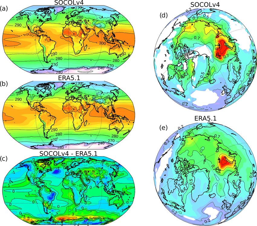
5528                              T. Sukhodolov et al.: Atmosphere–ocean–aerosol–chemistry–climate model SOCOLv4.0

aggregates, interpolates, and exchanges fluxes and state vari-     2.1.2   Marine biogeochemistry model HAMMOC
ables once a day between ECHAM6-JSBACH and MPIOM-
HAMOCC. Here, we only describe the latest states of the            Ocean biogeochemistry in MPI-ESM is represented by the
MPI-ESM components that are used in SOCOLv4 and do                 Hamburg Ocean Carbon Cycle (HAMOCC) model (Ilyina
not focus on the differences between MPI-ESM versions,             et al., 2013; Paulsen et al., 2017). It simulates the oceanic
as this is already discussed in greater detail by Mauritsen        cycles of carbon and other biogeochemical elements such as
et al. (2019). Hereafter we refer to MPI-ESM1.2 as MPI-            nutrients (phosphate, nitrate, and iron), oxygen, silicate, phy-
ESM, and ignore version numberings for other components,           toplankton, zooplankton, and detritus. HAMOCC includes
unless otherwise stated. In terms of differences to the earlier    biogeochemical processes in the water column, the sediment,
versions, we only focus on those between the atmospheric           and at the air–sea interface. Biogeochemical tracers in the
part of the latest version, ECHAM6, and the atmospheric            water column are fully advected, mixed, and diffused by the
part used in SOCOLv3, ECHAM5.4, as changes between                 flow field of MPIOM. In total, the model has 17 state vari-
versions contribute the differences between the chemical re-       ables calculated prognostically in the water column and 12
sponse of SOCOLv4 and all subversions of SOCOLv3.                  state variables in the sediment. Nitrogen-fixing cyanobacte-
                                                                   ria was added to the model as an additional prognostic phy-
2.1.1   Ocean model MPIOM                                          toplankton class by Paulsen et al. (2017).

The oceanic part, MPIOM, is formulated on an Arakawa-              2.1.3   Land surface model JSBACH
C grid in the horizontal and on z levels in the vertical
direction and solves the primitive equations with the hy-          The Jena Scheme for Biosphere-Atmosphere Coupling in
drostatic and Boussinesq approximations (Jungclaus et al.,         Hamburg (JSBACH) is the land component of MPI-ESM1.2.
2006„ 2013). Subgrid-scale parameterizations include lateral       It provides the lower boundary conditions for the atmosphere
mixing on isopycnals and tracer transports by unresolved ed-       over land and describes the dynamics of the land biogeo-
dies. Vertical mixing is represented as a combination of the       chemistry in interaction with global climate. JSBACH treats
Richardson-number-dependent scheme and the wind-driven             processes like soil hydrology (five-layer scheme of Hage-
turbulent mixing in the mixed layer (for details, see Jung-        mann and Stacke, 2015), soil and litter decomposition, land
claus et al., 2013). The horizontal grid is consistent with the    use change (tiling approach with 12 plant functional types
MPI-ESM LR configuration, which implies a bipolar grid             and two types of bare surface), fires, and a nitrogen cy-
(GR1.5) featuring one grid pole under Greenland and one un-        cle (Goll et al., 2017). Note that soil and marine chemical
der Antarctica. The resolutions are then regionally enhanced       schemes are not yet combined with the atmospheric chem-
in the deep water formation regions and the overflows across       istry scheme in the current model version.
the Greenland–Scotland Ridge so that the grid varies be-
tween 22 and 350 km. In the vertical, 40 levels are unevenly       2.1.4   ECHAM6
placed in the water column, with the first 20 levels distributed
over the top 700 m. The bottom topography is represented by        ECHAM6 is an atmospheric general circulation model
a partial-step formulation (Wolff et al., 1997).                   (GCM) that describes the large-scale circulation and its cou-
   The sea ice model combines the codes of MPIOM and               pling to diabatic processes, both of which are ultimately
ECHAM. In ECHAM, a simplified thermodynamic sea ice                driven by radiative forcing. It consists of a dry spectral-
model is incorporated to provide at each atmospheric time          transform dynamical core, a transport model, and a suite of
step a physically consistent surface temperature in ice-           physical parameterizations for the representation of diabatic
covered regions. This part also contains a melt-pond scheme,       processes. The prognostic variables are temperature, vortic-
which divides the surface of the sea ice into snow, bare           ity, divergence, logarithm of surface pressure, and humid-
ice, and melt pond with individual albedos (Pedersen et al.,       ity, as well as cloud ice and water. Tracer transport and di-
2009). The atmospheric part of the sea ice model then inte-        abatic processes (also referred to as “model physics”) are
grates all surface fluxes into ice and provides this informa-      calculated on a Gaussian transform grid. The adiabatic core
tion to the oceanic part of the code, which uses it to calcu-      of ECHAM6 consists of a mixed finite-difference/spectral
late the sea ice surface energy balance and related changes        discretization of the primitive equation that is identical to
in ice thickness. The calculations of sea ice concentration        that employed in ECHAM5 (Stevens et al., 2013). All ma-
and thickness are based on the Semtner (1976) formula-             jor changes relative to ECHAM5 are therefore related to
tion and tuned in MPI-ESM to produce the annual aver-              the model physics. These changes include an improved rep-
age pre-industrial Arctic sea ice volume of roughly 20 000–        resentation of radiative transfer in the shortwave (or solar)
25 000 km3 (see Mauritsen et al., 2019). Sea ice dynam-            part of the spectrum; a completely new description of tro-
ics is calculated following a viscoplastic approach of Hi-         pospheric aerosol; an improved representation of surface
bler (1979).                                                       albedo, including the treatment of melt ponds on sea ice (see
                                                                   Sect. 2.1.1); and an improved representation of the middle at-

Geosci. Model Dev., 14, 5525–5560, 2021                                            https://doi.org/10.5194/gmd-14-5525-2021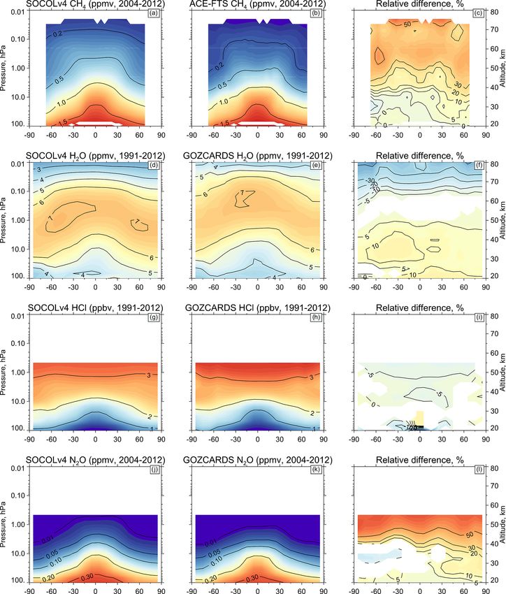
T. Sukhodolov et al.: Atmosphere–ocean–aerosol–chemistry–climate model SOCOLv4.0                                             5529

mosphere through the gravity wave forcing. In addition, mi-      cal depth, asymmetry factor and single scattering albedo as
nor changes have been made in the representation of convec-      a function of geographical position, height above ground
tive processes. Several coding errors in model physics were      level, time, and wavelength. The evolution and distribution
also corrected in the latest version (see details in Mauritsen   of anthropogenic aerosol is approximated with mathemati-
et al., 2019).                                                   cal functions, while the natural aerosol is prescribed climato-
   Transport of species is performed with the flux-form semi-    logically based on Kinne et al. (2013). MACv2-SP also pre-
Lagrangian scheme of Lin and Rood (1996). Though this            scribes aerosol–cloud interactions in the form of a Twomey
scheme is mass conservative by design, its application on the    effect (Twomey, 1977), thus allowing the increase in the
sigma–pressure coordinate system can cause a violation of        cloud droplet number concentration and associated reduction
the mass conservation especially in the case of large spatial    in droplet size under constant liquid water path.
gradients (Jöckel et al., 2001; Stenke et al., 2013). Turbu-
lent mixing adopts an eddy diffusivity and viscosity approach    2.2   Atmospheric chemistry model MEZON
following Brinkop and Roeckner (1995). Moist convection
is parameterized according to Tiedtke (1989), with exten-        The atmospheric chemistry part of the new model is a
sions by Nordeng (1994) and Möbis and Stevens (2012).            modified version of the chemistry-transport model MEZON
Stratiform clouds are computed diagnostically based on a         (Model for Evaluation of oZONe trends; Rozanov et al.,
relative humidity threshold (Sundqvist et al., 1989). As in      2001; Egorova et al., 2003; Schraner et al., 2008). The last
ECHAM5, gravity wave drag (GWD) is calculated using a            base state of this code is described in detail by Stenke et
subgrid orography scheme (Lott, 1999). The propagation and       al. (2013). It underwent major upgrades for participation in
dissipation of the waves follow the formulation of Palmer et     the Chemistry Climate Model Initiative phase 1 (CCMI) pre-
al. (1986) and Miller et al. (1989). Non-orographic GWD          sented in Revell et al. (2015). Further upgrades were made
parameterizations are based on a wave-spectrum approach          in Revell et al. (2018) and Feinberg et al. (2019). Below, we
(Hines, 1997a, b). However, some parameters of both oro-         summarize the current state of MEZON, while the history of
graphic and non-orographic gravity wave schemes have been        main updates that are now included in SOCOLv4 is schemat-
adjusted for use in ECHAM6 during the tuning process of          ically illustrated in Fig. 2. In this paper, the direct comparison
MPI-ESM (see Mauritsen et al., 2019). Both longwave and          with SOCOLv4 is made only for the CCMI version (Revell
shortwave radiative-transfer calculations are now described      et al., 2015) in Sect. 3.2.2 and 3.2.4, since it was the most
by the PSrad scheme (Pincus and Stevens, 2013), which            widely used one in publications.
is based on the k-correlated method of the Rapid Radia-             MEZON and ECHAM6 are interactively coupled by the
tive Transfer Model for GCMs (RRTM-G) (Iacono et al.,            three-dimensional fields of temperature and wind, and by the
2008). Additional extra-heating parameterization in the Hart-    radiative forcing induced by water vapor, ozone, methane,
ley, Huggins, and Schumann–Runge bands and the Lyman-            nitrous oxide, and CFCs. The chemistry scheme is called
α line is now applied for better representation of the so-       every 2 h. The chemical solver is based on the implicit it-
lar cycle in the mesosphere and stratosphere (Sukhodolov         erative Newton–Raphson scheme (Ozolin, 1992; Stott and
et al., 2014). The optical properties for radiation are up-      Harwood, 1993). The model includes 99 chemical species of
dated every 2 h. In contrast to the base model version, which    the oxygen, hydrogen, nitrogen, carbon, chlorine, bromine,
applies climatological fields for this purpose, the radiation    and sulfur groups, which are determined by 216 gas-phase
calculation of SOCOLv4 uses the prognostic tracer concen-        reactions, 72 photolysis reactions, and 16 heterogeneous
trations of sulfate aerosol and all radiatively active species   reactions in/on aqueous sulfuric acid aerosols, as well as
(e.g., ozone and methane) except CO2 . Concentrations for        three types of polar stratospheric clouds (PSCs): supercooled
CH4 , N2 O, and CFCs are prescribed only at the lowermost        ternary solution (STS) droplets, water ice, and nitric acid tri-
model level, while CO2 is prescribed for the entire atmo-        hydrate (NAT). Chemical reaction rate coefficients and ab-
sphere. Note that for photolysis rates calculations, we use a    sorption cross sections of all reactions follow the recommen-
separate subroutine based on the application of lookup tables    dations from NASA JPL data evaluation no. 18 (Burkholder
(Rozanov et al., 1999). Cloud scattering is parameterized ac-    et al., 2015). Photolysis rates are calculated at every chem-
cording to Mie theory using maximum-random cloud over-           ical time step using a lookup-table approach (Rozanov et
lap and an inhomogeneity parameter to account for three-         al., 1999), including effects of the solar irradiance variabil-
dimensional effects. Surface albedo is parameterized accord-     ity. Based on the stand-alone photolysis codes intercompari-
ing to Brovkin et al. (2013). The radiative properties of tro-   son study (Sukhodolov et al., 2016) and additional sensitiv-
pospheric aerosols are now represented by the Max Planck         ity tests, the photodissociation rates of molecular oxygen and
Institute Aerosol Climatology version 2 simple plume im-         ozone (O(1 D) path) have been supplemented by the correc-
plementation (MACv2-SP) parameterization (Stevens et al.,        tion factors of 1.2 for oxygen in the 10–1 hPa region and 1.5
2017; Fiedler et al., 2017). MACv2-SP is formulated in terms     for ozone below 100 hPa.
of nine spatial plumes associated with different major an-          Dry deposition of species is based on the surface resis-
thropogenic source regions. It prescribes the aerosol opti-      tance approach for the estimation of dry deposition velocities

https://doi.org/10.5194/gmd-14-5525-2021                                            Geosci. Model Dev., 14, 5525–5560, 2021
5530                               T. Sukhodolov et al.: Atmosphere–ocean–aerosol–chemistry–climate model SOCOLv4.0

Figure 2. History of main updates through different versions of SOCOL, which contributed to the version described in this paper. Note that
there were also other minor changes, adjustments, and error corrections.

proposed by Wesely (1989). This scheme takes into account              above. In the troposphere, the heterogeneous hydrolysis of
actual meteorological conditions, different surface types, and         N2 O5 on tropospheric aerosols contributes to the sink of
trace gas properties like solubility and reactivity. Further de-       odd nitrogen. Note that since the MACv2-SP parameteriza-
tails are given by Kerkweg et al. (2006). The wet deposition           tion that is used for radiation does not provide the aerosol
scheme is based on the scavenging scheme SCAV proposed                 mass, for the tropospheric chemistry we use the tropospheric
by Tost et al. (2006). Wet deposition velocities are calculated        aerosol climatology that considers the aerosol properties of
using cloud and precipitation variables from ECHAM6, in-               11 Global Aerosol Data Set (GADS, Koepke et al., 1997)
cluding cloud cover, liquid and ice water contents, precipita-         types as in the previous model version. The reaction proba-
tion fluxes, and the convective upward mass flux. Scavenging           bilities for the different aerosol types are calculated follow-
coefficients of gaseous species depend on their Henry’s law            ing the parametrization by Evans and Jacob (2005).
constants. Upon evaporation of clouds and rainwater, scav-                Parameterizations of the N, NO, and OH production by
enged species are transferred back into the gas phase. An              galactic cosmic rays, solar protons, and energetic electrons
additional sink for HNO3 , in the form of a constant removal           with energies of < 300 keV are introduced as 0.55, 0.7, and
rate of 1×10⁻⁶ s−1 , was introduced in the upper troposphere           up to 2 molecules of N, NO, and OH per ion pair, respectively
(above 300 hPa), compensating the missing uptake of HNO3               (Matthes et al., 2017). The contribution of thermospheric NO
by ice particles (e.g., Voigt et al., 2006).                           from downward intrusions is parameterized as a flux-form
   The parameterization of heterogeneous chemistry in the              upper boundary condition (Funke et al., 2016). The lightning
stratosphere is based on Carslaw et al. (1995). It coincides           source of NOx is parameterized based on the cloud top ap-
with HNO3 uptake by aqueous sulfuric acid aerosols result-             proach by Price and Rind (1992). The tropospheric budget
ing in the formation of STS. The parameterization of the               of CO is supplemented by the Mainz Isoprene Mechanism
liquid-phase reactive uptake coefficients follows Hanson and           (MIM-1, Pöschl et al., 2000) that describes the degradation of
Ravishankara (1994) and Hansen et al. (1996). The PSC                  isoprene, formaldehyde, and acetic acid. Contributions of all
scheme for water ice uses a prescribed particle number den-            other non-methane volatile organic compounds (NMVOCs)
sity of 0.01 cm−3 and assumes that the cloud particles are in          to CO is accounted for via the addition of a certain fraction of
thermodynamic equilibrium with their gaseous environment.              NMVOC emissions to CO. For anthropogenic, biomass burn-
NAT is formed if the partial pressure of HNO3 exceeds its              ing, and biogenic NMVOC emissions the conversion factors
saturation pressure, assuming a mean particle radius of 5 µm           to CO are 1.0, 0.31, and 0.83, respectively (Ehhalt et al.,
for NAT. The particle number densities are limited by an up-           2001).
per boundary of 5 × 10⁻⁴ cm−3 to account for the fact that                Several newly discovered hODS (CFC-112, CFC-112a,
observed NAT clouds are often strongly supersaturated. The             CFC-113a, CFC114a, and HCFC-133a) have been added to
sedimentation of NAT and water ice is based on the Stokes              the model chemistry scheme together with some additional
theory as described in Pruppacher and Klett (1997). Water              chlorine containing very-short-lived substances (VSLSs:
ice and NAT are not explicitly transported but are evaporated          CHCl3 , CH2 Cl2 , C2 Cl4 , C2 HCl3 , C2 H4 Cl2 ) that are not con-
back to water vapor and gaseous HNO3 after each chemi-                 trolled by the MPA. The bromine-containing VSLS forcing is
cal time step, transported in the vapor phase, and then de-            now also transient compared to the previous model versions
pending on the saturation conditions regenerated in the next           and includes CH3 Br, CHBr3 , and CH2 Br2 species. The sul-
time step with the thermodynamic approximation described               fur family is represented by eight gas-phase species: carbonyl

Geosci. Model Dev., 14, 5525–5560, 2021                                                  https://doi.org/10.5194/gmd-14-5525-2021
T. Sukhodolov et al.: Atmosphere–ocean–aerosol–chemistry–climate model SOCOLv4.0                                               5531

sulfide (OCS), CS2 , H2 S, dimethyl sulfide (DMS), methane-        2.4   Model setup and boundary conditions
sulfonic acid (MSA), SO2 , SO3 , and H2 SO4 (Sheng et al.,
2015).                                                             As described above, SOCOLv4 is based on the latest version
                                                                   of MPI-ESM that was also used for the Climate Model In-
2.3   Sulfate aerosol microphysics model AER                       tercomparison Project phase 6 (CMIP6) runs. To test the new
                                                                   coupled model, we initialized all its parts from the MPI-ESM
The sulfate aerosol microphysical scheme AER is based on           restart files (snapshots of the model’s state at a specified time)
the two-dimensional sulfate aerosol model of Weisenstein et        from the end of the year 1949 and then continued the calcu-
al. (1997). It was upgraded and combined with SOCOLv3              lation until the end of 2018. The initialization of chemistry
by Sheng et al. (2015) and later further improved by Fein-         was based on SOCOLv3 runs from Revell et al. (2016). In
berg et al. (2019). Sulfate aerosol particles are resolved in 40   1980, the reference run was split into an ensemble of three
size bins, ranging in dry radius from 0.39 nm to 3.2 µm, cor-      runs by imposing a temporary (1-month long) small pertur-
responding to a range of 2.8–1.6 × 10¹² molecules of H2 SO4        bation in atmospheric CO2 concentrations. For the analysis
per particle (assuming an H2 SO4 density of 1.8 g cm−3 ).          performed here, we skip the first 30 years of simulations and
H2 SO4 molecule number doubles between bins, while the             focus on the 1980–2018 period, which is well covered by ob-
corresponding wet sulfate aerosol radii can be much larger         servations.
depending on local conditions. H2 SO4 weight percent is cal-          Model boundary conditions mostly follow the recommen-
culated online based on actual temperature and relative hu-        dations of CMIP6 provided by the input4MIPs database
midity. The AER scheme includes submodules for the nu-             (https://esgf-node.llnl.gov/search/input4mips/, last access:
cleation (Vehkamäki et al., 2002), composition (Tabazadeh          2 September 2021). All forcings are historical before 2015
et al., 1997), growth, evaporation (Ayers et al., 1980; Kul-       and switched to the SSP2-4.5 scenario for the last 4 years
mala and Laaksonen, 1990), coagulation (Fuchs, 1964; Ja-           until 2018. These include concentrations of greenhouse
cobson and Seinfeld, 2004), and sedimentation of sulfate           gases (Meinhausen et al., 2016), surface anthropogenic and
aerosol (Kasten, 1968; Walcek, 2000). In addition to gas-          biomass-burning emissions of NOx (as well as aircraft emis-
phase H2 SO4 production, the model calculates aqueous ox-          sions), CO, SO2 , and NMVOCs (Hoesly et al., 2018), ion-
idation of S(IV) by ozone (O3 ) and hydrogen peroxide              ization rates by galactic cosmic rays, solar protons, and en-
(H2 O2 ) (Jacob, 1986). The spatial distribution of cloud pH in    ergetic electrons, solar spectral irradiance variations, and the
the aqueous-phase chemistry routine is approximated based          influx of thermospheric NO (Matthes et al., 2017). Biogenic
on Tost et al. (2007). The aqueous production flux of S(VI)        emissions of all NMVOCs use a climatology for the year
is added directly to the scavenged aerosol flux in cloud wa-       2000 based on MEGAN (Model of Emissions of Gases and
ter. Dry and wet deposition of sulfate aerosol are calcu-          Aerosols from Nature; Guenther et al., 2006). For the long-
lated by the similar schemes as for gas-phase species (Tost        and short-lived halogenated source gases (ozone-depleting
et al., 2006; Kerkweg et al., 2006). Dry and wet deposi-           substances (ODSs) and VSLSs) we used the World Meteoro-
tion as well as gravitational velocities of sulfate aerosol are    logical Organization (WMO) Ozone Assessment 2018 base-
calculated through radius-dependent parameterizations. Dur-        line mixing ratio scenario, which is a combined atmospheric
ing cloud evaporation, evaporating scavenged sulfate aerosol       observation record up to the year 2017 (Engel et al., 2018).
mass is transferred to the largest aerosol size bin. Transport     For some ODSs, we also used the input4MIPs database.
of aerosols in each bin is also performed in the same way as       Agricultural land-use changes are based on the Land Use
transport of gases with a time step of 15 min. The microphys-      Harmonization project data (LUHv2h, Hurtt et al., 2011).
ical module is called every 2 h with 20 subtime steps yielding        Continuous degassing emissions of SO2 are prescribed ac-
an aerosol microphysical time step of 6 min.                       cording to volcano locations (Andres and Kasgnoc, 1998;
   The influence of the aerosol on radiation fluxes at all         Dentener et al., 2006). To represent eruptive emissions, we
wavelengths (14-band shortwave and 16-band longwave) is            applied a satellite-derived dataset from Carn et al. (2016).
taken into account. Extinction coefficients, single-scattering     Since the emission profiles are unknown in this database,
albedo, and asymmetry factors required by the radiation            they are emitted into the upper third of the total plume height.
codes are treated following a lookup-table approach with pre-      Air–sea DMS fluxes are calculated online through a wind-
calculated aerosol physical properties using Mie theory for        driven parametrization (Nightingale et al., 2000) and clima-
actual H2 SO4 weight percent and temperature using refrac-         tological gridded sea surface DMS concentrations (Lana et
tion indices from Biermann et al. (2000). The aerosol surface      al., 2011). 1 Tg S yr−1 of CS2 is emitted between the lati-
area density and composition are used to calculate heteroge-       tudes of 52◦ S and 52◦ N based on Weisenstein et al. (1997).
neous reaction rates in a chemical module. Note that AER           The surface mixing ratios of H2 S and OCS are prescribed as
aerosols in the model impact chemistry and radiation only in       30 pptv (Weisenstein et al., 1997) and 510 pptv (Timmreck et
the stratosphere. In the troposphere, we use MACv2-SP for          al., 2018), respectively.
radiation and GADS for N2 O5 hydrolysis (see Sect. 2.1.4 and          Since the model vertical resolution is insufficient for a
2.2).                                                              reasonable self-generation of the quasi-biennial oscillation

https://doi.org/10.5194/gmd-14-5525-2021                                              Geosci. Model Dev., 14, 5525–5560, 2021
5532                             T. Sukhodolov et al.: Atmosphere–ocean–aerosol–chemistry–climate model SOCOLv4.0

(QBO), we nudge it to the observed equatorial wind profiles.      (Fig. 3a, b), the Arctic sea ice extension anomaly (Fig. 3c),
The nudging is applied between 20◦ N and 20◦ S from 90 hPa        as well as the El Niño–Southern Oscillation (ENSO) Niño3.4
up to 3 hPa. Within the QBO core domain (10◦ N–10◦ S, 50–         statistics (Fig. 4a, b) for the historical period 1980 to 2018.
8 hPa), the relaxation time is uniformly set to 7 d; outside      Anomalies were calculated as a deviation from the mean over
of this region, the damping depends on latitude and altitude      the 1980–2018 period. Figure 5a, c also show the global
(Giorgetta, 1996).                                                mean 2 m temperature and its anomaly simulated with the
   Tropospheric aerosols are represented by two separate          SOCOLv4 and various reanalysis data. The model reveals a
datasets for radiation and chemistry. For radiation, to be con-   warming trend similar to observations, whereas the ensemble
sistent with the base model and CMIP6 recommendations,            mean curve shows less interannual variability, as expected
we used the MACv2-SP approach (Stevens et al., 2017),             (Fig. 3a). As can be seen from the figure, the reanalysis data
which however provides only optical parameters of aerosols.       slightly disagree in terms of the absolute level and the model
Surface area densities required for the N2 O5 hydrolysis are      data are within this spread. Modeled global mean surface
based on the tropospheric aerosol climatology of 11 aerosol       air temperature is somewhat warmer than the ERA5.1 and
types from GADS (Koepke et al., 1997), as in SOCOLv3.             MERRA-2 data but colder than the BEST data. Tempera-
                                                                  ture anomalies (Fig. 3b) agree very well with observational
                                                                  composites. The annual Arctic sea ice extent anomalies are
3     SOCOLv4 evaluation                                          also accurately reproduced by SOCOLv4 in line with obser-
                                                                  vations, showing a pronounced decline with time because of
3.1     Atmospheric dynamics                                      global warming and fluctuations of magnitudes to observa-
                                                                  tions (Fig. 3c). According to Ding et al. (2019), the spread
3.1.1    Reference data for evaluation
                                                                  in sea ice extent between the ensemble members can be at-
We validate the simulated climate variables from SOCOLv4          tributed to internal variability driven by fluctuations in Arc-
against observations. For this purpose, we use reanalysis data    tic pressure expressed as high pressure enhancing the sea ice
because they incorporate various observations combined in         loss and low pressure restraining it. Based on the analysis
one dataset using comprehensive techniques that allow gaps        of Fig. 3, we conclude that the model response to historical
in space and time to be estimated. It should be noted that        radiative forcing is sufficiently close to observations, which
the combination of different data can lead to some errors in      proves suitability of the model for studies of past and future
the reanalysis data, both in trends and variability, that have    climate changes.
a purely methodological nature, like those due to changes in         ENSO is known as the largest mode of sea surface tem-
the observation systems or aging of instruments as well as        perature anomalies with irregular period of ∼ 2–7 years,
the details of underlying models used for assimilation. In-       which influences atmospheric circulation globally in the tro-
tercomparison of different reanalysis products by Long et         posphere (e.g., Bulgin et al., 2020) as well as in the middle
al. (2017) showed that reanalyses agree in the lower–middle       atmosphere (Domeisen et al., 2019). It is tracked as a vari-
stratosphere but deviate more from each other in the up-          ability of the sea surface temperature in the so-called Niño3.4
per stratosphere and lower mesosphere because of the de-          region (5◦ N–5◦ S, 120–170◦ W). These temperature anoma-
creased availability of direct observations and thus the in-      lies are usually in the range of ±3 K with positive fluctua-
creased dependence on the assimilating model details, like        tions being associated with El Niño events and negative with
the model top and vertical resolution. This should be con-        La Niña events. There were several El Niño events observed
sidered when making conclusions about deviations between          with positive deviations stronger than +1.5 K during the con-
model results and reanalysis. To validate the thermodynam-        sidered decades, with the strongest being those in 1982/1983,
ical structure of the modeled atmosphere, we use the recent       1997/1998, and 2015/2016. To verify the model performance
ERA5.1 reanalysis dataset (Simmons et al., 2020; Hersbach         in this context, we analyzed the fast Fourier transform (FFT)
et al. 2020) from ECMWF (European Centre for Medium-              and the probability density function (PDF) (Fig. 4a and b, re-
Range Weather Forecasts) and MERRA-2 (Modern-Era Ret-             spectively) of the modeled and ERA5.1 Niño3.4 indices. The
rospective Analysis for Research and Applications version 2,      analysis indicates that SOCOLv4 has realistic ENSO in terms
Gelaro et al., 2017). For surface air temperature, we addition-   of amplitude and periodicity; however, the 40-year period
ally use the BEST data (the Berkeley Earth Surface Temper-        is rather short for a robust estimation of ENSO frequencies,
atures, Cowtan et al., 2015), which are a merged land–ocean       which is illustrated as a pronounced variability among the en-
dataset.                                                          semble members. The common bias shared by all members
                                                                  is that ENSO events in the model mostly last longer than in
3.1.2    Temperature and winds                                    observations. This is expressed as the power spectrum shift
                                                                  to shorter frequencies and a flattened PDF. It must be noted
To assess the ability of SOCOLv4 to reproduce the cli-            that this is a known feature of our underlying model, MPI-
mate and its response to historical forcing, we show variabil-    ESM, and our FFT results are very similar to those shown by
ity in annual mean surface air temperature and its anomaly        Müller et al. (2018) in their Fig. 13, where they analyzed a

Geosci. Model Dev., 14, 5525–5560, 2021                                           https://doi.org/10.5194/gmd-14-5525-2021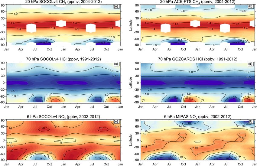
T. Sukhodolov et al.: Atmosphere–ocean–aerosol–chemistry–climate model SOCOLv4.0                                                5533

                                                                       Figure 4. (a) The 1980–2018 Niño3.4 power spectra
                                                                       (◦ C/cycles month−1 ) calculated from the ERA5 data (orange)
                                                                       as well as from the three SOCOLv4 ensemble members (black).
                                                                       Dashed lines are the 95 % significance levels based on an auto-
                                                                       regressive AR(1) process fitting. (b) Histogram of Niño3.4
                                                                       temperature anomalies.
Figure 3. Global and annual mean 2 m temperature (a) and its
anomalies relative to 1980–2018 mean (b) and Arctic sea ice ex-
tent annual anomaly (c) in comparison to reanalysis data. The thick    ulated with SOCOLv4 and derived from the ERA5.1 reanal-
black line represents simulated mean of the three-member SO-           ysis, as well as their difference. ERA5.1 data have been inter-
COLv4 ensemble, thin black lines are individual ensembles mem-         polated to the model grid. SOCOLv4 properly reproduces the
bers, the red line indicates ERA5.1 reanalysis, the green line indi-   observed geographical pattern of the surface air temperature
cates MERRA-2 reanalysis, and the blue line indicates BEST re-
                                                                       with cold high-latitude areas in both hemispheres and warm
analysis.
                                                                       tropics and subtropics. However, there are some regional dis-
                                                                       crepancies between the model and the reanalysis data. The
                                                                       model surface air temperature is generally slightly (∼ 0.2 K)
140-year period. The spatial pattern of ENSO in the model              warmer than in ERA5.1, which is also seen from the global
is reasonable but also has some biases related to the asym-            means (Fig. 3a), but there are also several spots with cold bi-
metry between El Niño and La Niña events (for details see              ases. In the tropical area, the discrepancies are within ±1 K,
Tian et al., 2019). This drawback could be minimized by in-            except in the eastern part of South America over the Brazil-
creasing coupling frequency between ocean and atmosphere               ian Highlands, where negative bias reaches −5 K, and over
from daily to hourly. However, this change also increases the          the Tibetan Plateau and mainland southeast Asia, with up to
computational demands to levels, which are less suitable for           −3 K bias. In the northern middle latitudes, we obtain neg-
long-term climate calculations. Therefore, the LR version of           ative discrepancies of about −5 K over the Rocky Moun-
MPI-ESM which we used for SOCOLv4 was tuned with a                     tains and the North Atlantic Ocean. The most pronounced
daily coupling (Mauritsen et al., 2019).                               biases of ±6 K are located in the Southern Hemisphere over
   The left panel of Fig. 5 shows the geographical distribution        Antarctica. Most of these biases in high-altitude regions are
of the 2 m air temperature climatology for 1980–2018 as sim-           a common feature of all coupled models, which is usually

https://doi.org/10.5194/gmd-14-5525-2021                                                 Geosci. Model Dev., 14, 5525–5560, 2021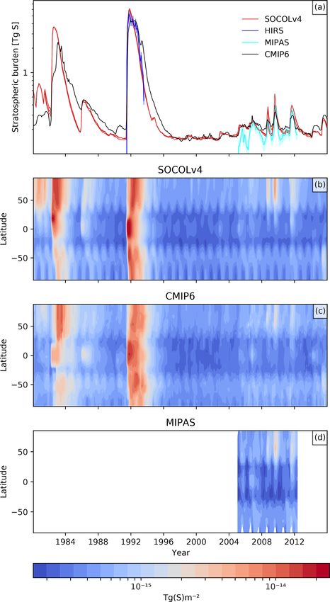
5534 T. Sukhodolov et al.: Atmosphere–ocean–aerosol–chemistry–climate model SOCOLv4.0
westerlies in the midlatitudes to be insufficiently poleward,
which is more pronounced in the Southern Hemisphere and
represented as negative and positive deviations around 60 and
40◦ S, respectively. The differences between the model and
observations increase with altitude. In the stratosphere, the
simulated summertime easterly jets are of similar strength
to those in the observations but have some deviations in
their shapes. The deviations between about 90 and 3 hPa in
the (sub)tropics are related to the hemispherically symmetric
QBO nudging approach, which is applied between 20◦ N and
20◦ S (see Sect. 2.4). The wintertime polar night jets show
larger deviations in both hemispheres. In the Northern Hemi-
sphere, the modeled polar vortex is significantly weaker than
in the observations and is extended equatorward in the lower
mesosphere. The Southern Hemisphere vortex is of similar
strength to that in reanalysis mean data in the stratosphere
and the main model deviations are related to its positioning.
The core of the southern polar jet is shifted to 60◦ and lo-
cated between 10 and 1 hPa, while in the reanalysis data the
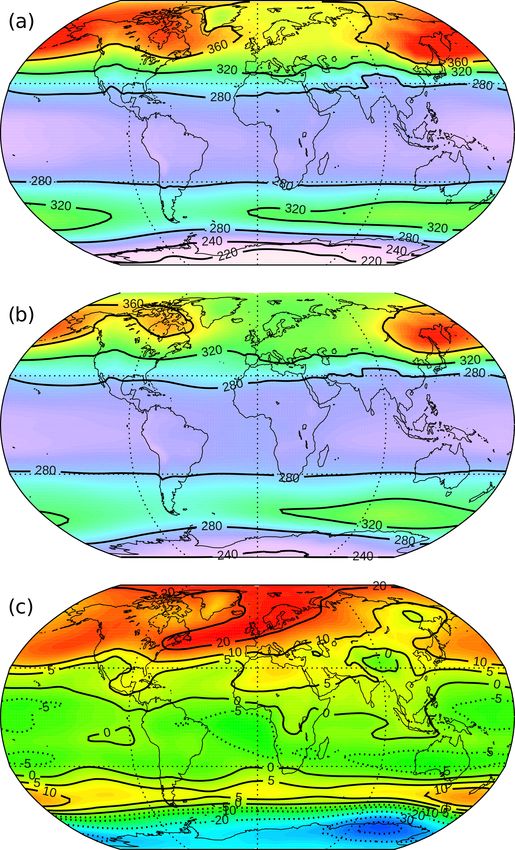
Figure 5. Left panels: global distribution of 2 m surface air temper- vortex core (80 m s−1 isoline) extends higher and shifts to-
ature (K, contours are −5, −3, −1, 0, 1, 3, 5, 7, 9) averaged over
wards 40◦ S. Therefore, the modeled southern polar vortex
the period 1980–2018 simulated by SOCOLv4 (a, ensemble mean),
ERA5.1 reanalysis data (b), and their difference (c, SOCOL4-
area is more isolated in the middle stratosphere. Oppositely,
ERA5.1). Right panels: 2 m surface air temperature trend over the in the lower mesosphere, it is extended equatorwards, simi-
Northern Hemisphere (K/10 years, contours are −0.5, −0.2, 0, 0.2, lar to the northern one. The latter feature might suggest that
0.5, 0.7, 1.0, 1.5) simulated (d) and observed (e) over the Northern there is some overestimation in the gravity wave forcing that
Hemisphere. White spots show where the trend is not statistically is dominant in this region (Plumb, 2002; Butchart, 2014).
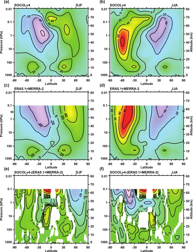
significant at the 95 % level. The zonal mean temperature distribution is generally well
reproduced by the model (Fig. 7), but there are also strong
biases in the middle atmosphere with respect to the obser-
attributed to the simplified model’s topography and uncer- vations that are consistent with the biases in zonal winds.
tainties in the observational data (e.g., Guo et al., 2020). The Namely, the wintertime high-latitude middle and upper
right panel of Fig. 5 shows the 2 m surface air temperature stratosphere and the low mesosphere are warmer by 2–10 K
trends over 1980–2018 over the Northern Hemisphere sim- suggesting weaker vortices and stronger meridional transport
ulated by SOCOLv4 and calculated from ERA5.1 reanaly- and mixing. In the rest of the stratosphere, the difference
sis data. The linear trend and its significance were calcu- is negative (about −2 K). This is consistent with a too-fast
lated using a robust nonparametric Sen–Mann–Kendall test BDC, which would cause increased adiabatic cooling in the
applying 95 % confidence interval. Simulated and observed tropics and in the summertime high latitudes. In the lower-
trends over the Northern Hemisphere show a good spatial most extratropical stratosphere, there are up to −5 K temper-
agreement including the location of the warming maximum ature deviations in both hemispheres, which leads to some
north of Siberia. The maximum simulated trend amounts to downward displacement of the extratropical tropopause. The
1.69 ± 0.16 K, which is only about 0.25 K smaller than the modeled tropospheric temperatures agree very well with ob-
maximum trend of 1.93 K derived from the reanalysis. servations and only show a warm bias over Antarctica.
Zonal mean climatology of zonal winds and temperatures It has to be noted that all of the presented model deviations
for boreal winter and summer as simulated by SOCOLv4 are in thermodynamics are long-term issues of the ECHAM-
presented in comparison to observations (mean data from re- family models and global models in general (Stevens et al.,
analysis ERA5.1 and MERRA-2) in Figs. 6 and 7, respec- 2013; Mauritsen et al., 2019). In Fig. A1, we present the same
tively. Even though the model has an upper limit at 0.01 hPa, differences as in Figs. 6 and 7 but for the pure MPI-ESM
we analyze the results only up to a height of 0.1 hPa, since CMIP6 run. As can be seen from there, SOCOLv4 and MPI-
above ERA5.1 data are not reliable and MERRA-2 data are ESM share the same deviation patterns indicating weaker and
not available. In general, the model reproduces the obser- warmer polar vortices in the stratosphere. Some differences
vations well, but there are deviations which are, however, between SOCOLv4 and MPI-ESM results are mostly related
typical for most coupled models (Bock et al., 2020; Gettel- to the stratospheric ozone distribution at midlatitudes and
man et al., 2019; Matthes et al., 2020). The tropospheric jets, high latitudes, as well as to the distribution of other GHGs
their position, and strength are reasonably reproduced by the except CO2 that are now three-dimensional, and the QBO
model with biases of ±2–5 m s−1 . There is a tendency of the nudging in SOCOLv4 in the tropics. Many of these problem-
Geosci. Model Dev., 14, 5525–5560, 2021 https://doi.org/10.5194/gmd-14-5525-2021T. Sukhodolov et al.: Atmosphere–ocean–aerosol–chemistry–climate model SOCOLv4.0 5535
Figure 6. Zonal mean zonal wind climatology (m s−1 ) for DJF (a, c, e) and JJA (b, d, f) simulated with SOCOLv4 (a, b), mean of ERA5.1
and MERRA-2 reanalysis (c, d), and differences between simulated and reanalysis data (e, f). Contour intervals for the difference are −30,
−20, −10, −5, −2, 2, 5, 10, 20, 30 m s−1 . White areas denote regions where the difference between model and reanalysis data is not
statistically significant at the 95 % confidence level calculated with a Student’s t test.
atic features were shown to be greatly improved using a ver- there is also a limit in model’s scalability defined by hori-
sion of ECHAM with more detailed (95-level) vertical reso- zontal resolution.
lution (Schmidt et al., 2013; Stevens et al., 2013; Mauritsen
et al., 2019; Matthes et al., 2020), especially the strength of 3.2 Atmospheric chemistry and transport
the northern polar vortex and the extratropical lower strato-
spheric cold biases. The increase of the vertical resolution 3.2.1 Reference data for validation
implies, however, a strong increase in computational time,
because of the column physics design. It can be partly com- All datasets that were used for the chemistry validation
pensated by increasing the amount of processing units, but are listed in Table 1. For the comparison of HCl, H2 O,
and N2 O, we used the Global OZone Chemistry And Re-
https://doi.org/10.5194/gmd-14-5525-2021 Geosci. Model Dev., 14, 5525–5560, 20215536 T. Sukhodolov et al.: Atmosphere–ocean–aerosol–chemistry–climate model SOCOLv4.0 Figure 7. Zonal mean temperature climatology for DJF (a, c, e) and JJA (b, d, f) simulated with SOCOLv4 (a, b), mean of ERA5.1 and MERRA-2 reanalysis (c, d), and differences between simulated and reanalysis data (e, f). Contour intervals for the differences are −30, −20, −10, −5, −2, 0, 2, 5, 10, 20, 30, 40 K. White areas denote regions where the difference between model and reanalysis data is not statistically significant at the 95 % confidence level. lated trace gas Data records for the Stratosphere database pared to the BAyeSian Integrated and Consolidated compos- (GOZCARDS, Froidevaux et al., 2015), which is a com- ite ozone (BASIC, Alsing and Ball, 2019), and the CMIP6 posite based on the data from eight satellite instruments. ozone forcing dataset (Checa-Garcia, 2018). The latter is a The Envisat satellite Michelson Interferometer for Passive compilation of CESM1-WACCM and Canadian Middle At- Atmospheric Sounding (MIPAS, Funke et al., 2014) instru- mosphere Model (CMAM) modeling results and is used as ment data were used for NOy , while the SCISAT Atmo- a standard forcing for MPI-ESM. Ozone total column is val- spheric Chemistry Experiment Fourier Transform Spectrom- idated against Multi-Sensor Reanalysis version 2 (MSRv2, eter (ACE-FTS) data climatology is used for NOy and CH4 . Van der A et al., 2015a) and Solar Backscatter Ultravio- Besides GOZCARDS, the ozone mixing ratio is also com- let Spectral Radiometer version 2 (SBUVv8.6) (McPeters Geosci. Model Dev., 14, 5525–5560, 2021 https://doi.org/10.5194/gmd-14-5525-2021
T. Sukhodolov et al.: Atmosphere–ocean–aerosol–chemistry–climate model SOCOLv4.0                                            5537

et al., 2013) composites. Stratospheric aerosol sulfur mass        the model top in the mesosphere is likely related to the treat-
is compared to MIPAS (Günther et al., 2018) and High-              ment of the Lyman-α line photolysis, while the rest is due to
resolution Infrared Radiation Sounder (HIRS) (Baran and            the problems in dynamics. Thus, a too-fast vertical transport
Foot, 1994) observations and a composite recommended by            in the tropics (Fig. 8a–c) would mean that there is less time
CMIP6 (GloSSACv1.1, Thomason et al., 2018).                        for CH4 loss on the way upwards and therefore more CH4
   It has to be noted that observations themselves are not per-    arrives in the mesosphere, which can be partly enhanced by
fect, especially for the shorter-lived species with pronounced     underestimation of CH4 photolysis. Dynamical lifetime got
diurnal cycles, low concentrations, and specific regions like      smaller with respect to chemical lifetime and the tracer be-
high latitudes and the upper troposphere/lower stratosphere        came more vertically mixed. The increased concentration in
(UTLS). Different satellite instruments vary in terms of mea-      the upper stratosphere is then also distributed polewards and
surement method, geographical coverage, spatial and tempo-         downwards in the middle and high latitudes. Difference in
ral sampling and resolution, time period, and retrieval algo-      skewness of the isolines suggests an overestimation of mid-
rithm. All of this has also to be dealt with while constructing    latitude mixing in the upper stratosphere/lower mesosphere,
the observational composites, which imposes further poten-         which is consistent with analysis of winds showing that the
tial uncertainties related to the homogenization methods ap-       vortices are weaker at those altitudes (Fig. 6). Middle and
plied. The SPARC Data Initiative (SPARC, 2017) conducted           lower stratospheric midlatitudes, however, show some hemi-
an overview of the existing trace gases and aerosol measure-       spheric asymmetry with a negative bias of 5 % in the SH
ments and provided a set of useful recommendations con-            and a positive bias of 5 %–10 % in the NH. Figure 9a–b
cerning the related uncertainties that we used in the further      show the CH4 seasonal cycle at 20 hPa and suggests that
sections for our validation.                                       this anomaly is likely related to the deficiencies in horizon-
                                                                   tal mixing. Namely, while the model reproduces very well
3.2.2   Trace gas climatology                                      the tropical values (1.4 ppmv isoline), the midlatitude val-
                                                                   ues (1 ppmv isoline) are excessively shifted poleward in the
In this section, we discuss the SOCOLv4 performance in             NH and slightly equatorward in the SH. This is also gener-
reproducing observed distributions of various trace species.       ally consistent with Fig. 6, which shows at these altitudes a
Figures 8, 11, and 12 show the data from the model and             weaker NH polar vortex and the SH polar vortex that is more
observations and the relative differences between them. Fig-       confined to the pole.
ures 9 and 13 show mean seasonal cycles of several species
that are also compared to observations.                            H2 O

CH4                                                                Water vapor (H2 O) provides a source for hydroxyl radicals
                                                                   (HOx ) in the stratosphere. Hydroxyl catalytic cycles domi-
Methane (CH4 ) is an important source of water vapor (H2 O)        nate the ozone destruction above the stratopause and are also
in the stratosphere. On average, two H2 O molecules are pro-       very important in the lower and middle stratosphere. The two
duced per CH4 molecule oxidized. Methane mixing ratios             main sources of H2 O in the stratosphere are methane oxida-
drop very fast with height due to increasing availability of       tion and the transport from the H2 O-rich troposphere. Trans-
hydroxyl radical (OH), the excited atomic oxygen (O(1 D)),         port from the troposphere is important for the lower strato-
and atomic chlorine (Cl). In the lower mesosphere, photol-         sphere and is highly dependent on the cold point tempera-
ysis by Lyman-α radiation also becomes an important sink           ture at the tropical tropopause and vertical transport in the
for CH4 . Methane is also an important atmospheric tracer for      tropics. As seen from Fig. 8d–f, SOCOLv4 agrees very well
tracking the stratospheric circulation because of its long life-   with observations around the stratopause. In the lower strato-
time. CH4 mixing ratio isolines in Fig. 8b are lifted upward       sphere, the model is 5 %–10 % too moist, which is due to
in the low latitudes by the ascending branch of the BDC and        some overestimation of H2 O at the entry point. In the meso-
are pushed downward in the middle and high latitudes by the        sphere, the model underestimates H2 O by up to 30 % (or
descending branch. Isolines in the midlatitudes are flattened      1 ppmv) around the model top. This partly results from the
as a result of rapid mixing by breaking planetary waves. The       underestimated destruction of methane (about 0.2 ppmv) but
balance between horizontal mixing and the diabatic circula-        mostly comes from the overestimated water vapor photolysis,
tion produces the observed tracer slope and deviations in this     which was also previously reported for SOCOL in the stand-
distribution can hint at potential problems in transport pro-      alone photolysis codes intercomparison study (Sukhodolov
cesses (e.g., Strahan, 2015).                                      et al., 2016; Karagodin-Doyennel et al., 2021). The water va-
   SOCOLv4 nicely reproduces the methane distribution in           por sink (dehydration) by PSCs in the south polar lowermost
the lower stratosphere with only about ±5 % deviations from        stratosphere is well captured by the model.
observations. However, above ∼ 10 hPa, the model deviation            Water vapor is a relatively long-lived species with a highly
gradually increases with height to up to 50 % overestimation       pronounced seasonality in the lower tropical stratosphere.
in the lower mesosphere. The highest overestimation close to       This seasonality is related to tropospheric wave forcing,

https://doi.org/10.5194/gmd-14-5525-2021                                             Geosci. Model Dev., 14, 5525–5560, 2021
You can also read