DNICast Direct Normal Irradiance Nowcasting Methods for Optimized Operation of Concentrating Solar Technologies
←
→
Page content transcription
If your browser does not render page correctly, please read the page content below
DNICast
Direct Normal Irradiance Nowcasting Methods
  for Optimized Operation of Concentrating
             Solar Technologies

                      THEME [ENERGY.2013.2.9.2]
 [Methods for the estimation of the Direct Normal Irradiation (DNI)]
                       Grant agreement no: 608623

       Deliverable Nr.: 2.2                    Deliverable title:
                                          Review of the Potential of
                                      WMO Sand and Dust Storm Warning
                                       Assessment and Analysis System
                                     (SDS-WAS) in Nowcasting/Forecasting
                                        Direct Normal Irradiance (DNI)
   Project coordinator: OME                     WP leader: CyI
   Name of the organization:          Authors: M. Pikridas, M. Vrekoussis,
                                          N. Mihalopoulos, L. Barrie
        Submission date:                         Version nr.:1

Disclaimer: The information and views set out in this report are those of the
author(s) and do not necessarily reflect the official opinion of the European
Union. Neither the European Union institutions and bodies nor any person
acting on their behalf may be held responsible for the use which may be
made of the information contained therein.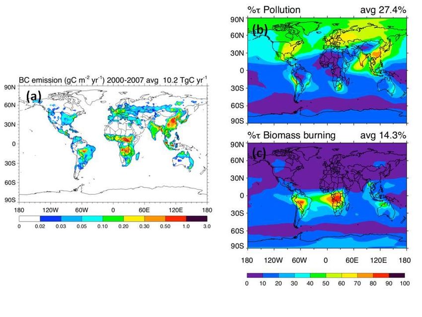
DNICast, Deliverable 2.2

Abstract

The intensity of solar radiation reaching the surface of the Earth is dictated
by clouds, atmospheric suspended particulate matter, commonly known as
aerosols, and to a lesser extent, gases in the atmosphere. Short term
forecasting of solar radiation reaching the Earth’s surface on scales of hours
(nowcasting) is possible using atmospheric numerical models that simulate
not only classic weather but also atmospheric aerosol production, transport,
transformation and removal for a large range of particle sizes (0.1 μm to 10
μm). The focus of this EU project is direct normal irradiance (DNI) at the
Earth’s surface which is the principle variable required to efficiently manage
concentrating solar technologies (CST) engaged in power production.
This report first introduces the reader to fundamentals of atmospheric
science related to processes that control DNI and to the quantitative
forecasting of aerosols and clouds that determine DNI. It then focuses
mainly on aerosols leaving cloud forecasting to another group in this project.
There are many types of aerosols ranging from natural sea salt, sand and
dust, biogenic marine sulphates and terrestrial vegetation organics to
anthropogenic sulphates, nitrates, organics and black carbon. Of these,
sand and dust mobilized by winds from arid regions with little vegetation is
very important for DNI in the North African, Middle East and European
region as well as parts of Asia. In the form of dust storms, it can cause
severe degradation of visibility while suspended in the atmosphere and
fogging/abrasion of mirrors reflecting solar radiation to storage vessels
when deposited on the Earth’s surface.
In recognition of the importance of sand and dust aerosols for DNI, human
health and weather/climate, the World Meteorological Organization (WMO)
has established the Sand and Dust Storm Warning Advisory and Assessment
System (SDS-WAS) to coordinate research and forecasts of sand and dust
properties and their validation with observations for two regions of the
world: (i) North Africa, the Middle East and Europe and (ii) Asia. SDS-WAS
products from many different forecast models in both regions are
accessible on the web1.
A detailed description of SDS-WAS models and their forecast products is
given in this report. Information is provided on how to retrieve forecasts
and analyses from the SDS-WAS website or from the developer of each
model. In several cases, the web pages of individual modeling groups in
SDS-WAS provide cloud cover forecasts that are not accessible in the SDS-

1
    http://www.wmo.int/sdswas

                                                                            ii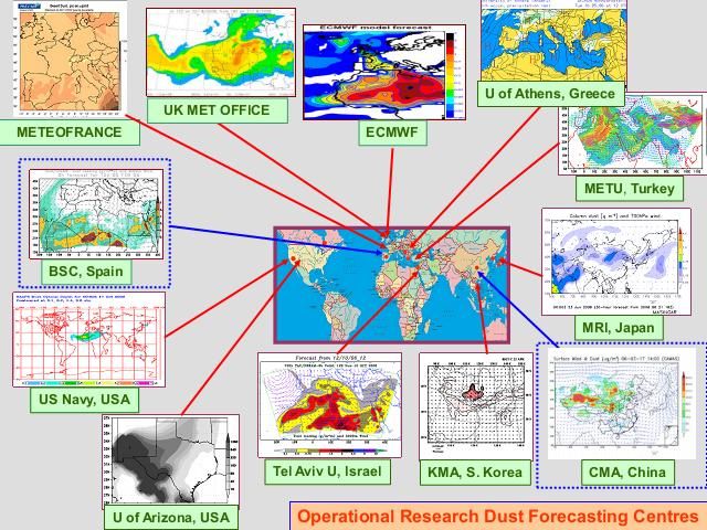
DNICast, Deliverable 2.2

WAS portal. A priori knowledge of aerosol science or of numerical
simulation of weather is not required. Explanation of basic concepts and
terminology is also provided. Also, many models do not stop at sand and
dust aerosols and provide forecasts of all major aerosol types which can
affect DNI. These are introduced as well.

Keywords: SDS-WAS, dust, numerical dust forecast, aerosol properties,
model assessment

                                                                      iii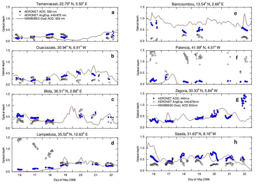
DNICast, Deliverable 2.2

Table of Contents

Abstract .................................................................................................. ii
Table of Contents .................................................................................... 4
List of Figures .......................................................................................... 8
1.     Introduction.................................................................................. 12
2.     Basic Concepts .............................................................................. 14
     2.1      Interactions of Radiation with the Atmosphere ........................... 14
       2.1.1         Beer-Lambert Law ................................................................ 14
       2.1.2         Optical Depth ........................................................................ 16
       2.1.3         Other characteristic optical properties ................................ 19
     2.2      Fundamental Aerosol Properties.................................................. 19
       2.2.1         Particle size is linked with emitting source........................... 19
     2.3      Cloud Condensation Nuclei (CCN) ................................................ 21
     2.4      Aerosol constituents and sources ................................................ 23
       2.4.1         Sea salt .................................................................................. 23
       2.4.2         Mineral Dust ......................................................................... 24
       2.4.3         Sulfate ................................................................................... 27
       2.4.4         Organics ................................................................................ 27
       2.4.5         Black carbon from biomass burning and fossil fuel emissions.
                     28
  2.5  Direct Normal Irradiance (DNI) and Aerosol ................................ 30
3. Simulating the Atmosphere ........................................................... 31
     3.1      Atmospheric Aerosol Modelling ................................................... 32
       3.1.1         Model Types ......................................................................... 32
       3.1.2         Spatial resolution .................................................................. 33
       3.1.3         Parameterization .................................................................. 34
       3.1.4         Simulating the mass size distribution ................................... 34
       3.1.5         Modeled Processes ............................................................... 35
       3.1.6         Emissions .............................................................................. 36

                                                                                                                 4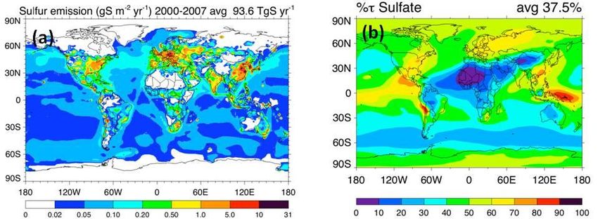
DNICast, Deliverable 2.2

  3.2   WMO - Sand and Dust Storm Warning Advisory and Assessment
  System (SDS-WAS).................................................................................... 36
4. Selected Ground and Satellite Observations .................................. 42
     4.1     Aerosol Robotic NETwork (AERONET) .......................................... 42
     4.2     European Aerosol Research Lidar Network (EARLINET) ............... 43
     4.3     Moderate-resolution Imaging Spectroradiometer (MODIS) ........ 44
5.     Available Dust Simulation Models ................................................. 45
     5.1     MACC-ECMWF .............................................................................. 45
       5.1.1        Model Summary ................................................................... 45
       5.1.2        Model Evaluation.................................................................. 46
       5.1.3        Data Availability .................................................................... 47
     5.2     The DREAM and BSC-DREAM8b ................................................... 48
       5.2.1        Model Summary ................................................................... 48
       5.2.2        Model Evaluation.................................................................. 49
       5.2.3        Data Availability .................................................................... 52
     5.3     TAU/DREAM8b ............................................................................. 52
       5.3.1        Model Summary ................................................................... 52
       5.3.2        Model Evaluation.................................................................. 52
       5.3.3        Data Availability .................................................................... 52
     5.4     TSMS/BSC-DREAM8b .................................................................... 53
       5.4.1        Model Summary ................................................................... 53
       5.4.2        Data Availability .................................................................... 53
     5.5     DREAM8-SEEVCCC ........................................................................ 53
       5.5.1        Model Summary ................................................................... 53
       5.5.2        Data Availability .................................................................... 53
     5.6     NMMB/BSC-Dust .......................................................................... 53
       5.6.1        Model Summary ................................................................... 53
       5.6.2        Model Evaluation.................................................................. 55
       5.6.3        Data Availability .................................................................... 57
     5.7     SKIRON .......................................................................................... 58

                                                                                                               5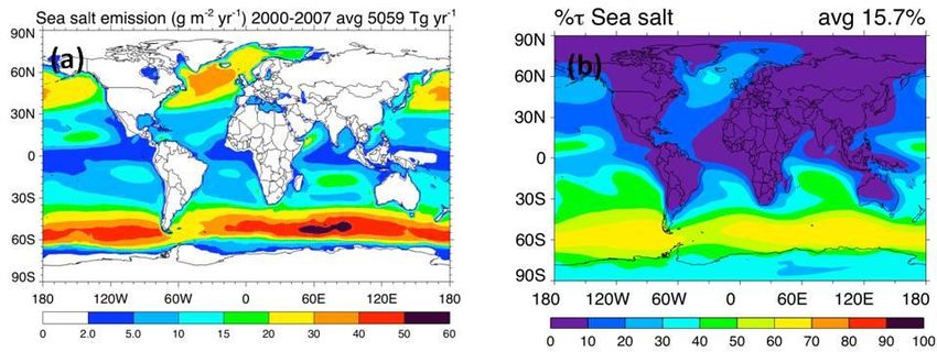
DNICast, Deliverable 2.2

     5.7.1      Model Summary ................................................................... 58
     5.7.2      Model Evaluation.................................................................. 58
     5.7.3      Data Availability .................................................................... 59
  5.8    LMDz-INCA .................................................................................... 59
     5.8.1      Model Summary ................................................................... 59
     5.8.2      Model Evaluation.................................................................. 60
     5.8.3      Data Availability .................................................................... 60
  5.9    CHIMERE ....................................................................................... 61
     5.9.1      Model Summary ................................................................... 61
     5.9.2      Model Evaluation.................................................................. 62
     5.9.3      Data Availability .................................................................... 64
  5.10   NAAPS ........................................................................................... 64
     5.10.1     Model Summary ................................................................... 64
     5.10.2     Model Evaluation.................................................................. 64
     5.10.3     Data Availability .................................................................... 66
  5.11   MetUM ......................................................................................... 66
     5.11.1     Model Summary ................................................................... 66
     5.11.2     Model Evaluation.................................................................. 68
  5.12   NGAC............................................................................................. 70
     5.12.1     Model Summary ................................................................... 70
     5.12.2     Model Evaluation.................................................................. 71
     5.12.3     Data Availability .................................................................... 72
  5.13   GEOS-5 .......................................................................................... 72
     5.13.1     Model Summary ................................................................... 72
     5.13.2     Model Evaluation.................................................................. 73
     5.13.3     Data Availability .................................................................... 74
  5.14   RegCM4 ........................................................................................ 75
     5.14.1     Model Summary ................................................................... 75
     5.14.2     Model Evaluation.................................................................. 75
     5.14.3     Data Availability .................................................................... 76

                                                                                                           6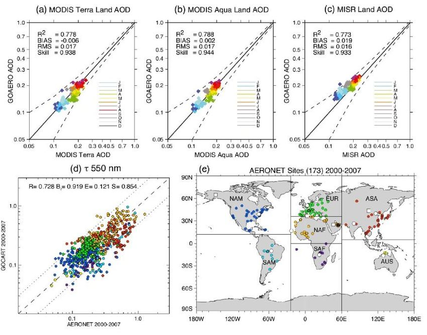
DNICast, Deliverable 2.2

  5.15 Some Tips on the Application of SDS-WAS Aerosol Forecasts for
  Different Regions...................................................................................... 76
6. References .................................................................................... 80
7.     Appendix ...................................................................................... 91
     7.1     Conditioning of SDS-WAS data ..................................................... 91
     7.2     Evaluation Metrics ........................................................................ 92
     7.3     Nomenclature ............................................................................... 94

                                                                                                          7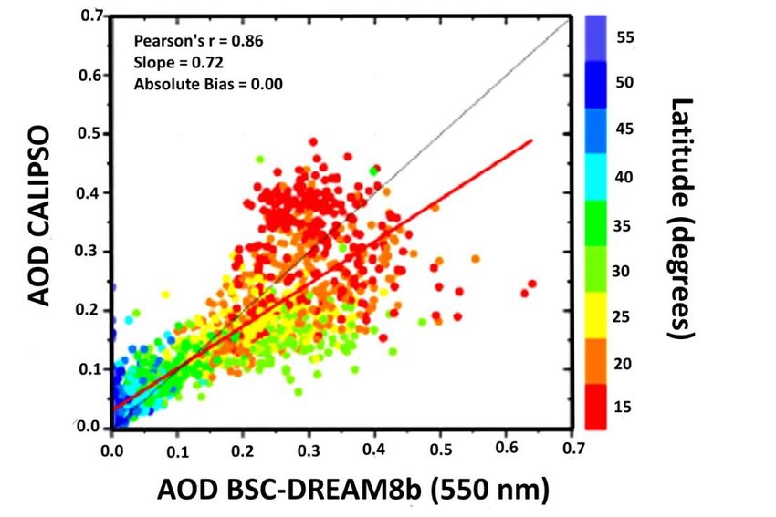
DNICast, Deliverable 2.2

List of Figures

Figure 1: The Earth’s global annual mean energy budget between March
2000 and May 2004 (W m–2). The broad arrows indicate the schematic flow
of energy in proportion to their importance (Trenberth et al., 2009) ......... 13
Figure 2: Solar radiation reaching Earth’s surface. The UV, visible and
infrared parts of the spectrum is depicted. The coloring of the visible part of
the spectrum is also shown. ......................................................................... 15
Figure 3: Dependance of volume-normalized single particle cross section as
a function of particle size for a particle with refractive index equal to
1.5±0.02i (Willeke and Brockmann, 1977). .................................................. 16
Figure 4: A best estimate of the global distribution of annual average
tropospheric aerosol optical depth (AOD 550 nm) compiled by combining
data from six satellites operating for limited periods between 1979 and
2004 (courtesy of S. Kinne MPI, Hamburg, Germany).................................. 18
Figure 5: Typical number and mass distributions of atmospheric particles.
Different modes are depicted in the graph. Because particle diameters span
several orders of magnitude, the x-axis of the graph is in logarithmic scale
(Seinfeld and Pandis, 2006). ......................................................................... 20
Figure 6: Ship tracks (white lines) in marine stratus clouds over the Atlantic
Ocean as viewed from satellite on January 27, 2003. Brittany and the
southwest coast of England can be seen on the upper right side of the
image (Wallace and Hobbs, 2006) ................................................................ 22
Figure 7: Variation of the frequency of supercooled clouds and of clouds
containing snow crystals. Curves (1) and (2) pertain to ordinate on the left;
curves 3 to 6 pertain to ordinate on the right. (1) Peppler (1940) over
Germany, (2) Borovikov et al. (1963) over the ETU, (3) Mossop et al. (1970)
over Tasmania, (4) Morris & Braham (1968) over Minnesota, (5) Isaac &
Schemenauer (1979) over Canada, (6) Hobbs et al. (1974) over the
northwest United States (Pruppacher and Klett, 1997). .............................. 23
Figure 8: Average global distribution of sea salt emissions between 2000-
2007 (left) and percentage contribution of sea salt to global AOD based on
model simulations (right) (Chin et al., 2009) ................................................ 24
Figure 9: Average global distribution of dust emissions between 2000 - 2007
(a) and corresponding optical depth (b) (Chin et al., 2009). ........................ 25
Figure 10: Schematic representation of the wind-induced entrainment
processes to move, emit, and transport mineral dust particles (Usher et al.,
2003). ............................................................................................................ 25

                                                                                                                    8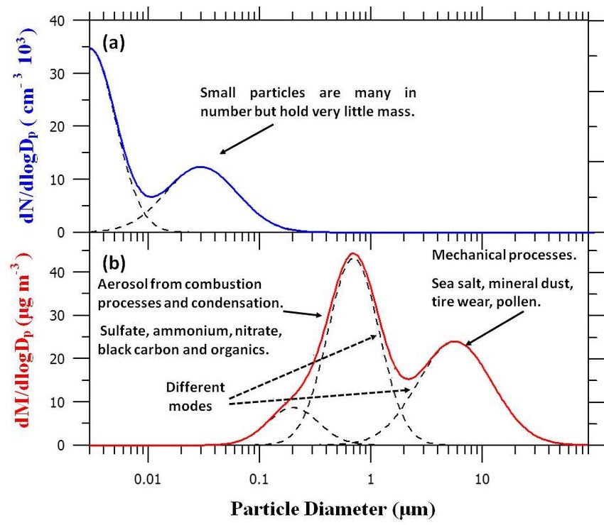
DNICast, Deliverable 2.2
Figure 11: Average frequency of African dust outbreaks across the
Mediterranean basin during the period 2001 - 2011 (Pey et al., 2013). ...... 26
Figure 12: Average global distribution of sulfur emissions from 2000 to 2007
(a) and corresponding optical depth (b) (Chin et al., 2009). ........................ 27
Figure 13: Average global distribution of black carbon emissions between
2000-2007 (a). The corresponding optical depth has been separated based
on BC sources into pollution (b), mainly due to fossil fuel combustion, and
biomass burning (c) (Chin et al., 2009). ........................................................ 29
Figure 14: Aerosol mass size distribution and light scattering coefficient
(550 nm) in Bejing during June 2009 (Bergin et al., 2001). .......................... 31
Figure 15: Graphical representation of atmospheric processes. ................. 32
Figure 16: Mass size distribution (a) as a lognormal distribution and (b) with
discrete number of size bins who’s composed is known. ............................ 35
Figure 17: Research dust forecast centers operating under the SDS-WAS
framework. The two regional nodes are depicted with blue arrows and the
corresponding forecast centers with dashed blue lines............................... 37
Figure 18: Flow of information between various SDS-WAS regional
components. ................................................................................................. 38
Figure 19: An instance of the continuously updated AOD forecast available
at the NA-ME-E web portal corresponding to noon of January 27th 2015. The
same color coding is applied on each surface graph. ................................... 40
Figure 20: Image acquired from a volume imaging Lidar. Boundary layer
depth and cloud height for different cloud types are shown. ..................... 43
Figure 21: Schematic diagram of the different physical processes
represented in the IFS model. ...................................................................... 45
Figure 22: Bias error of the simulated AOD550 against the AERONET
observations during April 2003. Dot size varies as a function of available
observations (Morcrette et al., 2009). ......................................................... 46
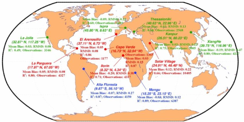
Figure 23: Map view of AERONET stations where the MACC-ECMWF model
was evaluated during 2003 - 2006. Sites are color-coded according to
expected aerosol type: urban/anthropogenic (green), biomass burning
(blue), and dust (red; Cesnulyte et al., 2014). .............................................. 47
Figure 24: Seasonal variation of the monthly average mean bias (MB)
obtained from the comparison between modelled versus direct-sun
AERONET AOD550 lumped based on region. M4 and M8 correspond to the
DREAM and BSC-DREAM8b models, respectively (Basart et al., 2012b). .... 50
9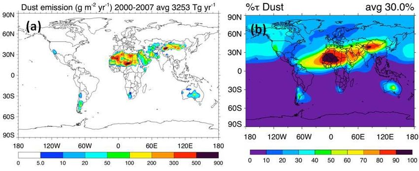
DNICast, Deliverable 2.2

Figure 25: Comparison of satellite (CALIPSO) and BSC-DREAM8b dust AOD550.
Color bar represents the latitudinal zone of the comparison,in 5° bins
(Amiridis et al., 2013). .................................................................................. 51
Figure 26: Comparison of modeled against measured yearly averaged dust
surface concentration in μg m-3 (b) with respect to 22 AeroCom stations (a)
the name of which is given in Huneeus et al. (2010). A statistical table
showing the performance of the comparison is also given (right). The table
includes in the following order, RMS (normalized RMS), bias (normalized
bias), correlation with respect actual (logarithmic scale) values and ratio of
modeled and observed standard deviation indicated as sigma (Perez et al.,
2011). ............................................................................................................ 55
Figure 27: Model derived AOD500 (solid lines) over the Bodele against
AERONET measurements (blue dots). Two different meteorological
configurations were applied (Haustein et al., 2012). ................................... 56
Figure 28: Model derived (solid line) and AERONET AOD500 (blue dots) along
with Angstrom exponent (black circles) during 16–22 May at various
locations (Haustein et al., 2012). At Zagora the comparison corresponds to
AOD440 (measured) and AOD550 (modeled). The Angstrom exponent is used
to indicate the dominant AOD source (values
DNICast, Deliverable 2.2

Figure 35: Time series of modeled (blue line) and AERONET (black line)
AOD550 monthly averages at (A) Dakar, (B) Capo Verde (C) Banizoumbou,
and (D) Solar Village during 2012/09-2013/09. The grey shaded area and
red vertical bars indicate the standard deviation of the modeled and
AERONET mean respectively (Lu et al., 2013). ............................................. 71
Figure 36: Monthly averaged modeled against satellite (MODIS Terra, a;
MODIS Aqua, b; MISR, c) AOD550 observations during 2000-2009 (Randles et
al., 2013) and yearly averaged simulated against AERONET (d) observations
with respect to AOD550 during 2000-2007 (Chin et al., 2009). The location,
shown color coded based on region, of the 173 AERONET sites used is
shown (e). ..................................................................................................... 74

List of Tables
Table 1: List of products available at the WMO SDS-WAS North Africa-
Middle East - Europe (NA-ME-E) web portal. ............................................... 39
Table 2: Characteristics of SDS-WAS data available for download .............. 41
Table 3: Seasonal and annual statistics obtained with CALIOPE satellite
LIDAR over Europe for 2004 at the EMEP/CREATE stations (Basart et al.,
2012a). The statistical parameters used are explained in the Appendix. .... 50
Table 4: List of domains and corresponding resolution where simulation by
CHIMERE has been implemented. ................................................................ 62
Table 5: Modal diameters in micrometers (μm) of ambient aerosol
constituents implemented by GOCART ........................................................ 73
Table 6: Features of SDS-WAS model products taken from each model’s
individual site. Only forecasted products related to DNICast are considered.
 ...................................................................................................................... 78
Table 7: List of commonly used NetCDF tools. A complete list is also
available........................................................................................................ 91

                                                                                                                      11
DNICast, Deliverable 2.2
1. Introduction
The purpose of DNICast is to improve the use of short term forecasts
(commonly called nowcasts) of direct normal irradiance (DNI) from a
combination of numerical forecast products and observations. Reliable
forecasts of DNI can increase efficiency of concentrating solar technologies
(CST) if used as a decision-making tool in operation management.
What factors influence DNI? Sunlight (incident solar radiation) travelling
through the Earth’s atmosphere interacts with gases and particles and is
electromagnetically scattered in all directions as well as absorbed. Thus, the
direct beam of sunlight impinging on the Earth’s atmosphere is reduced in
intensity. DNI is the irradiance on a surface perpendicular to the line of
sight from the observer to the center of the sun caused by radiation that
did not interact with the atmosphere. The total energy flux of the direct
beam reaching the ground (i.e DNI) and the remaining scattered solar
radiation is called global radiation. Global radiation is most commonly
measured by global surface radiation networks coordinated by the World
Meteorological Organization using pyrheliometer instruments. DNI cannot
be forecasted accurately from just global radiation observations or
forecasts. Accurate prediction of DNI involves, in addition to measurements,
monitoring and modeling of solar radiation, aerosol, and clouds. In
particular, forecast development requires dedicated measurements of DNI
for evaluation and validation.
In Figure 1, a schematic of the Earth’s global annual mean energy budget is
shown (Kiehl and Trenberth, 1997 and Trenberth et al. 2009). Incoming
solar intensity at the top of the Earth’s atmosphere is 341 Wm-2. For the
purpose of this project it can be considered a constant. The amount of
incoming energy reaching the Earth’s surface is 184 Wm-2, the net energy
absorbed and reflected by the surface. This energy is global radiation
impinging from all directions of the hemisphere. DNI is a portion of this. Of
the remaining 157 Wm-2 (the difference between top of atmosphere
incoming radiation and that reaching the surface), 74 W m-2 are absorbed
by gas-phase molecules in the atmosphere (water vapor and O3) and 4-5
Wm-2 by aerosols, yielding a total of 78 Wm-2. The remaining 79 W m-2 are
reflected (scattering process) by clouds, aerosol and atmospheric gases (see
also Chapter 2.1). Model simulations combined with satellite observations
indicate that clouds reflect 47.5 Wm-2 of the solar radiation back to space
and aerosols 7 Wm-2. If the atmosphere were void of clouds, the aerosol-
reflected radiation would increase to 11 Wm-2.
12DNICast, Deliverable 2.2
Figure 1: The Earth’s global annual mean energy budget between March
2000 and May 2004 (W m–2). The broad arrows indicate the schematic
flow of energy in proportion to their importance (Trenberth et al., 2009)
The large effect of clouds on DNI is evident. One need only step outside to
observe this. On a global mean basis, they are responsible for 30% of the
solar radiation that reflected back to space. In contrast to clouds, the effect
of aerosols on a global scale is smaller at ≈4.5%. It should be emphasized
that the global mean picture represented by Figure 1 varies tremendously
from region to region since aerosols and clouds are highly spatially variable.
They tend to concentrate in certain parts of the world (see Figure 4 below
for aerosol global variations) Europe and the Mediterranean region is one
of them with anthropogenic aerosols and Saharan dust aerosols much more
abundant than in vast regions of the southern hemisphere. Also, this energy
picture does not take into account that aerosols are cloud precursors (the
so called indirect effect). In other words, the cloud effect shown includes
clouds that derive from aerosols.
Forecasting for instance on time scales of DNI nowcasting, 0-4 hours is
possible by representing with equations the atmospheric processes that
govern the climate system. Because atmospheric processes are linked
(coupled) with each other, the solution of each equation may affect the
solution of the rest. In other words, solutions of a non-linear set of
differential equations are involved, which is possible by applying numerical
methods and the Navier-Stokes equation of motions to build atmospheric
models. Understanding how these models operate presupposes
familarization with some fundamentals concepts of atmospheric science
13DNICast, Deliverable 2.2
found in Chapter 2. The reader is introduced to aerosols and their
properties; how clouds are formed from aerosol; the interaction of
radiation with particulate matter and some background information in
numerical modeling. This chapter may be skipped by readers with aerosol
science background. In Chapter 2.1 the reader is introduced in basic
concepts related with the interaction of atmospheric-relevant particles with
solar radiation. Chapter 2.2 introduces the concept of atmospheric
particulate matter and in Chapter 2.3 it is explained how particles are
related with clouds. An example of aerosol impact on incident rations is
presented in Chapter 2.4. A discussion concerning mineral dust, the most
abundant aerosol over land in terms of mass, can be found in Chapter 2.5.
In Chapter 3.1, atmospheric models are introduced. They simulate and
integrate complex atmospheric processes. In Chapter 3.2 the role of the
Sand and Dust Storm Warning Advisory and Assessment System (SDS-WAS)
with respect to dust simulations is explained and information on how to
retrieve forecasted AOD from a suite of atmospheric models is provided. In
Chapter 4 ground stations and satellite measurement techniques, relevant
to DNICast are reviewed. The final chapter 5 of this work is a
comprehensive review of dust simulation models involved in SDS-WAS, that
includes a summary of each model and comparison of the forecasted
variables against observations either from ground stations or satellites. For
each model’s review, the final chapter is dedicated in providing information
and links of the online available data that can be retrieved from each model.
Chapter 5 concludes by presenting some practical examples that explain
how the content of this work can be of use to a CSP operator.
Because the DNICast project combines experts both from the concentrating
solar technologies and from the meteorological sector, this document does
not assume prior knowledge of atmospheric processes necessary to follow
the content of Chapter 3, 4 and 5.
2. Basic Concepts
2.1 Interactions of Radiation with the Atmosphere
2.1.1 Beer-Lambert Law
Gases, aerosols, or clouds found in the atmosphere can absorb and scatter
incident radiation. The combined effect of scattering and absorption is
called extinction. The reduction of incident radiation intensity due to
extinction along a path (vertical or slant) is given by the Beer-Lambert law
(Eq. 1).
F ( ) F0 ( ) exp(bext ( ) z ) Equation 1
14DNICast, Deliverable 2.2
where F and F0 are the intensity of the beam at the bottom and top of the
path in W m-2, respectively, z corresponds to the height of the path
(typically vertical path), λ is the wavelength of incident radiation and bext
the extinction coefficient (or attenuation) which is the fractional depletion
of radiance per unit path length. The extinction coefficient is a measure of
extinction efficiency. The type of electromagnet interaction with particles
and gases depends on the size of the particle (or gas) and the wavelength of
incident radiation. Fig. 2 shows the solar spectrum and the colors making up
visible light. The extinction coefficient, and hence the efficiency of
extinction, changes with wavelength depending on type of scattering.
Scattering by very small particles and atmospheric gases of a size much
smaller than the wavelength of visible light (λ) is described by Rayleigh
scattering which is dependent on λ-4. Blue light is the shortest in the visible
spectrum and is scattered by gases more effectively than yellow and red
light. As a result, blue reaches the observer at the Earth’s surface better
than yellow and red and the sky is perceived as blue.
Figure 2: Solar radiation reaching Earth’s surface. The UV, visible and
infrared parts of the spectrum is depicted. The coloring of the visible part
of the spectrum is also shown.
Scattering by atmospheric aerosols whose size is comparable to the
wavelength of light is described by Mie theory of electromagnetic radiation
interaction with particles and depends on λ-1 (Seinfeld and Pandis, 2006).
Scattering by aerosols is most efficient when the diameter of a particle is
close to the wavelength of the incident radiation. However, maximum is
typically observed at sizes lower than the wavelength of incident radiation,
15DNICast, Deliverable 2.2
because the particles’ composition also affects its scattering efficiency
(Seinfeld and Pandis, 2006). An example is shown in Figure 3, where the
extinction coefficient of ammonium sulfate particles, shown as a function of
size, for incident radiation with wavelength equal to 550 nm, maximizes at
approximately 500 nm.
Figure 3: Dependance of volume-normalized single particle cross section
as a function of particle size for a particle with refractive index equal to
1.5±0.02i (Willeke and Brockmann, 1977).
2.1.2 Optical Depth
If thick smoke appears between an observer and a bright light, the light
appears dim because the extinction coefficient of smoke is greater than
that of clean air. Even when smoke is not present, the light source will also
appear dimmer to the observer but only if the distance from the light
source is greatly increased. This is because Rayleigh scattering of gas
molecules is much less than Mie scattering of smoke particles.
Another example is the color of the sun. The sun is white, but is perceived
as yellow from the Earth’s surface due to extinction from atmospheric
components. During sunset, solar beams travel greater distances to reach
the Earth’s surface than at noon (i.e. z in Eq. 1 increases) and extinction of
blue and green wavelengths are also greater. As a result red reaches the
observer more easily and the sun appears red.
16DNICast, Deliverable 2.2
In order to express extinction easily, a non- dimensional variable named
optical thickness (τ) is defined. It is the integrated extinction coefficient
over a vertical column of unit cross section (Eq. 2a) and corresponds to the
degree an incident beam is absorbed or scattered.
( ) bext ( )dz Equation 2a
z
The combination of Eq. 1 with Eq. 2a yields
F F0e Equation 2b
In Eq. 2b, where F is intensity of light observed and Fo is intensity of direct
beam incident light, the meaning of optical thickness is evident; a value of
optical thickness 1 means that direct beam light is attenuated to 1/e of its
original value. In other words, there is a 63.2% attenuation of the original
direct beam of light after passing through a layer of air with optical
thickness equal to unity.
According to the strict definition of the American Meteorological Society
(AMS) in the Glossary of Meteorology, optical thickness at a particular
wavelength gives the line integral of extinction along any line of sight (e.g
observer’s eye to the sun), while optical depth is the optical thickness (AOD)
projected onto a vertical path. This definition is consistent with terminology
used by the World Meteorological Organization’s Guide to Meteorological
Instruments and Methods of Observation. We caution the reader to beware.
In many published papers in the literature including those from the space
agency NASA, the term Aerosol Optical Thickness or AOT is used
synonymously with Aerosol Optical Depth or AOD. In this report, we shall
use AOT and AOD according to the international standard definition.
Radiation interacts with a variety of atmospheric gases as well as aerosols.
These include ozone (O3), carbon dioxide (CO2), water vapour (H2O) or
absorbing trace gases (eg NO2, chlorofluorocarbons). For each component
an optical depth can be defined and their sum equals the total optical depth
(Eq. 3).
( ) aerosol clouds O CO H O other
3 2 2
Equation 3
Usually in the atmosphere, the total column concentration of longer lived
gases such as CO2 and O3 do not change on timescales shorter than the
nowcasting horizon of DNICast, which is four hours. However, the aerosol
and cloud optical depths or thicknesses may undergo large variation and
are considered important variables to nowcast DNI.
17DNICast, Deliverable 2.2
As mentioned above, Mie scattering of sunlight by aerosols is more
effective if the particle’s size is comparable to the wavelength of light. This
means that optical depth is wavelength and aerosol size distribution
dependant.
Figure 4: A best estimate of the global distribution of annual average
tropospheric aerosol optical depth (AOD 550 nm) compiled by combining
data from six satellites operating for limited periods between 1979 and
2004 (courtesy of S. Kinne MPI, Hamburg, Germany).
Fig. 4 shows the global distribution of the annual average tropospheric AOD
derived from multi-year observations from six satellites evaluated using
surface based observation of AOD using suntracking sunphotometers such
as those in the AERONET, SKYNET and WMO/GAW PFRNET network. This
represents extinction by all aerosol types but certainly sand and dust
aerosol extinction over and downwind of North Africa and the Middle East
as well as the central Asian deserts are evident.
The satellite signal depends on the combined effect of the Earth’s surface
reflectance with that of clouds, aerosol and gas molecules. Images are
acquired at several wavelengths (blue, green, red, and near-IR) that result
in practically scanning the whole visible spectrum. Algorithms are applied to
mask out the effect of scattering by air molecules (Vermote et al., 2002)
and the acquired images use wavelengths where atmospheric gases do not
absorb. Clouds are also masked, but their presence complicates AOD
retrieval. Thick clouds obscure underlying surfaces, while thin (cirrus)
18DNICast, Deliverable 2.2
clouds are difficult to identify. Cloud edges are not easily discernible and
cloud shadow poses another complication for retrieving the Earth’s
reflectance. Earth’s colorful surface which is comprised of grass, land, rocky
Mountains, deserts and oceans constitutes background noise for AOD
retrieval. Because oceans mainly absorb solar radiation, it is assumed that
all reflected radiation is caused by aerosols. Hence AOD over the oceans
can be accurately determined. Areas where the Earth’s reflectance is higher
(deserts, rocky terrain) AOD retrieval is more uncertain.
2.1.3 Other characteristic optical properties
In order to fully characterize the optical properties of aerosol, cloud
droplets and ice crystals two variables, additional to the extinction
coefficient, are used. The single scattering albedo ω(λ) provides information
on the contribution of scattering to the total extinction and hence the
relative importance of scattering and absorption. It is the ratio of scattering
to extinction and therefore cannot exceed unity. A single scattering albedo
equal to unity means that only scattering takes place, while a value of zero
that only absorption occurs.
When light is directed onto a mirror the beam’s direction will change at a
fixed angle. When a beam interacts with a particle or cloud droplet, it will
be scattered in all directions (360°). If light is scattered equally amongst all
directions then it is called isotropic scattering. This is the case in the
Rayleigh scattering regime which involves gases. However, for scatterers of
greater size (e.g. aerosol) light is scattered non-uniformly. In order to
account for this phenomenon, the asymmetry factor (g) is introduced. The
asymmetry factor is defined as the intensity-weighted average cosine of the
scattering angle and may vary from +1 to -1. Positive values indicate that
forward scattering is favored while negative values that backscattering is
favored. When isotropic scattering occurs the asymmetry factor is equal to
zero.
2.2 Fundamental Aerosol Properties
2.2.1 Particle size is linked with emitting source
Solid or liquid particles suspended in air are commonly called aerosols by
atmospheric scientists. A key property of these particles is their size
(typically the particle diameter is used), which spans five orders of
magnitude from a 10-3 to 10 micrometers (μm). Particles with diameter
greater than 0.1 μm represent a small fraction of the total number of
particles yet hold almost the entire particle mass. Particles with diameter
smaller than 0.1 μm are orders of magnitude more in number but hold very
19DNICast, Deliverable 2.2
little mass (Fig. 5a). Dividing the particle size range into discrete intervals
and sorting according to some property such as number, surface area or
mass is commonly practiced since aerosol impacts optically or on human
health (when inhaled) depend strongly on size distribution.
Figure 5: Typical number and mass distributions of atmospheric particles.
Different modes are depicted in the graph. Because particle diameters
span several orders of magnitude, the x-axis of the graph is in logarithmic
scale (Seinfeld and Pandis, 2006).
The composition of atmospheric particles is very size dependent. A typical
mass size distribution, shown in Fig. 5b, includes two modes (peaks). Each
mode corresponds to a different particle source. Particles with diameter
smaller than 1 to 2.5 μm are commonly referred to as fine particles. The
size cut varies from science community to community. Particles are
primary, resulting from direct emission from sources to the atmosphere, or
secondary, produced from gas to particle conversion. The latter happens
when atmospheric gases chemically react to produce involatile molecules
that condense with each other, other molecules and on surfaces. They can
come from both natural sources (e.g. dimethyl sulfide gas from marine
sources, volatile organic compounds from vegetation, forest fires,
volcanoes), or anthropogenic sources (e.g. fossil fuel combustion, smelting).
20DNICast, Deliverable 2.2 Particles with diameter greater than 1 to 2.5 μm and less than 10 μm, are typically referred to as coarse particles. They are the result of mechanical processes at the Earth surface (Seinfeld and Pandis, 2006). Sea salt particles and mineral dust, both of which are of interest in DNICast due to their scattering properties, fall in this category but also can contribute to fine particulate matter. Sea salt particles (sea spray) derive from the suspension and evaporation of sea water droplets from jet and film drops formed when air bubbles burst in the whitecaps of stormy seas. A solid particle, formed by crushing or other mechanical action that results in physical disintegration of a parent material is called dust (Kulkarni et al., 2011). Anthropogenic sources that fall in this size category are tire wear particles and dust from human activities (e.g. mining) or from winds interacting with the Earth’s surface. Coarse particles also can contain gas to particle conversion products such as nitrates and organics but to a lesser extent than fine particles. Coarse particles with diameters greater than 10 μm settle very fast and hence have relatively short lifetimes in the atmosphere unless they are lifted to very high altitudes by strong vertical winds. Particles larger than 10 μm are of little interest for optical extinction. 2.3 Cloud Condensation Nuclei (CCN) Atmospheric aerosols play a key role in cloud formation. If the atmosphere were void of particles, relative humidity (RH) would need to be very supersaturated (e.g. RH >200%) in order for liquid cloud droplets to form by homogeneous nucleation of liquid water and condensation. This is not the case in the atmosphere where super-saturations of 1% are more typical. This is because water readily condenses onto hygroscopic particles forming clouds at RH slightly above 100%, a process named heterogeneous nucleation. No particles can be activated (i.e. form a cloud droplet) at sub- saturated conditions (RH
DNICast, Deliverable 2.2

of liquid water cloud droplets. Fig. 6 shows the Atlantic Ocean covered with
human altered clouds that appear as white lines in contrails emitted by
ships burning fossil fuels.
Even if RH exceeds 100%, not all particles are activated. The ability of a
particle to serve as a cloud condensation nuclei (CCN), depends on its size
and composition. Aerosols composed of water soluble constituents (e.g.
salts or acids of sulfate, nitrate, or chloride) are hygroscopic and favored as
CCN. At high altitudes, temperatures are well below 0 °C. Unlike bulk water,
liquid cloud droplets do not readily freeze at 0 °C resulting in clouds with
supercooled liquid water droplets, ice crystals or both together (Fig. 7). To
form ice in droplets the size of cloud droplets (1 to 100 μm diameter)
requires either homogenous nucleation of ice by clusters of water
molecules or heterogeneous nucleation by aerosols. Homogeneous
nucleation of water in cloud droplets requires temperatures below -40 °C
while heterogeneous nucleation by certain types of aerosols (e.g. clay
minerals found in windblown dust) can occur at temperatures close to 0 °C.
In practice observations show that real clouds are found to have
progressively more ice as temperatures decrease (Fig. 7). The physical state
of a cloud determines its radiative properties such as brightness. For the
same total water content, ice clouds are more transparent to radiation
(optically thinner) than water clouds. Thus, aerosols acting as cloud
condensation nuclei or as ice nuclei influence microphysical properties that
determine the interaction of a cloud with radiation.

Figure 6: Ship tracks (white lines) in marine stratus clouds over the
Atlantic Ocean as viewed from satellite on January 27, 2003. Brittany and
the southwest coast of England can be seen on the upper right side of the
image (Wallace and Hobbs, 2006)

                                                                            22
DNICast, Deliverable 2.2 Figure 7: Variation of the frequency of supercooled clouds and of clouds containing snow crystals. Curves (1) and (2) pertain to ordinate on the left; curves 3 to 6 pertain to ordinate on the right. (1) Peppler (1940) over Germany, (2) Borovikov et al. (1963) over the ETU, (3) Mossop et al. (1970) over Tasmania, (4) Morris & Braham (1968) over Minnesota, (5) Isaac & Schemenauer (1979) over Canada, (6) Hobbs et al. (1974) over the northwest United States (Pruppacher and Klett, 1997). 2.4 Aerosol constituents and sources 2.4.1 Sea salt Sea salt is formed from evaporation of sea spray which results mainly from air bubbles bursting over whitecaps in marine areas at surface wind speeds of 4 m s-1 or higher. Production increases exponentially with wind speed above this threshold. At elevated wind speeds, much greater than 4 m s-1, wave crests are directly broken up by wind and thus form sea spray droplets and upon evaporation, sea salt particles larger than those formed by the bubble bursting process. Sea salt is ubiquitous over the ocean and nearby (0-20km) coastal areas as shown in the emission sea salt map on Fig. 8. Several different parameterizations concerning sea spray production have been used in modeling sea salt aerosol generation (Monahan et al., 1986; Gong et al., 1997; Vignati et al., 2001; Gong, 2003) which are reviewed and summarized by Ovadnevaite et al. (2013). Although sea salt aerosol aerosol optical depth (AOD) over land is generally low (
DNICast, Deliverable 2.2

and therefore affect cloud optical properties such as reflectivity of sunlight.
Thus, the effect of sea salt on clouds needs to be incorporated into models.

Figure 8: Average global distribution of sea salt emissions between 2000-
2007 (left) and percentage contribution of sea salt to global AOD based on
model simulations (right) (Chin et al., 2009)
2.4.2   Mineral Dust
Another very abundant natural aerosol is windblown dust, which can be
mobilized either by anthropogenic activities (mining, suspension due to
road traffic) or more commonly naturally by high winds in arid regions. Dust
typically refers to soil particles whose diameter can be up to 1 mm (103
μm). These large particles settle fast due to gravitational forces and in
practice only those with diameters smaller than about 100 µm can be
suspended in air. Horizontal transport and vertical transport in the
atmosphere is possible for particles of even smaller size (
DNICast, Deliverable 2.2

windblown dust particles than silt soil, which in turn produces smaller
particles than sandy terrains. Soil erodes only if it is dry, therefore a key
parameter controlling dust production is the soil moisture content, which
varies throughout the year and its calculation is a major issue and source of
error in atmospheric dust modeling.

Figure 9: Average global distribution of dust emissions between 2000 -
2007 (a) and corresponding optical depth (b) (Chin et al., 2009).
In order for dust to be lifted, wind speed must exceed a threshold value
(UCAR/COMET, 2010) that varies with soil type and terrain characteristics.
Three major dust mobilization mechanisms are “suspension”, “saltation”
and “creep” (Usher et al., 2003). These are depicted schematically in Fig. 10.
Sand blasting in high wind condition also breaks up large soil particles into
finer ones that can be more readily suspended.

Figure 10: Schematic representation of the wind-induced entrainment
processes to move, emit, and transport mineral dust particles (Usher et al.,
2003).
The suspension mechanism involves upward transport by turbulence in the
atmospheric surface boundary layer as well as convection and advection in
the free atmosphere. Fine particles may be transported to high altitudes (6–
8 km) and over distances of thousands of kilometers. This mechanism
involves particles smaller than 100 μm. The saltation mechanism involves
particles with diameters smaller than 500 μm. Wind currents lift particles

                                                                           25
DNICast, Deliverable 2.2
up to 1 m, but due to their big size are gravitationally pulled back to the
surface. Particles of size greater than 500 μm in diameter are transported
by the creep mechanism. They roll or slide along with the wind, impacting
particles on the land surface, favoring the movement of other particles.
According to the model estimates of Chin et al. (2009) windblown dust
particles contribute to approximately 30% of the global average AOD which
is greater than that of sea salt (15.7%). Due to the high variability of surface
winds, windblown dust concentrations in the atmosphere are very episodic.
They can increase very abruptly by a factor of 10 for a period of a few hours
to days. Dust outbreaks in the Mediteranean region are frequent several
hundred or even a thousand kilometers away from the sources in Northern
Africa (Pey et al., 2013, see also Fig. 11). The frequency decreases with
distance from the source region. As an example, at the Iberian peninsula a
dust outbreak is expected to occur once every 3 to 6 days on average. The
frequency is higher in southern Spain than in northeastern Spain or
southeastern France which is located further away from the dust source
(Fig. 11). These outbreaks, over the western Mediterranean are mainly
observed during summer, contrary to the eastern Mediterranean where
dust outbreaks are more often during autumn and spring (Querol et al.,
2009).
Figure 11: Average frequency of African dust outbreaks across the
Mediterranean basin during the period 2001 - 2011 (Pey et al., 2013).
26DNICast, Deliverable 2.2
2.4.3 Sulfate
Sulphates result naturally from primary particle and gas emissions from
volcanoes and oceans (Seinfeld and Pandis, 2006). Near source regions, sea-
salt sulfate is found mostly in the coarse mode in contrast to other sulphate
aerosols that that are produced in the atmosphere from oxidation of
sulphur dioxide or dimethyl sulphide and are generally found in particles
with diameters smaller than 1 μm. Sea salt sulfate is a primary aerosol
emitted directly into the atmosphere. It is commonly distinguished from the
remaining sources which are commonly called non-sea salt sulphate (NSS).
Sulphates also have large anthropogenic sources mainly related to gas to
particle conversion of sulphur dioxide gas. Sulphur dioxide is produced
during combustion of sulphur rich fossil fuels as well during the smelting of
sulphide based metal ores. It is emitted to the atmosphere where it is
oxidized to sulphuric acid and sulphate salts.
According to model estimates of Chin et al. (2009), natural plus
anthropogenic sulfate aerosols contribute more to global AOD550 than any
other aerosol type (Fig 12b). This is mainly because sulfates are associated
with sizes smaller than 1 μm, which are the most effective solar radiation
scatterers (Chapter 2.4). Strong source areas of sulfur gases precursors do
not necessarily correspond to high AOD (Fig 12a) partially due to the lag
between emission and oxidation to sulfate, which allows long range
transport of these pollutants.
Figure 12: Average global distribution of sulfur emissions from 2000 to
2007 (a) and corresponding optical depth (b) (Chin et al., 2009).
2.4.4 Organics
Organics originate from a myriad of sources including oxidation of biogenic
gases from forests and oceans, fossil fuel combustion, bacteria, pollen,
biomass burning, cooking, the surface ocean organic layer mobilized as sea
spray, tire wear and road dust. Together with elemental carbon, organic
27DNICast, Deliverable 2.2
matter constitutes the carbonaceous fraction of aerosols. Organic aerosol is
typically found in the fine mode and is the most abundant component with
respect to mass in that aerosol fraction (Kanakidou et al., 2005), followed
by sulfate. Organic aerosols are generally colorless, and similar to sulfate,
scatter radiation contribute greatly to scattering of light and hence DNI
reduction. They are a driving factor of particle growth to sizes where the
scattering efficiency maximizes (0.1-1 μm) thus enhancing the scattering
properties of dry particles. However, under atmospheric relevant conditions
that are typically humid, the scattering efficiency of particles has been
shown to decrease with increasing organic content because organic
substances tend to repel water (Zieger et al., 2014).
Absorption of these organic compounds, resulting in what is referred to as
brown carbon, is also of interest. Together with black carbon and dust,
brown carbon constitutes the three most important light absorbing aerosol
components. Unlike black carbon, which absorbs strongly in the mid-visible
spectrum (≈500 nm), brown carbon absorbs at wavelengths below 500 nm.
Its absorbance is an order of magnitude smaller than that of BC (Yang et al.,
2009), but its effect on climate is not negligible (Kirchstetter et al., 2004).
Because both brown and black carbon result from the same combustion
sources, they are typically found together and hence will be discussed
together in greater detail in Chapter 2.4.5.
2.4.5 Black carbon from biomass burning and fossil fuel emissions.
Black carbon results from the incomplete combustion of fossil fuels or of
biomass and is found with organic material in aerosols. Black carbon is the
most light-absorbing aerosol constituent. Its absorbance of sunlight is two
orders of magnitude greater than that of dust. Similar to most atmospheric
aerosol combustion products, black carbon particles occur in the fine
particle mode (Chapter 2.2.2) which scatters sunlight more efficiently than
larger dust particles. However, the mass loading of black carbon is also two
orders of magnitude less than that of dust. Thus, according to model
estimates of Chin et al (2009), their contribution to global AOD (27.4%) is
comparable to that of windblown dust (30%). They also do not generally
occur together in the Mediterranean region since North African dust
transport involves little influence of anthropogenic black carbon pollution.
In urban areas, biomass burning refers to wood combustion for residential
heating and in agricultural areas biomass burning is a means of waste
disposal or energy production. In rural India biomass is a major energy
source (Rehman et al., 2011). However the most abundant biomass burning
source is forest fires in the tropics and boreal regions of the northern
hemisphere. The net contribution of biomass burning to the global AOD
28DNICast, Deliverable 2.2
(550 nm) budget has been estimated to be 14.3% (Chin et al., 2009). Similar
to dust events, biomass burning is often episodic and in specific areas can
be the most significant AOD source. These areas are the Amazon forest and
South Africa (Fig. 13c), where additionally biomass is a primary energy
source. Due to the episodic nature of biomass burning, inter-annual
variations up to a factor of 3 have been observed with respect to the
aerosol mass concentration, posing a challenge to AOD forecast. This
problem is addressed by dynamic biomass burning emission inventories
based on satellite observations (Van der Werf, 2006) that update daily.
Black carbon emissions related with Europe, USA, and China, shown in Fig.
13a, result mainly from fossil fuel consumption, which is also a source of
black carbon rather than biomass burning which is secondary in proportion.
Industries in China use coal to produce energy, contrary to USA or Europe
where the trend is to substitute coal with less polluting oil or natural gas. As
a result, the emissions of anthropogenic black carbon in China are higher
than in Europe and North America.
Figure 13: Average global distribution of black carbon emissions between
2000-2007 (a). The corresponding optical depth has been separated based
on BC sources into pollution (b), mainly due to fossil fuel combustion, and
biomass burning (c) (Chin et al., 2009).
29You can also read