The Missing Home Buyers: Regional Heterogeneity and Credit Contractions
←
→
Page content transcription
If your browser does not render page correctly, please read the page content below
The Missing Home Buyers:
Regional Heterogeneity and Credit Contractions ∗
                                          Pierre Mabille†
                                            NYU Stern

                                     Job Market Paper
                             (click here for the latest version)

                                        January 14, 2020

                                               Abstract

          This paper studies how delayed home ownership from young buyers affects the
      transmission of shocks to housing markets. Using a panel of U.S. metro areas, I show
      that mortgage originations to young buyers have decreased more in regions with
      higher house prices over the past 15 years, despite credit standards varying only na-
      tionally. I develop and calibrate a regional business cycle model of the cross-section
      of housing markets consistent with these facts. Young buyers have more debt, and
      credit constraints bind more in high-price regions. Therefore an aggregate tightening
      of loan-to-value and payment-to-income requirements generates heterogeneous local
      responses in home ownership and prices. This channel explains 86% of the cross-
      sectional differences in originations and 50% of the differences in house price declines
      in 2007-12. Regional heterogeneity dampens the effect of subsidies like the First-Time
      Homebuyer Credit, because they fail to stimulate high-price regions which suffer the
      largest busts. Credit relaxation policies achieve larger stimulus and welfare gains.

         JEL classification: E32, E60, G11, G12, G21, G28, G51, J11, R10, R20, R30
      Keywords: Dynamic spatial equilibrium, regional business cycles, household finance,
      mortgages, first-time buyers, home ownership, house prices, subsidies, Millennials

   ∗ I am extremely grateful to my advisors Stijn Van Nieuwerburgh, Mark Gertler, Virgiliu Midrigan, and
Stanley Zin for their guidance and support. I also thank Corina Boar, Gideon Bornstein, Jarda Borovicka,
Gian Luca Clementi, Andres Drenik, Vadim Elenev, Niklas Engbom, Jack Favilukis, Raquel Fernández, Si-
mon Gilchrist, Arpit Gupta, Walker Henlon, Kyle Herkenhoff, Fatih Karahan, Pavel Krivenko, Donghoon
Lee, Davide Melcangi, Kurt Mitman, Abdoulaye Ndiaye, Andrea Tambalotti, Wilbert van der Klaauw,
Laura Veldkamp, Venky Venkateswaran, Olivier Wang, and Mike Waugh for many helpful comments and
discussions, as well as seminar participants at NYU and the Federal Reserve Bank of New York. I thank the
Federal Reserve Bank of New York and Recursion Co for their provision of data. I gratefully acknowledge
financial support from the PhD Dissertation Internship of the Federal Reserve Bank of New York and the
Macro-Financial Modeling Group of the Becker-Friedman Institute.
   † Email: pmabille@stern.nyu.edu. Website: https://www.pierremabille.com/research.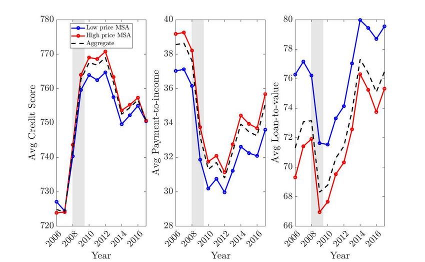
1      Introduction
A central feature of housing busts is their unequal incidence across demographic groups.
After 2007, the decline in young home ownership, a four decade-old trend, dramatically
accelerated and especially affected the Millennial cohort (Figure 1). It has attracted con-
siderable attention from policymakers and the mortgage industry, as its effects on hous-
ing markets and buyers’ welfare are still unclear. While it has been attributed to the lack
of housing affordability, it has also been blamed for the slow recovery of some housing
markets, two major features of the post-Great Recession period.1
     This paper studies the causes of delayed home ownership from young buyers and
how it affects the transmission of shocks to housing markets. In particular, it seeks to
explain how it coincided with a large dispersion in house price busts between regions
after the Great Recession – a puzzling fact for frictionless models of asset market partici-
pation where entering buyers should arbitrage price differences away. Jointly explaining
these facts is important both because of the quantitative importance of young buyers and
regional heterogeneity, and their potential implications for housing policies.2
     I show that delayed home ownership from young buyers is a channel which explains
differences in housing busts between regions when credit contracts. Because young buy-
ers tend to have lower income and little savings, they largely rely on mortgages when
buying homes. Because they are more credit-constrained in areas with higher house
prices, they disproportionately respond to changes in mortgage standards by delaying
home ownership. This, in turn, leads to larger price declines in those regions, dampening
the effect of housing stimulus policies conducted at the aggregate level.
     Using data on first-time buyers, I motivate this channel by documenting two new sets
of facts on mortgage originations in a panel of U.S. metropolitan statistical areas (MSAs).
First, originations to young buyers decreased by 40% more and house prices by four times
more in high-price MSAs than in low-price MSAs in 2005-17. Households delayed home
ownership more in high-price MSAs, where the average age of first-time buyers increased
from 35.5 to 37.5 years while it remained stable elsewhere. Young home ownership de-
    1 SeePiskorski and Seru (2018) and Goodman and Mayer (2018). Numerous examples include central
banks (“Coming of age in the Great Recession”, Federal Reserve Board speech by Gov. Brainard, 2015),
Government-Sponsored Enterprises (“Resolving the Millennial homeownership paradox”, Fannie Mae,
2018), think tanks (“Millennial homeownership: Why is it so low and how can we increase it?”, Urban
Institute, 2018), and banks (“Millennials: the housing edition”, Goldman Sachs, 2014).
   2 First-time buyers account for 50% of all purchase mortgages originated every year (Consumer Credit

Panel, New York Fed). On the refinancing channel of monetary policy, see e.g. Beraja, Hurst and Vavra
(2019a) and Wong (2019). On housing subsidies, see Berger, Turner and Zwick (2019).

                                                  1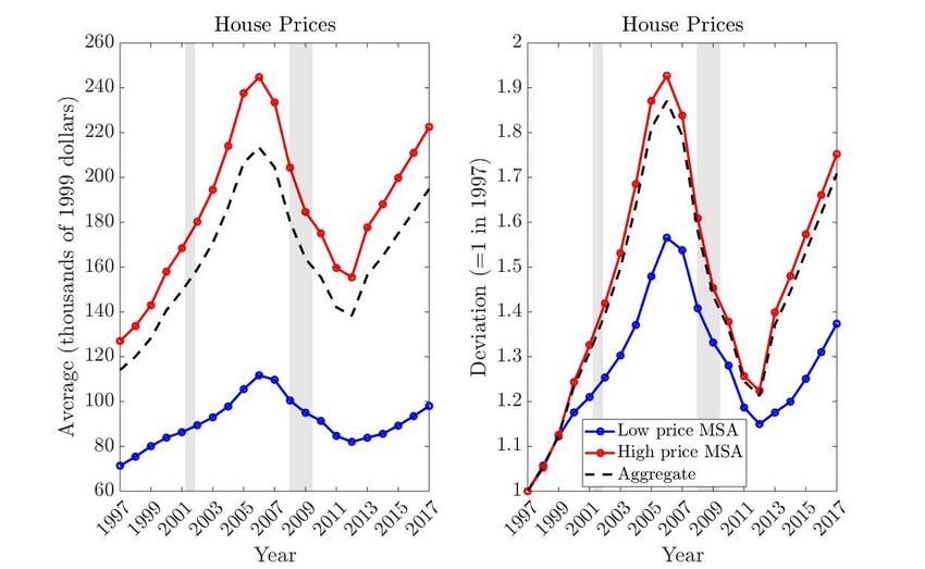
Figure 1: Changes in home ownership by age group

Source: American Community Survey. Values normalized to 100 in 2006 to view changes. Gray band indicates NBER recession.

creased by 70% more, leading to an increase in the regional dispersion of home owner-
ship. Second, this has been the case despite mortgages standards varying only nationally
over this period, with little regional variation in the characteristics of originated loans.
    I then develop an equilibrium regional business cycle model with housing markets
consistent with these facts. Regions in the model differ in the amenity benefits that hous-
ing provides, the cost of residential investment and the price-elasticity of housing supply,
and their exposures to nationwide income shocks. Each region is populated by overlap-
ping generations of risk-averse households who face idiosyncratic income and mortality
risks, and make discrete decisions on where to locate and whether to be renters or own-
ers, subject to credit constraints. When born, households also face different aggregate
environments which cannot be insured away and reflect cohort-specific characteristics.
    The key novel features are that (i) the regional distribution of house prices responds
endogenously to local and aggregate shocks, and (ii) households sort across regions based
on their individual characteristics.3 Their interaction gives young buyers a key role in
the transmission of shocks to housing markets. Regional heterogeneity induces older
and richer households to sort into high-house price MSAs. Sorting, however, is limited
by the low degree of regional mobility and the option to rent, which results in a large
fraction of young and poor households living in high-price MSAs. Because of higher
price levels, young households tend to delay home ownership and to be more credit-
constrained when buying. As a result, a nationwide tightening of mortgage standards
   3 Existingregional business cycle models assume exogenous house prices and no household mobility
(e.g. Hurst, Keys, Seru and Vavra (2016), Jones, Midrigan and Philippon (2018), Beraja et al. (2019a)). My
paper is the first to solve for the evolution of the regional distribution of prices, bringing these models
substantially closer to the data.

                                                              2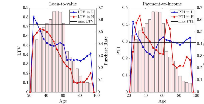
generates a larger drop in their home ownership in high-price regions than in low-price
regions. In equilibrium, this leads to a larger price decline in high-price regions because
the housing stock is durable and residential investment is irreversible.
    To discipline regional heterogeneity in the model, I map it to the panel of U.S. MSAs
constructed earlier. I estimate the parameters governing local housing market character-
istics using regional and micro data, and use the calibrated model to quantify the effects
of regionally binding credit constraints. I develop a new solution method for this class
of regional models, to compute the transition dynamics of the house price distribution in
response to unanticipated shocks. Using this framework, I obtain three results.
    First, the transmission of aggregate credit shocks through young buyers explains 50%
of the differences in house price declines between low- and high-price MSAs in 2007-12.
A realistic symmetric tightening of loan-to-value (LTV) and payment-to-income require-
ments (PTI) replicates the 10% decrease in young home ownership in low-price MSAs,
and the 20% decrease in high-price MSAs. It generates a 10% and a 20% decrease in
house prices in these MSAs, versus 10% and 40% in the data.4 More binding credit con-
straints lead to higher volatility in high-price MSAs, a feature of the data which has been
attributed to housing supply restrictions so far, but has remained puzzling for regions
where such restrictions are unlikely to apply.5 To illustrate the role of local house price
levels for credit constraints, I study a counterfactual economy with the less heterogeneous
house price distribution of 1997. The effect of regional credit constraints is muted: in re-
sponse to the same credit contraction, the house price busts in the low- and high-price
MSAs would have been of the same magnitude, and the aggregate bust would have been
3.8 percentage points (pp) smaller.
    Second, I study the determinants of regionally binding credit constraints on young
buyers: first, the primitive parameters governing regional heterogeneity; then, the cohort-
specific features of young buyers in the 2010s. I estimate that, once accounting for regional
credit constraints, amenity differences contribute as much to heterogeneity in housing
busts as housing supply restrictions – in contrast to received wisdom.6 Amenities gener-
ate differences in the cross-section of house prices levels, which affect the extent to which
credit constraints bind across MSAs.
   4 Inthe last section of the paper, I show that these differences are further amplified by local shocks to
labor income and to households’ valuations for owner-occupied units.
   5 My explanation complements Nathanson and Zwick (2018), who focus on speculation in the “sand

states” (Arizona, California, Florida, Nevada).
   6 For instance, the view that housing supply restrictions are key in generating dispersion in house price

changes is central to the identification strategy in Mian and Sufi (2009).

                                                     3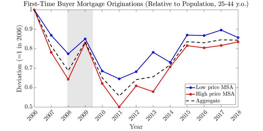
I find that worse initial conditions have persistently lowered the home ownership rate
of Millennials through their effect on wealth accumulation. I estimate that graduating
during the Great Recession has decreased their home ownership rate by 5.8 pp, and that
student debt has decreased it by 2 pp. However, with regional credit constraints, the
effect of initial conditions is more negative in high-house price MSAs, contributing to
decreasing long-run local prices (-8%). In contrast, they boost home ownership in low-
price MSAs and rental markets (+8%), as buyers either relocate to less expensive regions,
or stay longer in rental units.
   Surprisingly, initial conditions have not affected the volatility of housing markets by
making the Millennial cohort more sensitive to shocks. Their neutral effect on the pass-
through of shocks results from two counterbalancing forces. They make buyers more
likely to delay owning in recessions because of lower down payments and incomes; but
they also result in lower long-run prices, making credit constraints less likely to bind in
the first place. Here, the model demonstrates a dichotomy between the short-run and
long-run objectives of policies targeting young buyers: ameliorating their balance sheets
as they enter the housing market (e.g. with student debt relief programs) would improve
their home ownership, but it would not stabilize housing markets.
   Third, I evaluate the implications of regional credit constraints for the transmission of
housing stimulus policies. I study three policies targeting young buyers: (i) the First-Time
Homebuyer Credit (FTHC), a temporary tax incentive of $8,000 implemented in 2008-10;
(ii) a place-based version of the FTHC where housing subsidies are indexed to local house
prices; (iii) a credit relaxation policy. Table 1 summarizes their total welfare effects during
the recovery of the 2010s, in terms of consumption-equivalent variations. To validate my
results, I compare the treatment effects of the FTHC on home ownership and prices in
the model to identified empirical estimates, and show that they closely align. The FTHC
generates a persistent increase in aggregate welfare, due to improved access to home
ownership and a small increase in non-durable consumption.7 However, regional hetero-
geneity dampens its effectiveness, because a uniform subsidy fails to stimulate high-price
MSAs, which suffer the largest busts, and thus has a limited aggregate effect. Intuitively,
a “one size fits all” $8,000 dollar subsidy is more likely to relax buyers’ credit constraints
in low-price MSAs where the average house price is $120,000, than in high-price MSAs
where it is $217,000. Furthermore, the timing of distortionary taxes used to finance the
policy crucially affects the magnitude of the welfare gains, and can even reverse them en-
   7 I show that these results are robust to allowing for mortgage default, another source of house price

volatility which may have been suspected to dwarf the role of new buyers.

                                                   4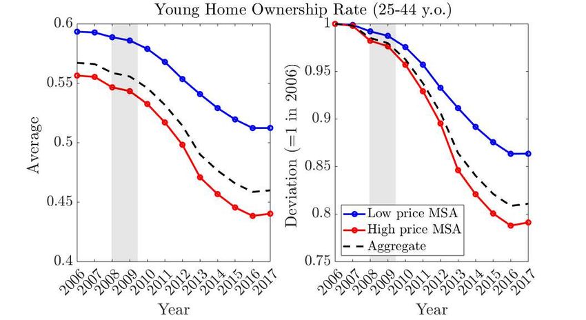
tirely if taxes are raised during the recovery period, an effect from which local treatment
effects in the empirical literature abstract.
    Owing to these limitations, a place-based version of the FTHC where buyers get $12,000
in high-price MSAs and $4,000 in low-price MSAs almost doubles aggregate welfare
gains. It stimulates young home ownership in high-price MSAs better, for the same dol-
lar cost. Of the three policies, a countercyclical relaxation of mortgage standards on new
buyers (during the recovery) achieves the largest welfare gains. Modeled after the 5 pp
increase in PTI requirements by Fannie Mae in 2017, the policy is a Pareto improvement,
with persistent welfare gains (up to the early 2020s). Those gains partly come from the
policy not being financed with distortionary taxes, partly from the fact that it directly re-
laxes credit constraints, and thus does not rely on comparing the dollar value of subsidies
to local house price levels.

          Table 1: Welfare gains from three stimulus policies targeting young buyers

                                                   FTHC        Place-based FTHC          PTI relaxation
                         Total welfare gain       +2.61%              +4.03%                 +6.05%

Notes: FTHC: First-Time Homebuyer Credit. PTI: Payment-To-Income requirements. Welfare gains are measured in terms of
consumption-equivalent variations (CEVs, in terms of the consumption of one four-year period). CEVs are computed for every house-
hold type, each period during the transition. They are aggregated using the time-varying cross-sectional distribution of households,
and summed across periods to obtain total welfare gains over the transition.

Related Literature
The analysis of the interaction of demographic characteristics and markets goes back to
Malthus (1798), and to Mankiw and Weil (1989) for the housing market. Recently, Glover,
Heathcote, Krueger and Rı́os-Rull (2017) and Wong (2019) have studied the effect of reces-
sions and of monetary policy on young buyers, while Ortalo-Magné and Rady (2006) have
demonstrated their contribution to aggregate house price volatility in a stylized model.
My contribution is to use a spatial setting to show that the larger effect of housing busts
on young buyers amplifies regional heterogeneity during recessions, and dampens the
transmission of stimulus policies. I contribute to three strands of the literature.
    First, the large regional heterogeneity in house prices changes is the basis for many
identification strategies in the empirical literature. For instance, Mian, Rao and Sufi (2013)
show that falling housing net worth negatively affected households’ consumption, and
Mian and Sufi (2014) that it led to lower employment. Guren, McKay, Nakamura and

                                                                 5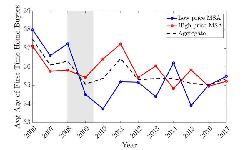
Steinsson (2018) do a similar exercise over a longer horizon. On firms’ side, Stroebel and
Vavra (2019) use these variations to study their effects on retail prices. Many of these
analyses rely on variations in local housing supply elasticities (Saiz (2010)) to instrument
for prices, implicitly adopting the view that supply restrictions are the main determinants
of differences in house price changes across regions. Much of the real estate literature
shares this view, with which Davidoff (2013) disagrees for the housing cycle of the 2000s.
My paper proposes a complementary explanation for regional differences in house prices
changes. It relies on the extent to which housing demand is constrained across regions
because of preexisting differences in house prices largely due to amenities. I show that
the large volatility in young buyers’ mortgage originations in high price MSAs, despite
identical regional variations in mortgage characteristics, lends empirical support to this
explanation. I share my focus on young buyers with a recent empirical literature studying
young home ownership during the 2010s, of which Acolin, Bricker, Calem and Wachter
(2016), Bleemer, Brown, Lee, Strair and van der Klaauw (2017), Goodman and Mayer
(2018), and Isen, Goodman and Yannelis (2019) are recent examples.8 I share my focus on
regional heterogeneity and the mortgage sector with Piskorski and Seru (2018), Gertler
and Gilchrist (2018), and Gilchrist, Siemer and Zakrajsek (2018).
   Second, my paper fits in the literature on regional heterogeneity and aggregate shocks.
Hurst et al. (2016) show that symmetric mortgage spreads across regions redistribute re-
sources to riskier regions and stabilize the economy in downturns. Beraja et al. (2019a)
demonstrate that regional heterogeneity in house prices dampens the refinancing chan-
nel of monetary policy. Based on differences between regional and aggregate responses to
shocks, Beraja, Hurst and Ospina (2019b) advocate the use of a structural model of U.S. re-
gions to draw inference about the drivers of business cycles. Jones et al. (2018) emphasize
regional credit constraints as drivers of fluctuations, a view that my paper adopts. My
contribution to this literature is to endogenize the distribution of regional house prices
and allow for sorting across regions. Lustig and Van Nieuwerburgh (2010) demonstrate
that the level of house prices affects households’ ability to borrow and insure against lo-
cal shocks through LTV constraints. I reverse their perspective, and show that different
house prices generate different binding constraints, which result in more heterogeneous
responses during recessions. While my paper focuses on changes between regions during
   8 Hurst(2017) and Foote, Loewenstein and Willen (2019) also stress the role of young buyers during the
Great Recession, and mention that they can potentially explain why the interpretations of the housing bust
by Mian and Sufi (2009) and Adelino, Schoar and Severino (2016) diverge. A separate literature on family
dynamics studies the trend towards low young home ownership, e.g. Fisher and Gervais (2011).

                                                    6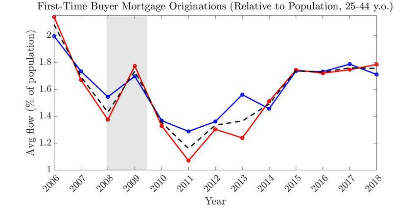
the bust, Landvoigt, Piazzesi and Schneider (2015) study changes within a region during
the boom, and show that a relaxation in credit led cheaper housing segments to appreciate
more. Finally, while several papers study monetary policy in regional models, my paper
instead analyzes housing subsidies and credit relaxation policies. Berger et al. (2019) con-
duct an empirical analysis of the FTHC, and Auclert, Dobbie and Goldmsith-Pinkham
(2019) study debt relief policies.
   Third, I contribute to the real estate and urban economics literature studying the deter-
minants of regional house prices, starting with Rosen (1979) and Roback (1982). Glaeser
and Gyourko (2005) show how amenities and supply constraints explain long-run differ-
ences in regional prices when housing is modeled as a durable good. Glaeser, Gyourko
and Saiz (2008) and Saiz (2010) show how differences in the price-elasticity of supply af-
fect the volatility of prices across regions. Mayer (2011) points to supply restrictions as
a prominent explanation for the volatility of historically cyclical regions, but notes that
it fails to explain the volatility of elastic regions in the 2000s, for which Nathanson and
Zwick (2018) provide an explanation based on speculation. Closer to the demand-side
channel that I propose, Van Nieuwerburgh and Weill (2010) relate the rising dispersion
in local house prices to the increase in regional income inequality. Like Guerrieri, Hart-
ley and Hurst (2013), I stress the role of amenities in driving house price levels and their
variations.
   More broadly, my paper relates to the literature on durable goods and housing, recent
examples of which include Berger and Vavra (2015), Rognlie, Shleifer and Simsek (2018),
Justiniano, Primiceri and Tambalotti (2019), Favilukis, Ludvigson and Van Nieuwerburgh
(2017), Kaplan, Mitman and Violante (forthcoming), and Garriga, Manuelli and Peralta-
Alva (2019b). I extend it by showing how regional heterogeneity affects the transmission
of shocks and policies.

Outline
The rest of the paper is organized as follows. Section 2 presents new facts on mortgage
originations to young buyers, and shows motivating evidence for the transmission mech-
anism formalized by the model. Section 3 presents the model, and Section 4 describes
the calibration that maps it to the panel of metro areas constructed in the empirical sec-
tion. Section 5 studies the transmission of aggregate credit shocks through young buyers,
and Section 6 studies the determinants of this mechanism. The implications for stimulus
policies are studied in Section 7, and Section 8 concludes.

                                             7
2 Mortgage Originations Across U.S. Regions
This section documents two new sets of facts on mortgage originations to first-time buy-
ers. First, over the past 15 years, mortgage originations to young buyers and their home
ownership have decreased more in high-price MSAs than in low-price MSAs. Second,
this has been the case despite mortgage underwriting standards varying nationally over
this period, with little variation in the characteristics of originated loans across regions.
2.1 Data Description
I construct an annual panel dataset of U.S. metro areas from 2001 to 2017 by merging data
on mortgage origination, households’ demographics and house prices from four main
sources. I use it to document stylized facts in this section, and later to calibrate the model.
I aggregate the data at the MSA level, the closest equivalent to local labor markets in
these datasets.9 Most weighted averages are computed using local population sizes as
weights, sometimes loan sizes. All nominal variables are expressed in 1999 dollars using
the BLS chained Consumer Price Index for all urban consumers.
First-time mortgage origination First, I use mortgage data on first-time purchase mort-
gages from the Federal Reserve Bank of New York Consumer Credit Panel (CCP). The
CCP is an individual-level, 5% random sample of the U.S. population with credit files
derived from Equifax. I use information on the number and balances of mortgages orig-
inated for all households and by age, aggregated at the MSA level. The data has infor-
mation on 370 of the 384 MSAs in the U.S. In the CCP, a first-time buyer is defined as the
first appearance of an active mortgage since 1999 with no indication of any prior closed
mortgages on the borrower’s credit report. Because first-time buyers are overwhelmingly
young households, using this variable allows to uniquely study the mortgages of young
buyers by merging the CCP with other loan-level datasets which do not have buyer’s age
as a variable. First-time buyers are quantitatively important: they represent 50% of pur-
chase mortgages, and have volatile mortgage originations. Those fell by 46% in 2004-11,
as much as for repeat-buyers.10
9 Analternative would be to construct variables at the Commuting Zone level using indications on zip
codes when they are available in the data. However this is not always the case.
10 The flow of loans originated to first-time buyers at the peak of the housing cycle in 2005 was 1.417
million, 665,000 at the trough in 2011, and 1.059 million in 2017.
8Loan underwriting standards Second, I combine the Single Family Loan-Level dataset
from Freddie Mac and the Single Family Loan Performance dataset from Fannie Mae, to
obtain information on the characteristics of loans issued to first-time buyers. I use the loan
origination and acquisition data to focus on originations. The Government-Sponsored
Enterprises loans (GSE) represent a subset of all purchase loans originated, but they were
the primary source of mortgage securitization for first-time buyers during the 2010s. I
focus on LTV and DTI ratios at origination, and borrower’s credit score. The total stocks
of loans are respectively 26.6 and 35 millions.
Household demographics Third, I use demographic information from the American
Community Survey (ACS) of the U.S. Census Bureau. I use information on MSA-level
total population, homeownership, age structure, migration flows, employment status and
median income by age at the household level.
House prices Fourth, I use Zillow’s Home Value Index (ZHVI) and Rental Index (ZRI)
for all homes and at the MSA level, as measures of median house prices and rents.11 The
data being monthly, I annualize it by taking the unweighted average across months in
a given year. The ZHVI is available from 2005 to 2017. The ZRI is available after 2010;
I extrapolate values from 2005 to 2010 by assuming that rents in each MSA grew at the
same rate as the U.S. consumer price index for rents from the BLS.12
2.2 Sorting Regions by House Price Levels
I start by sorting MSAs in two groups based on the level of house prices in 2006. In the
empirical and the model sections, I keep this classification of MSAs fixed, and study the
behavior of various variables within these two groups (e.g. the flow of mortgage origina-
tions). I denote MSAs in the bottom 50% of the distribution as “low-price MSAs” (in blue
in maps, graphs, and tables), and those in the top 50% as “high-price MSAs” (in red);
aggregate values are in black. This procedure is similar to Gertler and Gilchrist (2018),
who sort them by the severity of the local house price contraction after 2007. In fact, these
two classifications produce similar groups of MSAs, as many high price MSAs had larger
11 Iexperimented with repeat-sale house price indexes like the All-Transactions House Price Index of the
US Federal Housing Finance Agency and the S&P CoreLogic Case-Shiller Home Price Index. I obtained
similar results for the regional distribution of prices.
12 Consumer Price Index: Rent of Primary Residence in U.S. City Average, All Urban Consumers, Index
2010=100, Annual, Not Seasonally Adjusted.
9busts (and larger booms). Importantly, my results do not rely on the choice of the date at
which MSAs are sorted. Sorting them with the levels of 1997 house prices delivers iden-
tical results. This reflects the fact that some MSAs are historically more cyclical, and tend
to have higher prices (Mayer (2011)). My mechanism contributes to explaining why this
is the case.
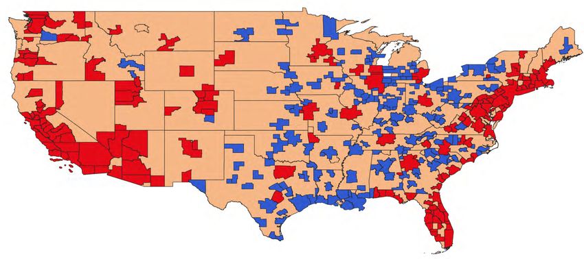
A detailed description of these MSA groups is in Appendix A.3. Figure 15 plots them
on a map and Table 11 lists them. Low-price MSA are concentrated inside the country
(for instance Indianapolis, IN, and Memphis, TN). High-price MSA are concentrated in
coastal regions and the Southwest (for instance Miami-Fort Lauderdale-Miami Beach, FL,
Phoenix-Mesa-Glendale, AZ, and San Francisco-Oakland-Fremont, CA). The first group
includes regions with historically stable house prices, with little construction restrictions,
and in low demand from buyers. The second group includes regions with a historically
higher volatility, which tend to have scarce buildable land, and regions with historically
stable prices which experienced high volatility during the 2000s. All regions in the second
group are in high demand from buyers.
Figure 14 in Appendix plots the evolution of the cross-section of house prices from
1997 to 2017. In 1997 the average price was $70,000 in the bottom 50% of the distribution,
and $120,000 in the top 50%. They increased less in low-price MSAs and more in high-
price MSAs during the boom (up to $110,000 and $240,000), and respectively fell less
and more during the bust (down to $80,000 and $160,000). Because high price regions
have more expensive homes and a large population, aggregate value- and population-
weighted price indexes (including median prices) track this group more closely. This will
be the case in the model too when aggregating MSAs.
House price differences induce sorting between the two MSA groups. High-price
MSAs have a 50% larger population, because they are on average more attractive and
productive (Mayer (2011)). However, sorting is limited. Despite house prices being 100%
higher, income in high-price MSAs is 10%-30% higher (median and average), and the
shares of young households (25-44 years old) and home ownership rates are identical
(ACS data). This is key for the transmission of credit shocks because it implies that buy-
ers have higher debt to income ratios in high-price MSAs.13
13 Otherhousing characteristics are similar, and thus unlikely to affect sorting between the two groups
of MSAs. The types of housing units are similar, and their sizes are only slightly lower in the more urban
high-price MSAs. The distribution of households by age and tenure status across unit types, number of
bedrooms, and building age is similar too (Appendix A.4). Relatedly, Sinai (2012) argues that demand
fundamentals account only for a small fraction of cross-sectional differences in housing busts.
102.3 Mortgage Originations to First-Time Home Buyers
Mortgage originations After sorting MSAs into low- and high-house price regions, I
document a first fact: mortgage originations to first-time buyers have decreased more in
high-price MSAs over the past 15 years after the recession. Figure 2 plots changes in the
average flow of purchase mortgages originated to first-time buyers (normalized by local
population) by region type and in aggregate. Averages are population-weighted.14
Figure 2: Mortgage originations to first-time home buyers by region
Notes: The solid lines depict changes in the average flow of mortgages originated to first-time buyers in low- (blue) and high-price
MSAs (red), relative to their populations. The dashed line depicts the economywide average. To view changes, their values are
normalized to 1 in 2006. Gray bands indicate NBER recessions. Source: CCP/Equifax, Zillow.
Delaying homeownership The decrease in first-time mortgage originations was associ-
ated with a temporary increase in the average age of first-time buyers in high price MSAs,
suggesting that many buyers delayed home ownership in unaffordable areas when credit
contracted (Figure 3). These findings complement Berger and Vavra (2015), who show
that buyers’ propensity to adjust housing vary over time. Here, I show that this margin
depends on local prices, and thus substantially varies across space.
14 This result is robust to weighting by the inverse of population of the total and of the young population,
to account for the larger population size of high price MSAs. It can also be seen by plotting the flow of
mortgages originated directly (Appendix A.6).
11Figure 3: First-time home buyer age by region
Notes: The solid lines depict the average age of first-time buyers in low- (blue) and high-price MSAs (red). The dashed line depicts
the economywide average. It is calculated as a weighted average using the number of loans at each age. Results are similar when
inversely weighting by the shares of each age groups in the MSA population (in the ACS), to account for changes in the age structure
of population across MSAs. Gray bands indicate NBER recessions. Source: CCP/Equifax, Zillow.
Rising dispersion in young home ownership The decrease in first-time mortgage orig-
inations resulted in a decrease in the entry rate into homeownership. It led not only to
a nationwide decrease in homeownership rates, which is well documented (Garriga, Eu-
banks and Gete (2018)), but also to an increase in their dispersion across MSAs for young
households (Appendix Figure 22).
2.4 Nationally Varying Credit Standards
What accounts for the large regional dispersion in mortgage originations to young buy-
ers? The second main fact that I document is that there has been little regional differences
in how credit standards have changed across MSAs over the last 15 years. Instead, as Fig-
ure 4 shows, credit scores, LTV, and PTI requirements tend to vary at the national level.
This finding is reminiscent of Hurst et al. (2016), who have documented the lack of spa-
tial variation in GSE mortgage spreads, despite observable regional heterogeneity. While
I am only able to show this fact in the Fannie Mae and Freddie Mac data, it is likely to
apply to all first-time buyers, as the GSEs and the Federal Housing Administration have
dominated the mortgage landscape since the recession. This findings also complement
Greenwald (2018) by showing that LTV and PTI ratios lack spatial variation.
12Figure 4: Average credit score, payment-to-income, and loan-to-value ratios at origination
across regions
Notes: Left panel: The solid lines depict the average credit score of first-time buyers in low- (blue) and high-price MSAs (red), when
their mortgages were first originated. The dashed line depicts the economywide average. Middle panel: average payment-to-income
ratio. Right panel: average loan-to-value ratio. Gray bands indicate NBER recessions. Source: Fannie Mae, Freddie Mac, Zillow.
2.5 Other Sources of Variations in Home Ownership
The symmetric tightening of credit constraints across MSAs, and the heterogeneous re-
sponses in the flow of mortgages originated (hence in young home ownership), are key
features of the data that my model will replicate. Appendix A.7 discusses alternative ex-
planations for these changes, including mortgage default, local credit supply shocks, and
the collapse of the private label mortgage securitization market.
2.6 Intuition: Regionally Binding Credit Constraints
I conclude the empirical section with a back-of-the-envelope calculation which illustrates
the mechanism that I formalize in the model. The mechanism incorporates the two facts
that I have documented: a symmetric tightening of credit standards across regions gen-
erates a larger decrease in mortgage originations (hence in young home ownership) in
MSAs with higher house prices. Therefore these MSAs experience larger price declines in
equilibrium. The core of the mechanism is that credit constraints bind more in high-price
than in low-price MSAs.
Consider the following calculations. Denote the mortgage rate as r b , the loan maturity
13as n, and LTV and PTI requirements by θ LTV and θ PTI . A simple mortgage payment
formula implies that the maximum loan size imposed by the PTI constraint is
1 − (1 + r b ) − n
PTI max loan size = θ PTI Y . (1)
rb | {z }
max payment each period
By definition, the maximum LTV loan size is θ LTV × price. Therefore the maximum house
price that households can afford is
" #
1 − (1 + r b ) − n down
max affordable price P = min θ PTI Y + down, . (2)
rb 1 − θ LTV
Figure 5 plots the maximum affordable price and the actual house price in each region,
feeding in time series for the empirical counterparts of the variables in Equation 2. While
the constraints are slack in low-price MSAs in 2006-17, they are clearly binding in high-
price MSAs. A decrease in the maximum affordable price is therefore associated with a
decrease in the actual price. However, these calculations abstract from many important
dimensions for housing markets, such as heterogeneity in households’ incomes and down
payments, the option to rent, the sorting of households’ across regions, and the interplay
of local and aggregate shocks. I therefore turn to a structural model of regional housing
markets to formalize and quantify this mechanism.
Figure 5: Regional credit constraints: maximum affordable price (P) vs. actual price (P)
Notes: Left panel: actual price (solid line) and maximum affordable price P (dashed line) in high price regions. Right panel: same
variables for low price regions. P is calculated using the formula in the main text, using r b = 5% (mortgage rate), n = 30 years (loan
maturity), and the path of average PTI ratios and median income in each group of MSAs (ACS data). Gray bands indicate NBER
recessions. Nominal variables are expressed in 1999 dollars.
143 Regional Business Cycle Model with Housing Markets
This section constructs a regional business cycle model of the cross-section of housing
markets. Its key novel feature is that the dynamics of the regional distribution of house
prices and rents is endogenous. I develop a tractable numerical method to exactly cal-
ibrate this class of models, and solve for price trajectories in response to unanticipated
local and aggregate shocks.
3.1 Environment
The economy consists of two building blocks. First, two sets of regions, low- and high-
price MSAs (j = L, H), are connected by migrations. Regional housing markets differ in
the amenity benefits they bring to households, the cost of residential investment, and the
price elasticity of housing supply. In this section, local labor markets are identical, and
households receive a stochastic endowment stream subject to idiosyncratic and aggregate
shocks (the latter are zero in steady state). In the last section, I extend the model to allow
regional endowment processes to differ in their exposures to aggregate income shocks.
Second, each set of regions nests a Bewley-Huggett-Aiyagari incomplete markets, het-
erogeneous agents economy. The economy is populated by overlapping generations of
households with a life-cycle. Population size is stationary, and there is a continuum of
measure 1 of households. Time is discrete.
Preferences Households have time- and state-separable preferences. They have a con-
stant relative risk aversion (CRRA) utility function over a constant elasticity of substitu-
tion (CES) aggregator of nondurable consumption ct and housing services ht . Amenity
benefits are modeled as additive utility shifters χ j , which depend on households’ regions.
A household’s instantaneous utility function in region j is
h 1
i 1− γ
1− γ
u (ct , ht ) ((1 − α)cet + αhet ) e
+ χj = + χj. (3)
1−γ 1−γ
Homeowners can own only one home, in a single size which delivers a fixed flow of
services h. Renters consume continuous quantities of housing services ht . χ j captures the
amenities accruing with different locations and the quality of the local housing stocks.
Bequests are accidental and not chosen by households, but there is a warm-glow bequest
15motive captured by the function
ψb1−γ
U (b) = . (4)
1−γ
For simplicity, bequests are a normal good, redistributed equally to all newborns.
Households’ choices Households can be either owners or renters. In each region, the
rental and the owner-occupied housing markets are partially segmented in that they give
access to different housing sizes. Owner-occupied units come in a single hsize ih at price Pj
in region j, and rental housing for type j can be chosen continuously in h, h at the rent
R j , with h being the minimum size. Every period, households can move between metro
areas, in which case they incur additive moving costs in terms of utility, m. They also
choose nondurable consumption ct , savings in one-period risk-free bonds or long-term
mortgage debt bt . They inelastically supply one unit of labor to the local labor market.
Endowments and risk Households face idiosyncratic income risk, and mortality risk.
The survival probabilities { p a } vary over the life-cycle. The law of motion for the log
income of a working-age household i, of age a, in region j is:
yi,j,a,t = ga + ei,t + β j ηUS,t
ei,t = ρe ei,t−1 + ε i,t (5)
iid
ε ∼ N µε , σε2
ga is the logarithm of their deterministic life-cycle income profile. ei,t is the logarithm
of the idiosyncratic, persistent component of income for household i. It has the same
persistence in the two regions.15 ηUS,t is the aggregate component of regional income,
which is zero in steady state. β j is the sensitivity of income in region j to aggregate income
ηUS,t . In the main version of the model β j = 1 for all j. In the last section β H > 1 > β L > 0.
The income process Yi,j,a,t = exp(yi,j,a,t ) is supermodular in regional and individual
income. The cross-derivatives
∂2 Yi,j,a,t ∂2 Yi,j,a,t
, >0 (6)
∂ β j ηUS,t ∂ga ∂ β j ηUS,t ∂ei,j,t
create a complementarity between the regional component, and the life-cycle and stochas-
15 The assumption of identical local income processes can be easily relaxed.
16tic components of individual income. Over the transition (when ηUS,t 6= 0), it creates a
motive for higher income households to live in regions with higher average income, gen-
erating spatial sorting.
Absent heterogeneity in β j , spatial sorting arises because of amenity differences. The
concavity of u makes it more costly for poorer households to sacrifice non-durable con-
sumption to enjoy better amenities in regions with higher house prices. This is a key
difference with urban economics models with risk-neutral households, which abstract
from wealth effects.
Taxes and transfers Labor income is subject to the progressive tax and transfer schedule
of Heathcote, Storesletten and Violante (2017),
T (Y ) = Y − ϕY 1−τ , (7)
where τ and ϕ respectively control the progressivity and level of taxes.
Retirement income is given by the pension schedule of Guvenen and Smith (2014),
which replicates salient features of the U.S. pension system (see Section B.1 in Appendix).
Households’ balance sheets Markets are incomplete, as households only have access to
a one-period risk-free bond with an exogenous rate of return r > 0 to smooth consump-
tion, and to houses.
Renters who are inactive face a no-borrowing constraint. Renters who buy can use
long-term mortgages to borrow, subject to LTV and PTI constraints, which only apply
at origination. They face an exogenous, kinked interest rate schedule, which makes bor-
rowing more costly, and comes from an unmodeled fixed financial intermediation wedge:
r̃t = r b > r if bt < 0, otherwise r̃t = r. Because r b > r, indebted households never simul-
taneously hold risk-free assets and debt, and prefer paying off their mortgages first. The
assumption that owners cannot save accounts for the large fraction of “wealthy hand-to-
mouth” households with little liquidity in the data (Kaplan and Violante (2014), Gorea
and Midrigan (2018)).
Mortgages are non-defaultable. In Section 7.4, I extend the model to allow house-
holds to default on non-recourse mortgages, to capture the exit margin of homeowner-
ship. When making this change, I assume that houses used as collaterals return to the
market upon default, that defaulters incur a utility penalty d, are forced to rent in the
same region, and return to the owner-occupied market in the next period with probabil-
17ity 1.16 Finally, owners cannot refinance and extract housing equity. 17
Cohort-specific initial conditions In the simulation, all agents enter the economy as
renters. They are divided into two categories based on the period in which they are born,
to capture cohort-specific features which affect housing markets. Households becoming
active on the housing market prior to 2005 draw a level of initial wealth equal to the
average bequest in the economy, and their initial income from the stationary distribution.
Households who become active after 2005 – Millennials – have two distinct features. First,
their levels of initial wealth are lower by a fixed amount corresponding to student debt
payments in the first three periods of their lives (from their twenties to their early thirties).
Second, when born during a recession, they draw their initial income from a distribution
which is first-order stochastically dominated by the baseline distribution, such that that
the recession has a negative, long-lasting effect on their earnings.
Housing supply The housing stock Hj,t in region j, in square feet, depreciates at rate δ:
Hj,t = (1 − δ) Hj,t−1 + Ij,t (8)
Residential investment Ij,t compensates for depreciation. At the household level, owners
pay a maintenance cost in dollars at the beginning of each period, δPj h.
The construction sectors in the two regions produce according to a reduced-form
upward-sloping supply curve,
ρj
Ij,t = I j Pj,t (9)
The housing supply elasticity ρ j , and the constraints on residential investment I j differ
across regions. The lower ρ j , the larger the price movements required to induce the same
change in residential investment in percentage terms. The lower Ij , the higher the price
level required to induce the same level of residential investment. Since households supply
labor inelastically, the construction sectors are only affected by price changes.18
Finally, the markets for owner-occupied housing and for rentals are segmented. Every
period, the housing stock Ht,j (in square feet) is exogenously divided into a fractions
sq f t sq f t
ho j of owner-occupied houses, and a fraction 1 − ho j of rentals, with no endogenous
16 In the model, this corresponds to a 4-year. It is also straightforward to allow for a different probability.
17 I consider this option in an ongoing extension.
18 It is straightforward to allow for time-varying region-specific shifters I , to capture regions’ different
j,t
cyclical sensitivities orthogonal to prices.
18conversion from one to the other. Appendix B.2 discusses this assumption in detail. As a
result, the supply of owner-occupied houses and of rentals (in square feet) are respectively
equal to
o sq f t r sq f t
Hj,t = ho j Hj,t and Hj,t = 1 − ho j Hj,t (10)
Timing A household in region j makes a discrete tenure and location choice, then earns
labor and financial income in its region of origin, and makes consumption, savings or
debt, and housing choices. I now turn to describing the households’ problem recursively.
3.2 Household’s Problem
The household’s individual state variables are its tenure status r, o (renter or owner), lo-
cation j = L, H (low-price or high-price region), age a, assets or debt b, and endowment
y. To save space I only describe the problems of households in the low-price region (L).
The problem is similar for the high-price region H.
3.2.1 Renter
Denote the date t value function of a renter of age a, with savings bt and income yt , who
starts the period in region L, as VtrL ( a, bt , yt ). First, a renter chooses the location where it
will move over the period, and whether to rent or own in its new location. The envelope
value of the value functions for each option is:
n o
VtrL ( a, bt , yt ) = max VtrL,rL , VtrL,rH , VtrL,oL , VtrL,oH (11)
Denote drL
t ∈ {rL, rH, oL, oH } the resulting policy function for the discrete choice
problem. After, renters choose their nondurable consumption, housing services, and sav-
ings, or mortgage debt if they borrow to purchase a house.
First, the value of being inactive and staying a renter in region L is given by the Bell-
man equation
u ( c t , h t )1− γ h i
VtrL,rL ( a, bt , yt ) = max rL
+ χ L + β p a Et Vt+1 ( a + 1, bt+1 , yt+1 ) + (1 − p a )Ut+1 ,
ct ,ht ,bt+1 1−γ
(12)
subject to the constraint that expenses on nondurable consumption, rented housing ser-
vices, and savings, must be no lower, and at the optimum equal to, resources from labor
19income net of taxes and transfers, and financial income from risk-free assets
ct + R L,t ht + bt+1 = yt − T (yt ) + (1 + r )bt , (13)
and to a no-borrowing constraint on assets, as well as a constraint on the size of rental
housing h i
bt+1 ≥ 0, ht ∈ h, h . (14)
Expectations are taken with respect to the conditional distribution of idiosyncratic
income at date t. Since the household does not own a house, the warm-glow bequest
1− γ
ψbt+1
motive is over its financial wealth, Ut+1 = 1− γ .
Second, when moving to region H and staying a renter, a household incurs a moving
cost m in utility terms and faces the continuation value function in region H:
u(ct ,ht )1−γ
VtrL,rH ( a, bt , yt ) = maxct ,ht ,bt+1 + χ L − m + β p a Et VtrH
1− γ +1 ( a + 1, b t + 1 , y t + 1 ) + ( 1 − p a ) Ut + 1
s.t. ct + R L,t ht + bt+1 = yt − T (yt ) + (1 + r )bt
h i
bt+1 ≥ 0, ht ∈ h, h
(15)
Third, when buying a house in the same region, the renter’s value is
u ( c t , h t )1− γ h i
VtrL,oL ( a, ht , bt , yt ) = max oL
+ χ L + β p a Et Vt+1 ( a + 1, bt+1 , yt+1 ) + (1 − p a )Ut+1 .
ct ,ht ,bt+1 1−γ
(16)
In addition to rental services purchased at rate R L,t , the household buys owner-occupied
housing at price PL,t ,
h i
ct + R L,t ht + Fm + PL,t h(1 + f m ) + bt+1 = yt − T (yt ) + (1 + r )bt , ht ∈ h, h , (17)
using a mix of savings accumulated over the life-cycle, and of long-term mortgage debt
bt+1 borrowed at rate r b , subject to fixed and proportional origination fees Fm and f m , and
to LTV and PTI constraints,
θ PTI,t
bt+1 ≥ −θ LTV,t PL,t h and bt+1 ≥ − yt . (18)
1 + r b − θ̃
θ LTV is the maximum fraction of the house price in region L which the household can
borrow, so 1 − θ LTV is the down payment requirement. θ PTI is the maximum fraction
20of its income that a household is allowed to spend on mortgage payments each period.
These constraints only apply at origination, and may be violated in subsequent periods
in response to income shocks and house price movements. Every period, homeowners
with a mortgage pay interests and roll over their current debt subject to the requirement
that they repay a fraction 1 − θ̃ of the principal,
bt+1 ≥ min θ̃bt , 0 . (19)
The lowest payment that households can make in a period therefore equals 1 + r b − θ̃ bt .
The LTV constraint directly restricts the maximum mortgage balance of a buyer. By im-
posing a limit on the mortgage payment, the PTI constraint limits the maximum mortgage
balance bt of a buyer given its current income. Together, they restrict the maximum prices
for owner-occupied units that buyers can afford. If house prices differ between regions,
buyers’ location choices may be constrained by mortgage credit, and credit movements
will have larger effects on buyers’ choices in regions where these constraints are more
binding. As a result, regional credit constraints will affect macroeconomic dynamics.
Finally, the household’s bequest motive now includes housing wealth,
1− γ
ψ((1+r b )bt+1 + PL,t h)
Ut+1 = 1− γ .
Fourth, the value of moving to region H and buying a house is similar, with the addi-
tion of the moving cost m:
u ( c t , h t )1− γ h i
VtrL,oH ( a, bt , yt ) = max oH
+ χ L − m + β p a Et Vt+1 ( a + 1, bt+1 , yt+1 ) + (1 − p a )Ut+1 ,
ct ,ht ,bt+1 1−γ
(20)
subject to the budget and borrowing constraints
ct + R L,t ht + Fm + PH,t h(1 + f m ) + bt+1 = yt − T (yt ) + (1 + r )bt ,
θ PTI,t (21)
bt+1 ≥ −θ LTV,t PH,t h and bt+1 ≥ − y.
( rb −θ̃ ) t
1 +
3.2.2 Home Owner
The home owner’s problem shares the same structure as the renter’s. Denote the date t
value function of a home owner starting the period in region L as as V oL ( a, bt , yt ). First,
it chooses to either remain an owner or sell its house and become a renter, and the region
21where it moves over the period.
n o
VtoL ( a, bt , yt ) = max VtoL,oL , VtoL,oH , VtoL,rL , VtoL,rH (22)
Denote the resulting policy function for the discrete choice problem as doL
t ∈ { oL, oH, rL, rH }.
In the last section I allow for default, and the envelope value also includes the value of
the default option V oL,d .
First, the value of being inactive and staying a home owner in region L is given by the
following Bellman equation with fixed housing services h:
1− γ
u ct , h h i
VtoL,oL ( a, bt , yt ) = max + χL + β p a Et VtoL
+1 ( a + 1, bt+1 , yt+1 ) + (1 − p a )Ut+1 ,
ct ,bt+1 1−γ
(23)
subject to a budget constraint including a proportional maintenance cost δPL,t h
ct + bt+1 + δPL,t h = yt − T (yt ) + (1 + r̃ )bt , (24)
as well as a loan amortization constraint described earlier,
bt+1 ≥ min θ̃bt , 0 . (25)
If the household has mortgage debt, the interest rate is r̃ = r b , otherwise the interest rate
on risk-free assets is r̃ = r. The bequest motive includes housing wealth in the same
ψ((1+r b )bt+1 + PL,t h)1−γ
region, Ut+1 = 1− γ .
Second, when selling its house and purchasing a house in the other region H, an owner
incurs a moving cost m and enjoys the amenity benefits of the new region χ H :
1− γ
u ct , h h i
VtoL,oH ( a, bt , yt ) = max + χ L − m + β p a Et VtoH
+1 ( a + 1, b , y
t +1 t +1 ) + ( 1 − p a ) Ut +1
ct ,bt+1 1−γ
(26)
The new house is purchased with a mix of housing equity, savings in risk-free bonds
(if it holds no debt), and a new mortgage bt+1 , subject to the same origination fees and
borrowing constraints as a renter first purchasing a house, and selling transaction costs f s
22as well as maintenance costs δPt,L h on its current house,
ct + Fm + PH,t h(1 + f m ) + bt+1 = yt − T (yt ) + (1 + r̃ )bt + (1 − f s − δ) PL,t h,
θ PTI,t (27)
bt+1 ≥ −θ LTV,t PH,t h and bt+1 ≥ − yt .
(1+rb −θ̃ )
Third, an owner selling its house and becoming a renter in the same region incurs the
proportional selling transaction cost f s and the maintenance cost δPL,t h:
1− γ
u ct , h h i
VtoL,rL ( a, bt , yt ) = max + χ L + β p a Et VtrL
+1 ( a + 1, b , y
t +1 t +1 ) + ( 1 − p a ) Ut +1 ,
ct ,bt+1 1−γ
(28)
subject to the budget and no-borrowing constraints
ct + bt+1 = yt − T (yt ) + (1 + r̃ )bt + (1 − f s − δ) Pt,L h,
(29)
bt +1 ≥ 0
Because the owner sells its house overt the period, the bequest motive only includes fi-
ψ((1+r )bt+1 )1−γ
nancial wealth, Ut+1 = 1− γ .
Fourth, the value of selling its house to move and become a renter in the other region
H is identical, with the addition of the moving cost m.
3.3 Equilibrium
This section defines a dynamic spatial recursive competitive equilibrium. The next section
studies the evolution of the regional distribution of house prices in response to unantici-
pated aggregate shocks.
Definition 1 (Dynamic spatial recursive competitive equilibrium). Given exogenous time
paths for {ηUS,t , θ LTV,t , θ PTI,t }, an equilibrium consists of, for region j = L, H and home
ownership status k = r, o:
n o
j j
(i) sequences of prices Pt , Rt ,
j0 k0
n o
jk
(ii) of value functions Vt , Vt ,
n o
jk jk jk jk
(iii) of policy functions d t , c t , h t , bt + 1 ,
23(iv) a law of motion for the cross-sectional distribution of households λt ( j, ho, a, b, y)
across regions, ownership statuses, and idiosyncratic states,
such that households optimize given prices, the law of motion for the distribution of
households’ is consistent with their choices and with prices, and markets clear (see be-
low).
Housing market clearing There are four market-clearing conditions. The market-clearing
conditions for owner-occupied housing in regions j = L, H are
sq f t
pop j,t × ho hh
R
oj
Ωt
hdλt = j,t × h = ho j × Hj,t
| {z } | {z } (30)
owner-occupied housing demand in j owner-occupied housing supply in j
The market-clearing conditions for rentals in regions j = L, H are
Z
sq f t
rj
h j,t dλt = 1 − ho j × Hj,t
Ωt | {z } (31)
| {z }
rental supply in j
rental demand in j
pop j,t = pop j (Pt , Rt ) denotes the population share and ho hh hh
j,t = ho j ( Pt , Rt ) the home-
oj rj
ownership rate in region j at date t. Ωt = Ωoj (Pt , Rt ) and Ωt = Ωrj (Pt , Rt ) are the sets
of households who are owners and renters in region j at date t. In equilibrium, these ob-
jects depend on the vectors of prices and rents in the two sets of regions because of spatial
sorting.
Steady state In steady state, the housing supply schedule in region j is
Ij Ij ρ
Hj = = Pj j (32)
δ δ
3.4 Model Solution
I develop a tractable solution method to exactly calibrate this class of spatial models and
solve for the dynamics of the regional distribution of prices and rents. It exploits the
single housing size h and the homogeneity in Pj of the housing supply function. Details
are in Appendix B.4.
24You can also read