Before the Public Utilities Board of Manitoba Manitoba Hydro General Rate Application 2017/18 and 2018/19 Expert Testimony of Adonis Yatchew ...
←
→
Page content transcription
If your browser does not render page correctly, please read the page content below
Before the Public Utilities Board of Manitoba
              Manitoba Hydro
         General Rate Application
           2017/18 and 2018/19

             Expert Testimony
                     of
              Adonis Yatchew

            November 15, 2017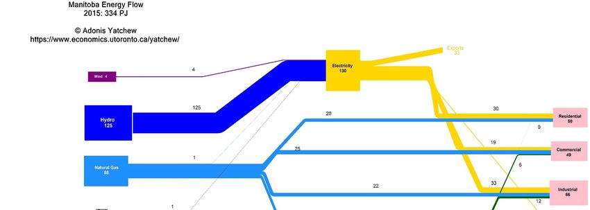
Executive Summary
Background

   1. Projected Rate Increases In May 2017, Manitoba Hydro filed a General Rate Application seeking
      rate increases of 7.9% for 2017/2018 and 2018/2019. Manitoba Hydro was granted an interim
      rate of increase of 3.36% effective August 1, 2017. In a subsequent letter, dated September 5,
      2017, Manitoba Hydro advised the Board that it projects rate increases of 7.9% for each of the
      upcoming six fiscal years followed by an increase of 4.54% in the seventh year. The cumulative
      effect would be to increase electricity rates by close to 50% in real terms over the coming
      decade.

   2. Purpose of Testimony In broad terms, the purpose of this testimony is to assess the likely
      impacts on, and responses of various customer groups to rate increases of this magnitude, as
      well as the implications for the Manitoba economy as a whole.

   3. Manitoba Resources and GDP From a resource perspective, the Province of Manitoba has the
      good fortune of being endowed with vast hydroelectric resources, very productive agricultural
      lands as well as deposits of some metals and minerals. Manitoba has a diversified economy.
      Much like most advanced economies, the dominant share of GDP – 71% – is in the service
      sector. Manufacturing comprises about 10% of GDP, construction 9%, agriculture 4%, mining
      about 2%. There is considerable variation in energy intensity and electricity intensity across the
      various sectors and sub‐sectors.

   4. Sources of Energy The dominant source of Manitoba energy (approximately 37% in 2015) is
      hydroelectricity. About 60% of energy consumed in the residential sector is electricity, the
      industrial sector electricity share is 50%, and the commercial sector share is about 40%. These
      shares are considerably higher than the corresponding Canada‐wide electricity shares which are
      42% for the residential sector, 19% for the industrial sector and 35% for the commercial sector.
      Manitoba’s reliance on electricity has been largely the result of low‐priced electricity over many
      years. It is also suggestive of the potential for substitution to other energy sources, for example
      to natural gas where it is available, in the event of large and sustained electricity price increases.

Key Energy Trends Affecting Manitoba and Manitoba Hydro

   5. Natural Gas Prices Natural gas prices are low and are likely to remain low for the foreseeable
      future. The extraction of natural gas from shale using hydraulic fracturing (‘fracking’) has
      revolutionized North American natural gas markets leading to excess supply.

           a. In the U.S., low natural gas prices have led to increased reliance on natural gas for
              generation of electricity; the cost is approximately 5 cents U.S. per kWh for high
              capacity combined‐cycle generation. This in turn has a direct impact on the
              competitiveness of Manitoba Hydro in export markets.

                                                     i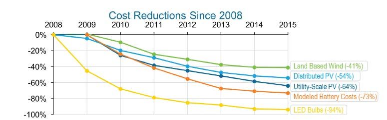
b. In Canada, low natural gas prices influence energy choices made by all classes of
              customers. The potential for substitution towards natural gas in the face of major
              electricity price increases is a significant risk for Manitoba Hydro.

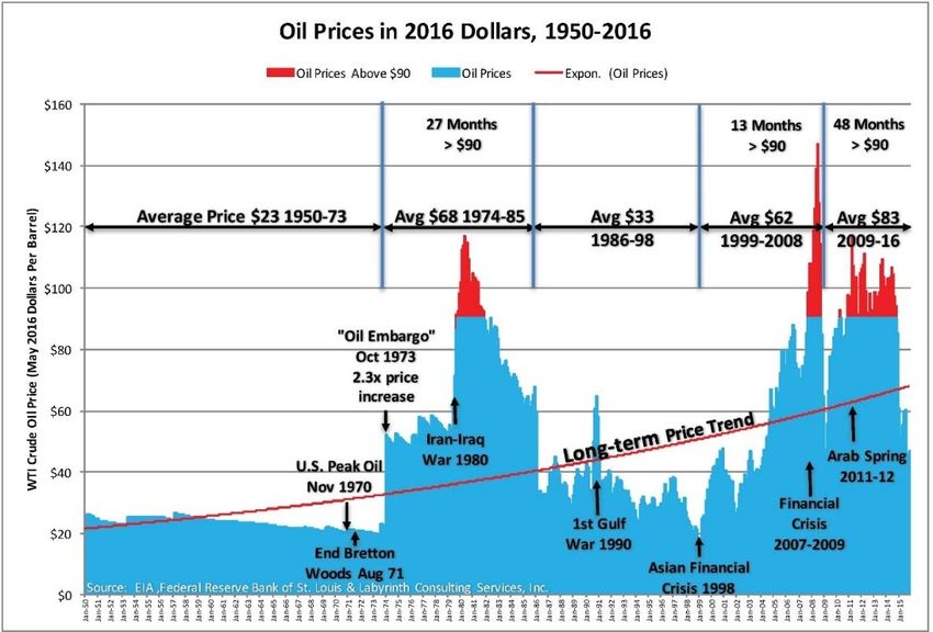
   6. Oil Prices The shale revolution has triggered profound change in world oil markets, not only
      because it has led to new sources of supply, but more importantly, because it is scalable. Shale
      oil can be brought on in tiny increments, allowing rapid response to increases in price and
      thereby reducing OPEC market power. Oil market analysts consider a return to the high oil
      prices (which exceeded $100 USD/barrel prior to 2014) unlikely. Continued low oil prices have a
      strong influence on the prosperity of Alberta and on future development of the oil sands, which
      indirectly affect the Manitoba economy.

   7. Exchange Rates Canada’s exchange rate has historically been closely linked to world oil prices.
      Exchange rates have an important effect on Manitoba’s economy as they influence demand for,
      and revenues from exports, including those in the electricity sector. Expectations about future
      oil prices inform forecasts of Canada/U.S. exchange rates.

   8. New Energy Technologies The costs of new key energy technologies have been declining
      rapidly. Since 2008, costs of wind generation have dropped by 41%; photovoltaic costs have
      dropped more than 50%; battery costs by 73%; and LED bulbs by a stunning 94%. Continuation
      of these trends could have an important impact on Manitoba Hydro domestic and export
      markets.

   9. Decentralization of Electricity Systems Electricity systems are facing powerful decentralizing
      forces, in part as a result of the scalability of new generation and storage technologies, and the
      enabling effects of information technologies. On the other hand, Manitoba Hydro, because of its
      vast hydroelectric resources, continues to operate with a highly centralized model, relying on
      massive investments in generation and transmission. These large investments have long life‐
      times, and face financial risks in a world of rapid technological innovation.

Demand Modeling and Elasticities

   10. Types of Energy Models There is a voluminous literature on the estimation of energy models of
       supply and demand. Many of the papers pertain to the electricity sector. Broadly speaking,
       three types of data can be used to infer the impacts of prices and of many other variables.

           a. Time‐Series Models By observing patterns of demand over time within a specific
              geographic area, one can infer impacts of price changes on demand, and how energy
              users adjust to such price changes. There needs to be sufficient variation in prices for
              such models to produce useful results.

           b. Cross‐Section Models By observing patterns of demand across various geographical
              areas at a single point in time, one can infer how different locations have adapted to
              varying price points, the kinds of industries that have been attracted, and the response
              of residential and commercial customers.

                                                   ii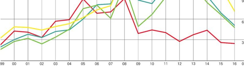
c. Panel Data Models Time‐series and cross section data can be combined into more
           comprehensive specifications which permit estimation of impacts across locations and
           through time.

    Each approach has advantages and disadvantages, and each can inform the present discussion
    of the potential impacts of large price changes on demand.

11. Types of Demand Elasticities Two classes of response measures, or ‘elasticities’ are particularly
    germane to the current discussion: the responsiveness of electricity demand to changes in the
    price of electricity (the ‘own‐price’ elasticity, or usually just the price elasticity of demand); and,
    the responsiveness of electricity demand to changes in economic activity, which in this case is
    Provincial GDP (the GDP elasticity).

        a. The price elasticity can be further refined to be sector specific, i.e., separate values may
           be estimated for the residential, commercial and industrial sectors.

        b. There is also a distinction between short‐term (say one‐year) and long‐term elasticities.
           Energy use is determined to a large degree by capital goods which take time to replace.
           Thus, short‐run responses are usually much more attenuated than longer‐term ones.

        c. A separate critical objective of energy modeling is the identification of trends which are
           evolving over time, in particular energy intensity and electricity intensity trends.

12. Estimates of Demand Elasticities The vast demand modeling literature produces a very broad
    range of electricity demand elasticities. So‐called meta‐analyses seek to aggregate and distill the
    results from many papers into single estimates. Defensible, empirically based values which are
    relevant for the present Manitoba environment are presented below:

        a. a short‐term price elasticity of ‐0.1 across all sectors; that is, an electricity price increase
           of 10% leads to a 1% decline in electricity demand in the short‐term;

        b. a long‐term overall price elasticity of ‐0.4; that is, an electricity price increase of 10%
           leads to a 4% decline in electricity demand in the long‐term;

        c. long‐term price elasticities of ‐0.35 for the residential and commercial sectors, and ‐0.5
           for the industrial sector;

        d. a GDP elasticity of 0.8; that is, an increase in GDP of 10% eventually leads to an increase
           in electricity consumption of 8%.

    Recent analyses suggest that long‐term price elasticities are roughly three times short‐term
    elasticities. Thus, impacts of price increases within the test period will not be fully realized for
    some time to come.

    While elasticities proposed by Manitoba Hydro are not unreasonable, especially given the
    degree of uncertainty associated with estimation of demand parameters, those recommended
    above are better supported by the literature.

                                                  iii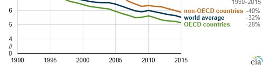
13. Stagnant Electricity Demand These recommended elasticities suggest that basic load
       (unadjusted for certain demand management activities) is likely to be stagnant over the coming
       decade. Suppose that cumulative increases in electricity prices are about 50% and that the
       economy grows at 2% per year, so that GDP is 22% larger ten years hence. Then the price
       increase reduces electricity demand by about 20% (‐0.4 x 50%) and GDP growth increases
       demand by about 18% (.8 x 22%).

   14. Business Cycle Risks The current economic expansion is in its ninth year, so that a recession may
       not be far off. This will have an adverse effect on electricity demand.

   15. Declining Energy Intensity Over the last 25 years, energy intensity, that is the amount of energy
       used per dollar of GDP, has been falling by more than 1% per year in Canada, a figure
       comparable to the average for OECD countries. Manitoba energy intensity has been dropping
       more rapidly, at a rate closer to 2% per year.

   16. Electricity Intensity Patterns of electricity intensity in Manitoba have been mixed. In the service
       sector, which is by far the largest, intensity dropped by about 25% between 2005 and 2012, but
       by 2015 it had recovered to 2005 levels. Intensity in the manufacturing sector peaked in 2005,
       and has been displaying a fairly steady decline since that time. Agricultural sector intensity
       remained high until 2005, but subsequently dropped significantly.

   17. Energy Poverty Manitoba has a relatively low rate of energy poverty in comparison to some
       other provinces: about 7% of households spend 10% or more of their income on energy.
       However, the incidence of energy poverty varies significantly across the Province and is
       particularly high in remote communities where prices of many goods, among them energy, are
       high. The projected growth in electricity prices will increase rates of energy poverty.

   18. First Nations The impact on energy poverty, which is already high in remote and First Nations
       communities, is likely to be especially acute given the limited possibilities for energy
       substitution. In addition, low incomes will hamper substitution of capital goods, such as
       improved insulation, and efficient windows and doors. Commercial and industrial
       establishments will also be adversely affected, particularly in the absence of energy substitutes
       such as natural gas.

Macroeconomic Issues

   19. Energy Price Shocks Market economies have experienced major energy price shocks. Past
       experiences are helpful in bounding the likely effects of significant electricity price increases in
       Manitoba. The dramatic oil price shocks of the 1970s which were largely unanticipated, led to
       economic contractions of half a per cent or less. The cumulative impact on U.S. GDP of the oil
       price shock in the late 1970s is estimated to be about 3%.

   20. Risks Associated With Exchange Rates and Commodity Prices Certain sectors of the Manitoba
       economy are subject to large, difficult‐to‐predict variations in key variables. Exporters are
       subject to exchange rate variations: over the last decade, the Canadian dollar has varied from
       below 70 cents/USD to well above parity. Wheat prices, which reached a post‐recession high of

                                                     iv
$9 US/bushel in 2012, have since declined to $4 ‐ $5 US/bushel in 2017. Nickel, copper, zinc and
        gold prices have also exhibited large swings.

    21. Vulnerable Economic Sectors Electricity prices affect all households, firms, institutions and
        agencies. The extent of response depends on the electricity intensity and alternatives available.

             a. In the manufacturing sector, the most vulnerable industries appear to be ‘basic
                chemicals’ and ‘pulp and paper’ where electricity comprises high shares of costs. Iron
                and steel mills, foundries and non‐ferrous metal production also have significant
                electricity cost shares.

             b. In the agricultural sector, ‘greenhouses’ and ‘animal production’ have significant
                electricity cost shares.

             c. In the mining sector, ‘support activities for oil and gas production’ and extraction of
                metals also have significant electricity cost shares.

        Where natural gas is available, some of these industries may engage in fuel substitution. Others
        are likely to carefully consider, or reconsider future investment plans.

    22. Macroeconomic Impacts of Large Electricity Price Increases In the event that large electricity
        price increases are approved over the coming years, the Manitoba economy will adapt.1

             a. The net effect on GDP may eventually be modest, but in the interim, there are likely to
                be significant adjustment costs.

             b. In some locations, particularly those which are heavily dependent on an industry that is
                sensitive to electricity prices, there could be large local impacts on employment,
                incomes and output.

             c. The projected rate increases are not of the same magnitude as the energy price shocks
                of the 1970s. However, given that in the short‐term, demand for electricity is highly
                price‐inelastic, the steepness of the projected rate increases will impose a significant
                burden, particularly on households, businesses and institutions that do not have access
                to substitutes, such as natural gas.

Concluding Observations

    23. Regulatory Signaling The regulatory decision made in this proceeding, which ostensibly deals
        with rate increases over a two‐year test period, will have an important impact on decision
        making by industry because it will signal the likely future path of rate increases. Approval of

1
 Ontario has experienced electricity price increases in excess of 50% since 2009. Notwithstanding these increases,
and the fluctuations in exchange rates, the Ontario economy continued to grow and the manufacturing share
remained steady at about 13% of Provincial GDP.

                                                        v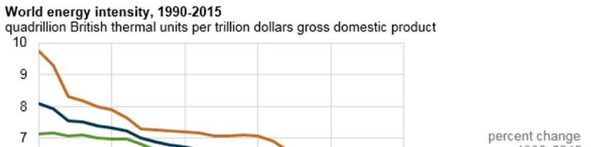
increases that are close to the proposed 7.9% will suggest the acceptance of Manitoba Hydro
           arguments, and its focus on the time profile of future financial ratios.

       24. Excess Capacity Large increases will induce a price response, which in a period of excess
           capacity may be sub‐optimal as it will erode revenues at a time when marginal costs of
           production are low.

       25. Cost Reductions Manitoba Hydro operates under a ‘cost‐of‐service’ regulatory regime. (Many
           other jurisdictions have moved to a mode of incentive regulation in order to improve incentives
           for cost minimization.) Manitoba Hydro is implementing a “Workforce Reduction Plan” which
           would eliminate 900 positions (15% of the workforce) over the course of two to three years.2

       26. Intergenerational Fairness One might ask whether the projected rate increases are equitable
           from an intergenerational standpoint.

                a. Expansion of hydroelectric systems, such as that in Manitoba, involves lumpy
                   investments in generation (to exploit scale economies) and transmission (as supply
                   sources are distant from load). They do not enjoy the beneficial scalability features of
                   solar, wind and natural gas generation.3

                b. This leads to long‐term cyclical pressures on rates. Current customers have benefited
                   from past investments, particularly those that have been largely depreciated, but
                   remain functional. Future customers will need to pay for current projects. The calculus
                   of intergenerational fairness is therefore, at a minimum, complex, and may not lead to
                   unequivocal answers.

                c. Rate‐smoothing is a useful tool for promoting inter‐generational equity. The projected
                   profile is more in the nature of a step function over six years, followed by a rapid decline
                   to increases close to the rate of inflation. A ramped sequence of increases, perhaps
                   linked to a clear demonstration of efficiencies achieved by Manitoba Hydro, may
                   provide a useful framework for promoting internal efficiencies, allowing time to adjust
                   to electricity rates, and distributing costs more equitably over each generation of
                   consumers.

       27. Mitigation of Rate Increases The effects of the large projected increases, should they be
           approved, could in theory, be mitigated.

                a. Special industrial rates could be offered to those firms with large electricity cost shares.
                   But this would be viewed as inequitable by other customers.4 Alternatively, the
                   Government might implement incentives to retain major industrial customers.

2
 Manitoba Hydro, 2017/18 & 2018/19 General Rate Application, Integrated Financial Forecast, May 12, 2017, Tab
3, page 10 of 22.

3
    Or for that matter, shale oil extraction.

4
 Though rate design has inherent ambiguities. When there are significant common costs, there is no unique cost
allocation based on the principle of cost causality.

                                                        vi
b. There would be a substantial increase in the number of households facing energy
          poverty, however it is measured. To alleviate this effect will require funds either from
          other Manitoba Hydro customers, or from Government coffers.

28. The Current U.S. Administration In any discussion of Canada’s economic circumstances,
    consideration of the effects of the current U.S. administration cannot be ignored. The North
    American Free Trade Agreement is being re‐negotiated at the initiative of the U.S. At a
    minimum, this injects considerable uncertainty into trade relations with our largest trading
    partner. The U.S. administration has also altered direction on its decarbonization policies,
    disengaging from the Paris Agreement and making efforts to revive the coal industry. Together,
    these factors are likely to have a dampening effect on investment, and weaken prospects for
    long‐term power sales agreements that are premised on clean hydro‐electric power.

                                              vii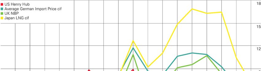
Contents
A.      Introduction .......................................................................................................................................... 1
B.      Background ........................................................................................................................................... 2
     B.1 Economic Setting ................................................................................................................................ 2
     B.2 The Manitoba Energy Sector .............................................................................................................. 4
     B.3 Oil and Natural Gas Markets ............................................................................................................... 8
     B.4 Costs of Key Technologies Have Been Dropping Dramatically ......................................................... 12
     B.5 Decentralization of Electricity Systems............................................................................................. 13
     B.6 Regulatory Considerations ................................................................................................................ 17
C.      Demand Modeling .............................................................................................................................. 21
     C.1 Energy Demand Modeling ................................................................................................................ 21
     C.2 Price Elasticities................................................................................................................................. 25
     C.3 GDP Elasticities, and Energy and Electricity Intensities. ................................................................... 28
D.      Manitoba Hydro Electricity Prices....................................................................................................... 32
     D.1 Rates, Costs and Intergenerational Equity ....................................................................................... 32
     D.2 Bill Affordability and Energy Poverty ................................................................................................ 35
E.      Macroeconomic Impacts of Electricity Price Increases....................................................................... 42
     E.1 Energy Price Shocks........................................................................................................................... 42
     E.2 Exchange Rates ................................................................................................................................. 45
     E.3 Commodity Prices ............................................................................................................................. 48
     E.4 Electricity Intensity Varies Widely Across Some Sectors of the Manitoba Economy ....................... 49
F.      Concluding Observations .................................................................................................................... 51
Appendix 1: Scope of Work and Summary Responses .............................................................................. 54
Appendix 2: Curriculum Vitae – Adonis Yatchew....................................................................................... 61
Appendix 3: References on Elasticities ....................................................................................................... 71
Appendix 4: Manitoba Electricity Cost Shares by Sub‐Sector .................................................................... 77

                                                                              viii
1 A. Introduction
2
3 1. In May 2017, Manitoba Hydro filed a General Rate Application seeking rate increases of
4 7.9% for 2017/2018 and 2018/2019. Manitoba Hydro was granted an interim rate increase
5 of 3.36%, effective August 1, 2017.5 In a subsequent letter, dated September 5, 2017,
6 Manitoba Hydro advised the Board that it projects rate increases of 7.9% for each of the
7 upcoming six fiscal years followed by an increase of 4.54% in the seventh year.6 The
8 cumulative effect would be to increase electricity rates by close to 50% in real terms over
9 the coming decade.
10
11 2. In broad terms, the purpose of this testimony is to assess the impacts on various customer
12 groups and their likely responses; and to provide an analysis of the likely macroeconomic
13 consequences of electricity price increases. We begin by situating the discussion within
14 the context of Manitoba’s economy, its patterns of energy and electricity use, critical
15 trends related to energy, and the regulatory environment. In order to assess customer
16 responses, we draw upon the large literature of energy modeling and in particular the
17 estimation of price and income elasticities. Consideration is given to the incidence of
18 energy poverty and the impacts on remote and First Nations communities. Subsequent
19 sections discuss the likely macroeconomic effects of the projected rate increases.
20
21 3. In the concluding section, comments are provided relating the projected price increase to
22 Manitoba’s decarbonization agenda.
23
5
PUB Order 80/17, July 31, 2017, available at http://www.pubmanitoba.ca/v1/proceedings‐
decisions/orders/pubs/2017%20orders/80‐17.pdf.
6
Manitoba Hydro letter to the PUB, available at
https://www.hydro.mb.ca/regulatory_affairs/pdf/electric/general_rate_application_2017/00.0000001_cover_lett
er_dated_september_5.pdf.
11 B. Background
2 B.1 Economic Setting7
3 4. Manitoba has a population of approximately 1.3 million. Its 2016 GDP was $67 billion with
4 per capita output of $51,500. In part as a response to declines in commodity prices,
5 Manitoba economic growth slowed during the 2014‐2016 period, but is expected to have
6 improved for the 2017 year. As a result of its industrial diversity, inter‐provincial and
7 international exports, high labour force participation and low per‐capita debt, Manitoba’s
8 economic growth has been strong in comparison to a number of other provinces.
9
10 5. Manitoba is endowed with excellent fresh water and hydraulic resources, very productive
11 agricultural lands, and a variety of deposits of metals and minerals. Its economy is well
12 diversified. There is considerable variation in energy and electricity intensity across sub‐
13 sectors, making some firms more vulnerable to electricity price increases, while others
14 more resilient to such price changes.
15
16 Figure 1: Manitoba GDP Shares 20168
Utilities Mining
Agriculture4% 2%
4%
Construction
9%
Manufacturing
10%
Services
71%
17
7
See Manitoba Provincial Budget & Supporting Documents, available at
http://www.manitoba.ca/budget2017/index.html and Manitoba Economic Highlights,
https://www.gov.mb.ca/finance/pubs/highlights.pdf .
8
Source: Statistics Canada, Table 379‐0028 Gross domestic product (GDP) at basic prices.
21 6. Much like most advanced economies, the largest portion of Manitoba GDP ‐‐ 71% ‐‐ is in
2 services. This sector comprises a virtually identical portion of Canada‐wide GDP. (See
3 Figures 1 and 2.) Major sub‐sectors include real estate and rental and leasing (12%),
4 wholesale and retail trade (11%), health care and social assistance (9%), public
5 administration (8%), transportation and warehousing (6%), finance and insurance (6%),
6 and educational services (5%).
7
8 Figure 2: Canada GDP Shares 20169
9
Utilities Mining
2% 8%
Agriculture
2%
Construction
7%
Manufacturing
10%
Services
71%
10
11
12
13
14 7. Manufacturing comprises about 10% of Manitoba GDP. This sector consists of food
15 processing, manufacture of transportation equipment (aerospace and motor vehicle),
16 agricultural implements, chemicals (pharmaceutical and agricultural), metal and wood
17 products and electrical equipment. Most manufactured goods are sold in other provinces
18 or exported to the U.S. Export demand is sensitive to both exchange rates and economic
19 activity in recipient countries.
20
21
9
Source: Statistics Canada, Table 379‐0031 Gross domestic product (GDP) at basic prices.
31 8. Exchange rates have an important effect on Manitoba’s economy as they affect demand
2 for, and revenues from exports, including those in the electricity sector. Canada’s
3 exchange rate has historically been closely linked to world oil prices, as we will discuss
4 further below. Expectations about future oil prices inform forecast exchange rates.
5
6 9. In any discussion of Canada’s economic circumstances, consideration of the effects of the
7 current U.S. administration cannot be ignored. The North American Free Trade
8 Agreement is being re‐negotiated at the initiative of the U.S. At a minimum, this injects
9 considerable uncertainty into trade relations with our largest trading partner. The U.S.
10 administration has also altered direction on its decarbonization policies, disengaging from
11 the Paris Agreement and making efforts to revive the coal industry.10 Together, these
12 factors are likely to dampen the Manitoba investment climate in the manufacturing
13 sector, and weaken prospects for long‐term power sales agreements that are premised on
14 clean hydro‐electric power.
15
16 B.2 The Manitoba Energy Sector
17
18 10. A particularly informative visual representation of energy sources and uses is provided by
19 ‘Energy Flow’ diagrams, also known as Sankey diagrams. Figure 3 depicts this type of
20 diagram for the Province of Manitoba. ‘Pipe’ diameters reflect the magnitudes of flows. 11
10
Notwithstanding these developments, the U.S. Government released a major report confirming the
anthropogenic nature of climate change. See “Climate Science Special Report”, Fall 2017, available at
https://science2017.globalchange.gov/chapter/front‐matter‐about/.
11
Such diagrams have been in existence since the 1800s. They are widely used to depict energy flows, for example
Lawrence Livermore National Laboratories (LLNL) produce such diagrams for all U.S. states, see https://flowcharts.llnl.gov/.
LLNL also produces U.S. national carbon flow diagrams. The International Energy Agency produces Sankey diagrams at
national and continental levels http://www.iea.org/Sankey/index.html#?c=World&s=Balance.
Figure 3 was produced using e!Sankey software, https://www.ifu.com/e‐sankey/ based on CANSIM data.
For further discussion of uses of Sankey diagrams, see Economist, “Data Visualisation, Sankey or Harness?” July 4th,2011;
A. Yatchew, “Economics of Energy: Big Ideas for the Non‐Economist”, Energy Research and Social Science, 1(1), 2014, pages
74‐78; “Using Sankey diagrams to map energy flow from primary fuel to end use”, Veena Subramanyam, Deepak
Paramshivan, Amit Kumar, Md. Alam Hossain Mondal, Energy Conversion and Management, 91, 2015, pages 342–352; and
A. Yatchew 2016: “Rational vs ‘Feel‐Good’ Carbon Policy”, Energy Regulation Quarterly, Vol. 4, Issue 3,
41 11. At the top left is the total ‘primary’ energy of all types which in 2015, the latest year for
2 which comprehensive data are available, was 334 peta joules (PJ). The total is obtained by
3 summing the values of the five primary sources of energy on the left (wind, hydro, natural
4 gas, coal and petroleum).
5
6 12. The left side of the diagram represents the supply side, while the pink boxes on the right
7 represent the demand side.
8
9 13. The largest source of energy in Manitoba is hydraulic, which comprises about 125 PJ, or
10 37% of total energy. Almost all electricity produced in Manitoba comes from hydraulic
11 sources. The second largest source of energy is petroleum at 116 PJ, or 35% of provincial
12 energy, the vast majority of which is used in the transportation sector. The third largest
13 energy source is natural gas at 88 PJ or 26% of total energy.
14
15 14. Next consider the demand side, which is comprised of residential, commercial, industrial
16 and transportation sectors.12 Manitoba’s successful development of cheap and accessible
17 hydraulic electricity is reflected in its share of total energy, and its shares within each end‐
18 use sector.
19
20 a. About 60% (30 PJ of 50 PJ) of energy used in the residential sector is
21 electricity.
22 b. For the industrial sector the share is 50% (33 PJ of 66 PJ).
23 c. For the commercial sector the share is 39% (19 PJ of 49 PJ).
24
25 In short, Manitoba is an electricity intensive province where hydraulic energy represents the
26 largest energy source. This is a price phenomenon, thanks to abundant hydraulic sources.13
http://www.energyregulationquarterly.ca/articles/ rational‐vs‐feel‐good‐carbon‐policy‐transferability‐subsidiarity‐and‐
separation#sthash.GBtFuIOG.dpbs.
12
There is also a non‐energy sector which corresponds primarily to petrochemical feedstocks.
13
A comparison with Canada‐wide numbers illustrates the point. Natural gas is the dominant fuel in the
residential, commercial and particularly the industrial sector where more than 50% of energy comes directly from
this source (as well as a portion that comes indirectly through gas‐fired electricity generation). See Canada‐wide
Sankey diagrams available at https://www.economics.utoronto.ca/yatchew/.
51 15. The Sankey diagram depicting energy flows in Manitoba (Figure 3) also provides a
2 departure point for considering the impacts of changes in the price of electricity. Where
3 natural gas is available, substantial increases in electricity prices could lead to substitution
4 to gas in the residential, commercial and industrial sectors, particularly given the relatively
5 low shares of natural gas there.
6
7 16. There is great potential for increased electricity consumption in the transportation sector,
8 but a dramatic shift awaits further large drops in the costs and range of future generations
9 of electric vehicles. In Manitoba, such a shift would contribute greatly to the
10 decarbonization agenda as Manitoba has large supplies of clean hydraulic sources for the
11 foreseeable future.
12
13 17. The energy in each sector either produces ‘energy services’ or is lost, usually in the form
14 of heat. The least ‘efficient’ sector is transportation where 75%‐80% of energy is
15 ‘rejected’. Depending on the source of energy and the types of uses, efficiency in the
16 residential, commercial and industrial sectors ranges from 50% to 80%. While it might
17 appear that we are very inefficient, ‘wasting’ well over half of the energy we produce, this
18 is primarily a reflection of the state of technology and the second law of thermodynamics
19 which states that whenever energy is transformed from one form to another, a portion is
20 lost.14
21
22 18. The Sankey diagram is also useful for informing decarbonization discussions. Manitoba is
23 very well positioned with such a large share of hydraulic source energy. Its use of coal is
24 minimal and the remainder of non‐transportation energy comes from natural gas, the
25 hydrocarbon with the lowest carbon footprint (roughly half that of coal). The dominant
26 share of energy‐related carbon generated in Manitoba is in the transportation sector,
27 which is the most difficult to decarbonize.
28
14
Estimates produced by Lawrence Livermore National Laboratories suggest that roughly two‐thirds of energy in
the U.S. is ‘rejected’ and only one third produces energy services. See
https://flowcharts.llnl.gov/content/assets/images/energy/us/Energy_US_2016.png.
61 Figure 3: Manitoba Energy Flow (Sankey Diagram)
2
71 B.3 Oil and Natural Gas Markets
2
3 19. An understanding of oil and natural gas markets and scenarios of their future price paths
4 is important to the current analysis in several ways.
5
6 a. First, natural gas competes with electricity in certain industrial, commercial
7 and residential applications, particularly if the end‐use is space heating or
8 process heat. A large increase in electricity prices could lead to loss of
9 electricity load to natural gas.
10
11 b. Second, low‐priced natural gas is the ‘go‐to’ fuel for electricity generation in
12 many parts of North America, including states neighboring Manitoba, and the
13 MISO transmission system to which Manitoba belongs.15 This in turn affects
14 Manitoba Hydro export markets.
15
16 c. Third, oil prices have an important impact on Canadian export revenues and
17 on exchange rates. The precipitous decline in oil prices which began in mid‐
18 2014 has had a dramatic impact on the economy of Alberta and to a lesser
19 degree on Saskatchewan and Manitoba. Canada has vast reserves of oil,
20 mainly in the form of bitumen. But these reserves are among the highest
21 priced in the world.
22
23
24 20. What is the outlook for natural gas prices? A decade ago, it was widely believed that the
25 U.S. would need to begin importing natural gas. Liquid natural gas (LNG) terminals were
26 planned and some were built.16 Then came the shale revolution. By efficiently combining
15
Low natural gas prices have led to a significant shift away from coal‐fired electricity generation in the U.S.
towards natural gas generation. Roughly comparable amounts of electricity are generated from each of these two
sources in the U.S.
16
LNG shipping requires liquefaction terminals at the exporting site, and re‐gasification at the importing site.
Initially, the U.S. began to build re‐gasification terminals. These sites have been largely converted to liquefaction.
Qatar is the largest LNG exporter, followed by Australia. Floating storage and re‐gasification carriers can serve as
LNG importing terminals.
81 two technologies – horizontal drilling and hydraulic fracturing (fracking) – cost‐effective
2 North American gas reserves grew very rapidly.
3
4 Figure 4: Gas prices
5 USD/mmBtu
6
7 BP Statistical Review of World Energy 2017 © BP p.l.c. 2017
8
9 21. Natural gas prices worldwide dropped dramatically in 2009, as a result of the financial
10 crisis. However, by 2012 they had recovered except in North America (Figure 4).17 What
11 we observed were the consequences of shale revolution. This in turn led to a
12 reconfiguration of natural gas flows across North America as major natural gas supplies
13 were developed, for example, in Texas and Pennsylvania, reducing the need for Canadian
14 natural gas and leading to reduced use of the TransCanada Mainline.
15
16 22. In the past, natural gas markets have been continental (hence the separate benchmark
17 prices in Figure 4). But recently, there has been a gradual globalization as LNG becomes
17
LNG prices in Japan sky‐rocketed in 2011 as a result of the Fukushima meltdown.
91 increasingly competitive in overseas markets. By 2015 about 40% of total natural gas
2 trade moved by sea, and prices in distant markets began to converge.18
3
4 23. While globalization increases the demand for North American natural gas, there is little
5 evidence to suggest that a dramatic price increase is likely; natural gas will continue to
6 provide strong competition to electricity.
7
8 24. Though largely unanticipated, the revolution in natural gas would eventually lead to
9 perhaps the most dramatic change in oil markets since the 1970s OPEC price increases.19,20
10 One might think that the main effect of the fracking revolution on oil prices is through the
11 increase in recoverable supplies. However, the peculiar features of the shale revolution
12 have altered the nature of oil markets in another critical way. For the first time, additional
13 oil can be brought online in tiny increments – the cost of a productive shale well is three
14 orders of magnitude smaller than Arctic or deep‐sea projects.
15
16 25. The scalability of shale has fundamentally altered the strategic behavior of OPEC.
17 Whereas in the past OPEC might have coordinated a supply reduction to sustain prices, it
18 is far more limited now in its ability to do so because shale producers (and others) can fill
19 the gap. Shale has provided for a scalable response by many producers as market
20 conditions change. This feature further limits unilateral or cartelized market power.
18
“Long Promised, the Global Market for Natural Gas Has Finally Arrived”, Russell Gold and Alison Sider, Wall
Street Journal, June 6, 2017. See also MIT Energy Initiative, The Future of Natural Gas, Cambridge: June 2011.
19
Though in 2012, Berkeley physics Professor Richard Muller writes “Shale oil production could truly be a
disruptive technology, with a large and positive impact on the US balance of trade, severe repercussions for the
OPEC oil cartel, and a serious challenge to alternative‐transportation technologies, particularly natural gas and
synfuel. Shale oil could turn conventional oil into the new whale oil, replaced by a far more abundant source.”
Richard A. Muller, Energy for Future Presidents: The Science Behind the Headlines, 2012, (Kindle Locations 1679‐
1682). W. W. Norton & Company. Kindle Edition. In that same book, Muller sees $60 USD / barrel as a long‐term
limit price for oil. At the time of his writing, the world price of oil was well over $100 USD / barrel.
20
The historic paths of oil and (North American) natural gas prices display a surprising degree of correlation. In
fact, some have argued that the drop in world oil prices beginning in 2014 was signaled by the decline in North
American natural gas prices which began in 2008. See, e.g., Dimitri Dimitropoulos, and Adonis Yatchew 2017,
“Discerning Trends in Commodity Prices”, Macroeconomic Dynamics, doi:10.1017/S1365100516000511.
101 Scalability of shale also reduces risks – wells do not last long, but capital requirements are
2 low and lead‐times short.
3
4 26. Not long ago, ‘peak oil’ meant that one day, in the not too distant future, we would reach
5 peak production as supplies ran out. Now ‘peak oil’ refers to the day when demand levels
6 off and begins to fall. Technological innovations to a post‐carbon world are leading the
7 way. Shale, bitumen and undersea resources are unlikely to run out, and the key question
8 is what fraction of proven reserves will not be extracted. This in turn creates incentives for
9 those with large cheap reserves (such as Saudi Arabia) to sell more today rather than
10 saving reserves for an uncertain future.21
11
12 27. In the absence of innovation in electric vehicles which would lead to their wide spread
13 adoption in growing economies such as China and India, demand for oil should continue to
14 grow for a time. The question is when we will reach the tipping point in the sector that is
15 the most difficult to decarbonize – transportation.
16
17 28. To summarize, low natural gas prices exert competitive pressures on Manitoba Hydro in
18 domestic markets to the extent that they provide a viable alternative to electricity, and in
19 export markets because they drive down electricity prices there. Low oil prices put
20 downward pressure on the exchange rate, which enhances export competitiveness of
21 Manitoba industries and improves Canadian dollar revenues of Manitoba Hydro electricity
22 sales.
23
21
See, for example, “Get Ready for Peak Oil Demand. There’s a growing consensus that the end of ever‐rising
consumption is in sight. The big question that many oil companies are debating: When?”, Lynn Cook and Elena
Cherney, Wall Street Journal, May 26, 2017.
111 B.4 Costs of Key Technologies Have Been Dropping Dramatically
2
3 29. The costs of emerging technologies which are transforming electricity industries have
4 been dropping at a rapid pace. Since 2008, costs of wind generation have dropped by
5 41%; photovoltaics have dropped more than 50%; battery costs by 73%; and LED bulbs by
6 a stunning 94%. (See Figure 5 below.)
7
8 Figure 5 – Cost Reductions in Key Technologies22
9
10
11 30. Non‐dispatchable generation such as on‐shore wind is priced at about 5 U.S. cents/kWh
12 for new installations at a capacity factor of 39%. Solar photo‐voltaic is at 7 U.S. cents/kWh
13 at a capacity factor of 26%. Combined cycle natural gas electricity generation for new
14 installations costs about 5 U.S. cents/kWh if used at high capacity (87%), and conventional
15 combustion turbine generation is at about 9 U.S. cents/kWh if used at low capacity
16 (30%).23
22
Source: “Revolution … Now, The Future Arrives for Five Clean Energy Technologies – 2016 Update”, U.S.
Department of Energy, September 2016. Available at https://www.energy.gov/eere/downloads/revolutionnow‐
2016‐update. “Notes: Land based wind costs are derived from levelized cost of energy from representative wind
sites… Distributed PV cost is average residential installed cost... Utility‐Scale PV cost is the median installed cost…
Modeled battery costs are at high‐volume production of battery systems, derived from DOE/UIS Advanced Battery
Consortium PHEV Battery development projects. LED bulb costs are cost per lumen for A‐type bulbs...”
23
These are Levelized Cost of Energy (LCOE) numbers which embed assumptions about depreciation lifetimes, cost
of fuel and, as indicated, utilization capacity factors. U.S. Energy Information Administration April 2017 Table A1a.
Estimated LCOE (weighted average of regional values based on projected capacity additions) for new generation
resources, for plants entering service in 2019 “, available at https://www.eia.gov/outlooks/aeo/pdf/electricity_
generation.pdf. Combined heat and power systems, because of their high efficiency, have the potential for
121 B.5 Decentralization of Electricity Systems
2
3 31. Historically, the centralized structure of electricity industries has been driven by three
4 critical features. First, non‐storability of electricity meant that supply and demand needed
5 to be balanced virtually instantaneously. Second, scale economies in generation led to
6 electricity being produced at a relatively small number of locations. Third, the essentiality
7 of electricity to every‐day life underscored the need for a very high degree of reliability.
8
9 32. Scale economies in electricity generation increased into the 1970’s, at which time they
10 began to level off. Minimum efficient scale declined. Electricity networks, both
11 transmission and distribution, which would transport and distribute electrons, were and
12 continue to be natural monopolies, but at different spatial scales.24
13
14 33. In many jurisdictions, as a result of scale economies, (and some have argued due to
15 vertical economies of scope), the electricity industry was vertically integrated, as is the
16 case in Manitoba. In other jurisdictions, the distribution segment of the industry was
17 serviced by a number of distributors.
18
19 34. By the late 20th century, the centripetal forces which centralized electricity industry
20 structure began to weaken. The generation segment in many instances was no longer
21 seen as a natural monopoly.25 In various jurisdictions, the separation of natural monopoly
22 components (i.e., transmission and distribution) from potentially competitive segments
23 (i.e., generation and energy services) took place. This ‘unbundling’ was intended to lead
increasing market penetration. See Combined Heat and Power Technical Potential in the United States, U.S.
Department of Energy, March 2016, available at
https://www.energy.gov/sites/prod/files/2016/04/f30/CHP%20Technical%20Potential%20Study%203‐31‐
2016%20Final.pdf; also Many industries use combined heat and power to improve energy efficiency, U.S. Energy
Information Administration, July 27, 2016, available at https://www.eia.gov/todayinenergy/detail.php?id=27252.
24
The power grid was named the greatest engineering achievement of the 20th century by the U.S. National
Academy of Engineering. The main selection criterion was “how much an achievement improved people’s quality
of life”. See “Great Achievements and Grand Challenges”, The Bridge, September 1, 2000 Volume 30 Issue 3 and 4,
pages 5‐10.
25
Previously, efficient scale for coal‐fired and nuclear units was on the order of 1000 MW. The size of hydro‐
electric units depended critically on siting.
131 to increased competition, primarily in generation. In a few jurisdictions, industries were
2 restructured and competitive forces were introduced, with varying degrees of success.
3
4 35. Still, the need for coordination, reliability and the natural monopoly characteristics of the
5 grid, continued to be the fundamental centralizing drivers of the structure of the industry.
6
7 36. Transformation of electricity industries began gradually in the first decade of the 21st
8 century. The information revolution had spawned new technologies, often called ‘smart’
9 technologies, which would improve responsiveness of the grid, facilitate more rapid
10 identification and correction of faults, and eventually enable demand side response to grid
11 or market conditions.
12
13 37. At the same time, the decarbonization agenda, which was being pursued most
14 aggressively in Europe, began to drive innovation in renewables. Feed‐in‐tariffs and other
15 stimuli were producing rapid cost declines and efficiency improvements in renewable
16 technologies, particularly in solar and wind generation.26 While one tends to associate
17 successful implementation of solar technology with sun‐lit locations and relatively little
18 precipitation, grid parity is being achieved in some countries that are not endowed with
19 either of these traits.27
20
21 38. Because solar and wind generation are non‐dispatchable, i.e., intermittent, the value to
22 the system is not fully reflected by the costs of production. Backup generation (usually
23 natural gas) or electricity storage is required to ensure that sufficient electricity is
24 available when needed.
26
Between 2010 and 2016, average prices resulting from auctions have declined from about $90 USD/MWh to
below $50 USD/MWh for wind generation. For solar, the decline for the same period has been from $250
USD/MWh to about $50 USD/MWh, a precipitous drop. See Renewable Energy Auctions. Analysing 2016,
International Renewable Energy Agency, 2017, page 16, Figure 2.1, available at
http://www.irena.org/DocumentDownloads/Publications/IRENA_Renewable_Energy_Auctions_2017.pdf.
27
A 10 MW solar farm in the UK has recently been built without government subsidy. See “Solar Power
Breakthrough as Subsidy Free Farm Open”, by Nathalie Thomas, Financial Times, September 25, 2017, accessed at
https://www.ft.com/content/8ea432e4‐a1e9‐11e7‐9e4f‐7f5e6a7c98a2. Note that this facility is two orders of
magnitude smaller than conventional coal‐fired stations of 1000 MW.
141 39. Storage technologies have also been experiencing major cost reductions, but have not yet
2 reached a tipping point. Though, in some instances, solar‐cum‐battery installations have
3 achieved unexpectedly low costs.28
4
5 40. Solar is extremely scalable (think solar powered calculators and parking meters) though
6 larger facilities enjoy a significant cost advantage over small scale roof‐top installations.
7
8 41. Scalability and storage, supported by innovative uses of information technologies, are
9 combining to disrupt the conventional utility model. And that model is more susceptible
10 to disruption if the price of electricity is relatively high. Residential and commercial
11 customers are then more likely to invest in on‐site solar to reduce their overall electricity
12 costs.
13
14 42. Self‐generation and ‘net‐metering’ is posing a serious challenge to the conventional
15 electricity utility model. In some jurisdictions this has led to a confrontation between
16 utilities and their owners, and companies selling and installing distributed solar
17 generation, and their customers.29
18
19
28
In January 2017, a Hawaii electricity cooperative signed an agreement paying $110 USD / MWh for dispatchable
electricity from a combined solar and battery storage system. See “Hawaii co‐op signs deal for solar+storage
project at 11¢/kWh”, by Gavin Bade, UtilityDive, January 10 2017, accessed at
http://www.utilitydive.com/news/hawaii‐co‐op‐signs‐deal‐for‐solarstorage‐project‐at‐11kwh/433744/ . A few
months later, Tucson Electric signed a similar deal but at a much lower price. See “Updated: Tucson Electric signs
solar + storage PPA for 'less than 4.5¢/kWh'”, by Gavin Bade, UtilityDive, May 23, 2017, accessed at
http://www.utilitydive.com/news/updated‐tucson‐electric‐signs‐solar‐storage‐ppa‐for‐less‐than‐45kwh/443293/ .
29
Perhaps the most prominent clash has been between Warren Buffet, whose Berkshire Hathaway owns NV
Energy, a Nevada electricity utility, and Elon Musk, whose SolarCity company installs solar panels. See “In a clash
of titans, Warren Buffett beat Elon Musk in Nevada”, Nick Cunningham, Business Insider, December 30, 2015,
http://www.businessinsider.com/warren‐buffett‐beat‐elon‐musk‐on‐solar‐in‐nevada‐2015‐
12?pundits_only=0&get_all_comments=1&no_reply_filter=1; “Warren Buffett controls Nevada’s legacy utility.
Elon Musk is behind the solar company that’s upending the market. Let the fun begin”, Noah Buhayar, Bloomberg
Businessweek, January 28, 2016, https://www.bloomberg.com/features/2016‐solar‐power‐buffett‐vs‐musk/;
“Solar Showdown In The Nevada Desert: Warren Buffett Vs. Elon Musk?”, Michael Lynch, Forbes, February 23,
2016, https://www.forbes.com/sites/michaellynch/2016/02/23/solar‐showdown‐in‐the‐nevada‐desert‐buffett‐vs‐
musk/#5b845aed1766; “Buffett vs. Musk: The clash of old and new energy titans”, Daniel Rothberg, Las Vegas Sun,
May 2, 2016, https://lasvegassun.com/news/2016/may/02/buffett‐vs‐musk‐the‐clash‐of‐old‐and‐new‐energy‐ti/.
151 43. In a landmark study entitled Utility of the Future, a group at MIT has conducted a wide‐
2 ranging analysis of how the electricity utility business is changing, and how companies,
3 regulators and policy‐makers need to adapt.30 That study argues that fundamental
4 changes are underway in the supply and consumption of electricity. Among the major
5 factors driving the change are “emerging distributed technologies ‐‐ including flexible
6 demand, distributed generation, energy storage, and advanced power electronics and
7 control devices”. Rapidly decreasing costs in information technologies are enabling
8 synchronization of various energy supply, demand and storage resources.
9
10 44. The MIT study identifies a series of core findings ranging from the importance of accurate
11 price signals (locational and temporal), the need to improve regulatory models, the
12 potential for cost savings arising out of more efficient use of existing assets, and even
13 privacy and cybersecurity issues as interconnectedness increases (for example, through
14 ‘smart appliances’).
15
16 45. While at first it might appear that the Utility of the Future study may bear little
17 relationship to the main objectives of this proceeding, particularly as Manitoba Hydro is in
18 a position of excess capacity for some time to come, there are at least two reasons why an
19 appreciation of industry evolution is relevant.
20
21 a. First, an understanding of how other utilities are adapting to the proliferation
22 of new technologies and uses of electricity, can inform Manitoba Hydro’s
23 planning and forecasting. In the presence of sufficiently high rate increases,
24 there may be significant risk of loss of load in one or more market segments,
25 in ways that cannot be directly extrapolated from price elasticities based on
26 historical data, but may be heralded by experience elsewhere.
27
28 b. Second, understanding how electricity and energy industries are evolving,
29 particularly in neighbouring jurisdictions, can provide insights into Manitoba’s
30 electricity export markets.
30
Utility of the Future. An MIT Energy Initiative response to an industry in transition, MIT Energy Initiative,
December 2016, available at http://energy.mit.edu/publication/utility‐future‐report/.
161 46. While generation will likely be progressively decentralized, some have argued that
2 electrification of energy systems (think transportation sector in the Sankey diagram at
3 Figure 3) will require modernization and even expansion of electricity grids.31
4
5 47. Finally, in a world where infrastructure security (including cybersecurity) is becoming an
6 increasingly important issue, decentralization of electricity system may provide an
7 important measure of protection.
8
9
10 B.6 Regulatory Considerations
11
12 48. Manitoba Hydro operates in what is essentially a ‘cost‐of‐service’ regulatory regime. This
13 form of regulation, and its sibling ‘rate‐of‐return’ regulation, have been in existence since
14 the late 19th century. Under these regimes, the regulator reviews the ‘revenue
15 requirement’, that is the amounts required to meet costs, in some cases disallowing or
16 trimming certain ones, then sets rates to each customer class.
17
18 49. Cost‐of‐service regulation prevailed for much of the 20th century. Keeping in mind that
19 increasing returns to scale and productivity growth were driving down unit costs in North
20 America until the 1970s, the task of regulators was easier as the objective was to
21 determine how to allocate these benefits to customers and producing firms.
22
23 50. During the 1970s, oil price shocks led to upward pressure on electricity prices, particularly
24 in jurisdictions where the generation mix relied to a significant degree on hydrocarbons. A
25 significant portion of electricity in the U.S. was generated using oil. What is less
26 understood is the indirect effects of oil price increases on natural gas and coal prices. The
31
See “Utility Touts Electrification to Meet California Climate Goals” Russell Gold, Wall Street Journal, October 31,
2017, available at https://www.wsj.com/articles/utility‐touts‐electrification‐to‐meet‐california‐climate‐goals‐
1509457320.
171 flight from oil by generators to these other hydrocarbons put upward pressure on those
2 prices as well, spreading the impact.32
3
4 51. Pressure began to accumulate on regulators and policy‐makers to control electricity
5 prices. In some instances, accounting devices were used to mitigate rate increases. For
6 example, asset lifetimes were extended, thereby reducing annual depreciation expense. In
7 other cases, rate increases were delayed (so‐called regulatory lag) to put pressure on
8 electricity companies to reduce costs.
9
10 52. Theorists had already identified limitations of the prevailing regulatory model. Costs of
11 regulated monopolies were not being disciplined by market forces, leading to inefficiency
12 and ‘gold‐plating’.33 Developments in the economic theory of regulation suggested new
13 directions. The crux of the regulatory problem was that regulators, no matter how skilled,
14 experienced and well‐supported, were greatly disadvantaged in trying to assess what
15 ‘reasonable costs’ should be. The mountains of data that one would need to process and
16 evaluate represented a Herculean task. (This became known as the ‘asymmetry of
17 information’ problem.)
18
19 53. Rather than relying exclusively on a regulatory process to discover the achievable
20 minimum costs, theorists suggested that instead, the regulatory mechanism should
21 enhance the incentives for regulated firms to minimize costs, and to reveal the savings
22 and productivity gains to the regulator, at least over some period of time.
23
32
There is a surprising degree of co‐movement of oil, natural gas and coal prices. See Dimitropoulos and Yatchew
2017, op. cit.
33
For example, the so‐called Averch‐Johnson effect asserts that under rate‐of‐return regulation, firms expand
capital expenditures in order to earn a higher volume of returns. This in turn leads to excess capital, and
potentially inefficient input mix. Averch, Harvey; Johnson, Leland L. (1962) "Behavior of the Firm Under Regulatory
Constraint", American Economic Review, 52 (5): 1052–1069.
18You can also read


