Carbon-nitrogen interactions in European forests and semi-natural vegetation - Part 2: Untangling climatic, edaphic, management and nitrogen ...
←
→
Page content transcription
If your browser does not render page correctly, please read the page content below
Biogeosciences, 17, 1621–1654, 2020
https://doi.org/10.5194/bg-17-1621-2020
© Author(s) 2020. This work is distributed under
the Creative Commons Attribution 4.0 License.

Carbon–nitrogen interactions in European forests and semi-natural
vegetation – Part 2: Untangling climatic, edaphic, management and
nitrogen deposition effects on carbon sequestration potentials
Chris R. Flechard1 , Marcel van Oijen2 , David R. Cameron2 , Wim de Vries3 , Andreas Ibrom4 , Nina Buchmann5 ,
Nancy B. Dise2 , Ivan A. Janssens6 , Johan Neirynck7 , Leonardo Montagnani8,9 , Andrej Varlagin10 , Denis Loustau11 ,
Arnaud Legout12 , Klaudia Ziemblińska13 , Marc Aubinet14 , Mika Aurela15 , Bogdan H. Chojnicki16 , Julia Drewer2 ,
Werner Eugster5 , André-Jean Francez17 , Radosław Juszczak16 , Barbara Kitzler18 , Werner L. Kutsch19 ,
Annalea Lohila20,15 , Bernard Longdoz21 , Giorgio Matteucci22 , Virginie Moreaux11,23 , Albrecht Neftel24 ,
Janusz Olejnik13,25 , Maria J. Sanz26 , Jan Siemens27 , Timo Vesala20,28 , Caroline Vincke29 , Eiko Nemitz2 ,
Sophie Zechmeister-Boltenstern30 , Klaus Butterbach-Bahl31 , Ute M. Skiba2 , and Mark A. Sutton2
1 Institut National de la Recherche en Agriculture, Alimentation et Environnement (INRAE), UMR 1069 SAS,
65 rue de Saint-Brieuc, 35042 Rennes, France
2 UK Centre for Ecology and Hydrology (UK CEH), Bush Estate, Penicuik, EH26 0QB, UK
3 Wageningen University and Research, Environmental Systems Analysis Group, P.O. Box 47,

6700 AA Wageningen, the Netherlands
4 Department of Environmental Engineering, Technical University of Denmark, Bygningstorvet, 2800 Kgs. Lyngby, Denmark
5 Department of Environmental Systems Science, Institute of Agricultural Sciences, ETH Zurich, LFW C56, Universitatstr. 2,

8092 Zurich, Switzerland
6 Centre of Excellence PLECO (Plant and Vegetation Ecology), Department of Biology, University of Antwerp,

2610 Wilrijk, Belgium
7 Environment and Climate, Research Institute for Nature and Forest (INBO), Gaverstraat 35, 9500 Geraardsbergen, Belgium
8 Forest Services, Autonomous Province of Bolzano, Via Brennero 6, 39100 Bolzano, Italy
9 Faculty of Science and Technology, Free University of Bolzano, Piazza Università 5, 39100 Bolzano, Italy
10 A.N. Severtsov Institute of Ecology and Evolution, Russian Academy of Sciences, 119071, Leninsky pr.33, Moscow, Russia
11 Bordeaux Sciences Agro, Institut National de la Recherche en Agriculture, Alimentation et Environnement (INRAE),

UMR ISPA, Villenave d’Ornon, 33140, France
12 Institut National de la Recherche en Agriculture, Alimentation et Environnement (INRAE), BEF, 54000 Nancy, France
13 Department of Meteorology, Poznań University of Life Sciences, Piatkowska
                                                                        ˛         94, 60-649 Poznań, Poland
14 TERRA Teaching and Research Centre, Gembloux Agro-Bio Tech, University of Liège, Gembloux, Belgium
15 Finnish Meteorological Institute, Climate System Research, PL 503, 00101, Helsinki, Finland
16 Laboratory of Bioclimatology, Department of Ecology and Environmental Protection, Poznań University of Life Sciences,

Piatkowska 94, 60-649 Poznań, Poland
17 University of Rennes, CNRS, UMR 6553 ECOBIO, Campus de Beaulieu, 263 avenue du Général Leclerc,

35042 Rennes, France
18 Federal Research and Training Centre for Forests, Natural Hazards and Landscape, Seckendorff-Gudent-Weg 8,

1131 Vienna, Austria
19 Integrated Carbon Observation System (ICOS ERIC) Head Office, Erik Palménin aukio 1, 00560 Helsinki, Finland
20 Institute for Atmospheric and Earth System Research/Physics, Faculty of Science, P.O. Box 68,

00014 University of Helsinki, Helsinki, Finland
21 Gembloux Agro-Bio Tech, Axe Echanges Ecosystèmes Atmosphère, 8, Avenue de la Faculté, 5030 Gembloux, Belgium
22 National Research Council of Italy, Institute for Agriculture and Forestry Systems in the Mediterranean (CNR-ISAFOM),

Via Patacca, 85, 80056 Ercolano (NA), Italy

Published by Copernicus Publications on behalf of the European Geosciences Union.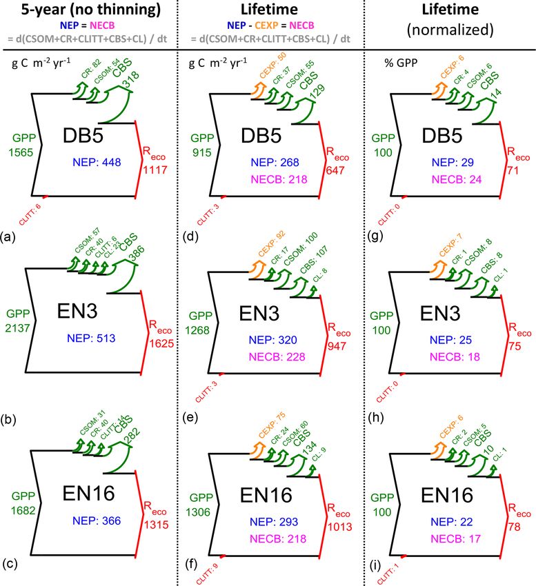
1622                                  C. R. Flechard et al.: Carbon–nitrogen interactions in European ecosystems – Part 2

23 Institute for Geosciences and Environmental research (IGE), UMR 5001, Université Grenoble Alpes, CNRS, IRD,
Grenoble Institute of Technology, 38000 Grenoble, France
24 NRE, Oberwohlenstrasse 27, 3033 Wohlen bei Bern, Switzerland
25 Department of Matter and Energy Fluxes, Global Change Research Centre, AS CR, v.v.i. Belidla 986/4a,

603 00 Brno, Czech Republic
26 Ikerbasque Foundation and Basque Centre for Climate Change, Sede Building 1, Scientific Campus of the University of the

Basque Country, 48940, Leioa, Biscay, Spain
27 Institute of Soil Science and Soil Conservation, iFZ Research Centre for Biosystems, Land Use and Nutrition,

Justus Liebig University Giessen, Heinrich-Buff-Ring 26–32, 35392 Giessen, Germany
28 Institute for Atmospheric and Earth System Research/Forest Sciences, Faculty of Agriculture and Forestry, P.O. Box 27,

00014 University of Helsinki, Helsinki, Finland
29 Earth and Life Institute (Environmental sciences), Université catholique de Louvain, Louvain-la-Neuve, Belgium
30 Institute of Soil Research, Department of Forest and Soil Sciences, University of Natural Resources and Life Sciences

Vienna, Peter Jordan Str. 82, 1190 Vienna, Austria
31 Karlsruhe Institute of Technology (KIT), Institute of Meteorology and Climate Research, Atmospheric Environmental

Research (IMK-IFU), Kreuzeckbahnstr. 19, 82467 Garmisch-Partenkirchen, Germany

Correspondence: Chris R. Flechard (christophe.flechard@inrae.fr)

Received: 23 August 2019 – Discussion started: 11 September 2019
Revised: 9 January 2020 – Accepted: 10 February 2020 – Published: 26 March 2020

Abstract. The effects of atmospheric nitrogen deposition            panied by increasingly large ecosystem N losses by leaching
(Ndep ) on carbon (C) sequestration in forests have often           and gaseous emissions. The reduced increase in productiv-
been assessed by relating differences in productivity to            ity per unit N deposited at high Ndep levels implies that the
spatial variations of Ndep across a large geographic do-            forecast increased Nr emissions and increased Ndep levels in
main. These correlations generally suffer from covariation          large areas of Asia may not positively impact the continent’s
of other confounding variables related to climate and other         forest CO2 sink. The large level of unexplained variability in
growth-limiting factors, as well as large uncertainties in to-      observed carbon sequestration efficiency (CSE) across sites
tal (dry + wet) reactive nitrogen (Nr ) deposition. We propose      further adds to the uncertainty in the dC/dN response.
a methodology for untangling the effects of Ndep from those
of meteorological variables, soil water retention capacity and
stand age, using a mechanistic forest growth model in com-
bination with eddy covariance CO2 exchange fluxes from a            1   Introduction
Europe-wide network of 22 forest flux towers. Total Nr depo-
                                                                    Atmospheric reactive nitrogen (Nr ) deposition (Ndep ) has of-
sition rates were estimated from local measurements as far as
                                                                    ten been suggested to be a major driver of the large forest
possible. The forest data were compared with data from nat-
                                                                    carbon (C) sink observed in the Northern Hemisphere (Reay
ural or semi-natural, non-woody vegetation sites.
                                                                    et al., 2008; Ciais et al., 2013), but this view has been chal-
   The response of forest net ecosystem productivity to nitro-
                                                                    lenged, both in temperate (Nadelhoffer et al., 1999; Lovett
gen deposition (dNEP / dNdep ) was estimated after account-
                                                                    et al., 2013) and in boreal regions (Gundale et al., 2014). In
ing for the effects on gross primary productivity (GPP) of
                                                                    principle, there is a general consensus that N limitation sig-
the co-correlates by means of a meta-modelling standard-
                                                                    nificantly reduces net primary productivity (NPP) (LeBauer
ization procedure, which resulted in a reduction by a factor
                                                                    and Treseder, 2008; Zaehle and Dalmonech, 2011; Finzi et
of about 2 of the uncorrected, apparent dGPP / dNdep value.
                                                                    al., 2007). However, the measure of carbon sequestration is
This model-enhanced analysis of the C and Ndep flux obser-
                                                                    not the NPP, but the long-term net ecosystem carbon balance
vations at the scale of the European network suggests a mean
                                                                    (NECB; Chapin et al., 2006) or the net biome productivity at
overall dNEP / dNdep response of forest lifetime C seques-
                                                                    a large spatial scale (NBP; Schulze et al., 2010), whereby het-
tration to Ndep of the order of 40–50 g C per g N, which is
                                                                    erotrophic respiration (Rhet ) and all other C losses, including
slightly larger but not significantly different from the range of
                                                                    exported wood products and other disturbances over a for-
estimates published in the most recent reviews. Importantly,
                                                                    est lifetime, reduce the fraction of photosynthesized C (gross
patterns of gross primary and net ecosystem productivity ver-
                                                                    primary production, GPP) that is actually sequestered in the
sus Ndep were non-linear, with no further growth responses
                                                                    ecosystem. Indeed, it is possible to view this ratio of NECB
at high Ndep levels (Ndep > 2.5–3 g N m−2 yr−1 ) but accom-
                                                                    to GPP as the efficiency of the long-term retention in the sys-

Biogeosciences, 17, 1621–1654, 2020                                                      www.biogeosciences.net/17/1621/2020/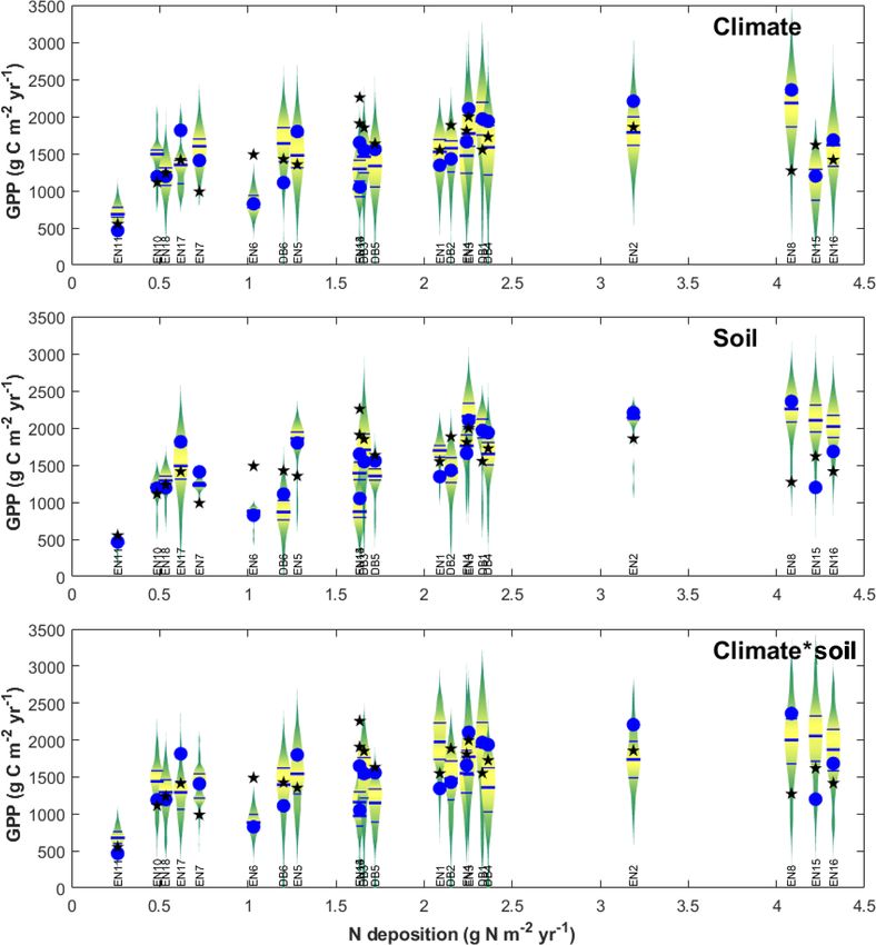
C. R. Flechard et al.: Carbon–nitrogen interactions in European ecosystems – Part 2                                            1623

tem of the assimilated C, in other words a carbon sequestra-        term exposure to excess Nr deposition, would be character-
tion efficiency (CSE = NECB/GPP) (Flechard et al., 2020).           ized by reduced NPP or possibly tree death, even if during
   There is considerable debate as to the magnitude of the          the early or intermediate stages the addition of N could boost
fertilization role that atmospheric Nr deposition may play on       productivity with no visible negative ecosystem impact be-
forest carbon balance, as illustrated by the controversy over       yond NO−   3 leaching. In that initial theory, Aber et al. (1989)
the study by Magnani et al. (2007) and subsequent comments          suggested that plant uptake was the main N sink and led to
by Högberg (2007), De Schrijver et al. (2008), Sutton et            increased photosynthesis and tree growth, while N was re-
al. (2008) and others. Estimates of the dC/dN response (mass        cycled through litter and humus to the available pool; this
C stored in the ecosystem per mass atmospheric N deposited)         fertilization mechanism would saturate quickly, resulting in
vary across these studies over an order of magnitude, from          nitrate mobility. However, observations of large rates of soil
30–70 (de Vries et al., 2008; Sutton et al., 2008; Högberg,         nitrogen retention gradually led to the hypothesis that pools
2012) to 121 (in a model-based analysis by Dezi et al., 2010)       of dissolved organic carbon in soils allowed free-living mi-
to 200–725 g C per g N (Magnani et al., 2007, 2008). Recent         crobial communities to compete with plants for N uptake. A
reviews have suggested mean dC/dN responses generally               revision of that theory by Aber et al. (1998) hypothesized the
well below 100 g C per g N, ranging from 61–98 for above-           important role of mycorrhizal assimilation and root exuda-
ground biomass increment in US forests (Thomas et al.,              tion as a process of N immobilization and suggested that the
2010) to 35–65 for above-ground biomass and soil organic            process of nitrogen saturation involved soil microbial com-
matter (Erisman et al., 2011; Butterbach-Bahl and Gunder-           munities becoming bacterial-dominated rather than fungal or
sen, 2011), 16–33 for the whole ecosystem (Liu and Greaver,         mycorrhizal-dominated in pristine soils.
2009), 5–75 (mid-range 20–40) for the whole ecosystem in               Atmospheric Nr deposition is rarely the dominant source
European forests and heathlands (de Vries et al., 2009), and        of N supply for forests and semi-natural vegetation. Ecosys-
down to 13–14 for above-ground woody biomass in temper-             tem internal turnover (e.g. leaf fall and subsequent decom-
ate and boreal forests (Schulte-Uebbing and de Vries, 2018)         position of leaf litter) and mineralization of SOM provide
and 10–70 for the whole ecosystem for forests globally, in-         annually larger amounts of mineral N than Ndep (although,
creasing from tropical to temperate to boreal forests (de Vries     ultimately, over pedogenic timescales much of the N con-
et al., 2014a; Du and de Vries, 2018).                              tained in SOM is of atmospheric origin). In addition, re-
   A better understanding of processes controlling the dC/dN        sorption mechanisms help conserve within the tree the ex-
response is key to predicting the magnitude of the forest C         ternally acquired N (and other nutrients), whereby N is re-
sink under global change in response to changing patterns           translocated from senescing leaves to other growing parts of
of reactive nitrogen (Nr ) emissions and deposition (Fowler et      the tree, prior to leaf shedding, with resorption efficiencies of
al., 2015). The questions of the allocation and fate of both the    potentially up to 70 % and larger at N-poor sites than at N-
assimilated carbon (Franklin et al., 2012) and deposited ni-        saturated sites (Vergutz et al., 2012; Wang et al., 2013). Bio-
trogen (Nadelhoffer et al., 1999; Templer et al., 2012; Du and      logical N2 fixation can also be significant in forests (Vitousek
de Vries, 2018) appear to be crucial. It has been suggested         et al., 2002). Högberg (2012) showed for 11 European forest
that Nr deposition plays a significant role in promoting the        sites that Nr deposition was a relatively small fraction (13 %–
carbon sink strength only if N is stored in woody tissues with      14 % on average) of the total N supply, which was domi-
high C/N ratios (> 200–500) and long turnover times, as op-         nated by SOM mineralization (up to 15–20 g N m−2 yr−1 ).
posed to soil organic matter (SOM) with C/N ratios that are         He further argued that there may be a correlation between
an order of magnitude smaller (de Vries et al., 2008). Nadel-       soil fertility (of which the natural N supply by mineraliza-
hoffer et al. (1999) argued on the basis of a review of 15 N        tion is an indicator) and Nr deposition, since historically hu-
tracer experiments that soil, rather than tree biomass, was         man populations have tended to develop settlements in areas
the primary sink for the added nitrogen in temperate forests.       of favourable edaphic conditions, in which over time agricul-
However, based on a recent synthesis of 15 N tracer field ex-       ture, industry and population intensified, leading to increased
periments (only including measurements of 15 N recovery af-         emissions and deposition. Thus, an apparent effect of ambi-
ter > 1 year of 15 N addition), Du and de Vries (2018) esti-        ent Ndep on current net ecosystem productivity (NEP) levels
mated that tree biomass was the primary sink for the added          could also be related to the legacy of more than a century of
nitrogen in both boreal and temperate forests (about 70 %),         Nr deposition on a modified internal ecosystem cycle. Im-
with the remaining 30 % retained in soil. At sites with el-         portantly, unlike other ecosystem mechanisms for acquiring
evated N inputs, increasingly large fractions are lost as ni-       N from the environment (resorption from senescing leaves,
trate (NO−  3 ) leaching. Lovett et al. (2013) found in north-      biological N2 fixation, mobilization, and uptake of N from
eastern US forests that added N increased C and N stocks and        soil solution or from SOM), the nitrogen supplied from at-
the C/N ratio in the forest floor but did not increase woody        mospheric deposition comes at little or zero energetic cost
biomass or above-ground NPP.                                        (Shi et al., 2016), especially if absorbed directly at the leaf
   In fact, Aber et al. (1989) even predicted 30 years ago that     level (Nair et al., 2016).
the last stage of nitrogen saturation in forests, following long-

www.biogeosciences.net/17/1621/2020/                                                       Biogeosciences, 17, 1621–1654, 2020
1624                                  C. R. Flechard et al.: Carbon–nitrogen interactions in European ecosystems – Part 2

   Some previous estimates of forest dC/dN response ob-               There are also potentially large uncertainties in the C and
tained by meta-analyses of NEP or NECB across a geo-               N flux measurements or model estimates used to calculate
graphic gradient did not account for the major drivers of          a dC/dN response. In the companion paper (Flechard et al.,
plant growth apart from nitrogen (e.g. Magnani et al., 2007).      2020), we presented – and discussed uncertainties in – plau-
These include climate (precipitation, temperature, photosyn-       sible estimates of C and N budgets of 40 forests and natural
thetically active radiation), soil physical and chemical prop-     or semi-natural ecosystems covering the main climatic zones
erties (e.g. soil drainage, depth, water holding capacity, nu-     of Europe (from Mediterranean to temperate to boreal, from
trients and pH), site history and land use. Using univariate       oceanic to continental), investigated as part of the CarboEu-
statistics such as simple regressions of NECB as a function        rope Integrated Project (CEIP, 2004–2008) and the parallel
of Nr deposition is flawed if Nr deposition is co-correlated       NitroEurope Integrated Project (NEU, 2006–2011). The NEP
with any of these other drivers (Fleischer et al., 2013), as can   budgets were based on multi-annual eddy covariance (EC)
be the case in spatial gradient survey analyses across a wide      datasets following well-established protocols, and in order to
geographic domain. This is because all of the variability in       better constrain the N budgets, specific local measurements
ecosystem C sequestration across the physical space is only        of dry and wet Nr deposition were made. Nitrogen losses by
allowed to be explained by one factor, Nr deposition. For          leaching and gaseous emissions were estimated by a com-
example, Sutton et al. (2008) showed (using forest ecosys-         bination of measurements and modelling. The data showed
tem modelling) that the apparently large dC/dN slope in the        that observation-based GPP and NEP peaked at sites with
dataset of Magnani et al. (2007) was reduced by a factor of        Ndep of the order of 2–2.5 g N m−2 yr−1 but decreased above
2–3 when accounting for climatic differences between sites,        that and that increasingly large Nr losses occurred at larger
i.e. when co-varying limitations in (photosynthetic) energy        Ndep levels, implying that the net dC/dN response was likely
and water were factored out.                                       non-linear, in line with an overview of dC/dN response re-
   Similarly, ignoring the growth stage (forest age) and the       sults from various approaches (De Vries et al., 2014a), pos-
effects of management (thinning) in the analysis introduces        sibly due to the onset of N saturation as predicted by Aber
additional uncertainty in the estimated dC/dN response.            et al. (1989), and associated with enhanced acidification and
Contrasting C-cycling patterns and different N use efficien-       increased sensitivity to drought, frost and diseases (De Vries
cies are expected between young and mature forests. Nutrient       et al., 2014b). The data also showed that, at the scale of the
demand is highest in the early stages of forest development        CEIP–NEU flux tower networks, nitrogen deposition was not
(especially pole stage); a recently planted forest becomes a       independent of climate but peaked in the mid-range for both
net C sink only after a few decades, while at maturity NPP         mean annual temperature and precipitation, which geograph-
and NEP may or may not decrease, depending on a shift              ically corresponds to mid-latitude central and western Eu-
in the balance between autotrophic and heterotrophic respi-        rope, where climate is most conducive to forest productivity
ration (Raut and Rhet , respectively) and GPP (Odum, 1969;         and growth.
Besnard et al., 2018). Thinning can initially increase ecosys-        In the present paper, we further the analysis of the same
tem respiration by increasing litter and SOM stocks and re-        CEIP–NEU observational datasets through forest ecosystem
ducing NPP in the short term, and some biomass can be ex-          modelling, with the objective of isolating the Nr deposition
ported (tree trunks), but the ultimate effect after a year or      impact on forest productivity and C sequestration potential
two is to boost forest growth as thinning indirectly increases     from the parallel effects of climate, soil water retention, and
nutrient availability at the tree level by reducing plant–plant    forest age and management. A mechanistic modelling frame-
competition. Thus, the frequency and intensity of thinning         work, driven by environmental forcings, inputs, growth lim-
will also affect long-term or lifetime NECB. Severe storms,        itations, internal cycling and losses, was required to untan-
fire outbreaks and insect infestations may have a similar ef-      gle the relationships in measurement data, because the ob-
fect.                                                              served dependence of Nr deposition on climate, combined
   Altogether, these complex interactions mean that it is far      with the large diversity but limited number of flux observa-
from a simple task to untangle the Nr deposition effect on         tion sites, restricted the applicability and validity of multi-
ecosystem C sequestration from the impacts of climatic,            variate statistical methods. We describe a methodology to
edaphic and management factors, when analysing data from           derive, through meta-modelling, standardization factors for
diverse monitoring sites situated over a large geographic          observation-based forest productivity metrics, in order to fac-
area (Laubhann et al., 2009; Solberg et al., 2009; Thomas          tor out the part of the variance that was caused by influences
et al., 2010). This is in contrast to fertilization experiments,   other than Nr deposition (climate, soil, stand age). This origi-
where the N effect can be quantified with all other variables      nal meta-modelling approach involves running multiple sim-
being equal between manipulation plots (Nohrstedt, 2001;           ulations of a forest ecosystem model for each site of the flux
Saarsalmi and Mälkönen, 2001), although their results are          tower network, using alternative climate input and soil pa-
only valid for the conditions at the specific location where       rameter data taken from all other sites of the network, in ad-
the experiment has been performed (Schulte-Uebbing and de          dition to each site’s own data. The model results are then
Vries, 2018).                                                      analysed to determine whether conditions at each site are

Biogeosciences, 17, 1621–1654, 2020                                                     www.biogeosciences.net/17/1621/2020/
C. R. Flechard et al.: Carbon–nitrogen interactions in European ecosystems – Part 2                                        1625

likely to be more, or less, favourable to forest growth and       rological data used as ecosystem model inputs (Sect. 2.2),
C sequestration, compared with other sites, from climatic,        were retrieved from the European Fluxes Database Clus-
edaphic and age perspectives, but regardless of atmospheric       ter (2012) and the NEU (2013) database. Dry deposition of
N inputs. This allows the calculation of internal standard-       reactive nitrogen was estimated by measuring at each site
ization factors that are subsequently applied to observational    ambient concentrations of the dominant gas-phase (NH3 ,
flux data within the same collection of sites, aiming to ac-      HNO3 , NO2 ) and aerosol-phase (NH+        −
                                                                                                       4 , NO3 ) Nr concentra-
count for a natural variability that may otherwise bias the       tions (data available from the NitroEurope database; NEU,
analysis of a dC/dN response. Further, we examine patterns        2013), and applying four different inferential models to the
of C and N use efficiencies both at the decadal timescale of      concentration and micro-meteorological data, as described
flux towers and over the lifetime of forests.                     in Flechard et al. (2011). Wet deposition was measured us-
                                                                  ing bulk precipitation samplers (NEU, 2013), with additional
                                                                  data retrieved from national monitoring networks and from
2     Materials and methods                                       the EMEP chemical transport model (CTM; Simpson et al.,
                                                                  2012).
2.1    Carbon and nitrogen datasets from flux tower sites
                                                                  2.2     Modelling of forest carbon and nitrogen fluxes and
Ecosystem-scale carbon fluxes and atmospheric nitrogen de-                pools
position data were estimated within the CEIP and NEU
networks at 31 European forests (6 deciduous broadleaf            2.2.1    General description of the BASFOR ecosystem
forests, DBF; 18 coniferous evergreen needleleaf forests,                  model
ENF, of which 7 were spruce-dominated and 11 were pine-
dominated; 2 mixed needleleaf–broadleaf forests, MF; 5            The BASic FORest (BASFOR) model is a process-based,
Mediterranean evergreen broadleaf forests, EBF) and nine          deterministic forest ecosystem model, which simulates the
short natural or semi-natural (SN) vegetation sites (wetlands,    growth and biogeochemistry (C, N and water cycles) of tem-
peatlands, unimproved and upland grasslands) (Table S1 in         perate deciduous and coniferous stands at a daily time step
the Supplement). In the following we often adopted the            (van Oijen et al., 2005; Cameron et al., 2013, 2018). Model
terminology “observation-based” rather than simply “mea-          code and documentation are available on GitHub (BAS-
sured” to reflect the fact many variables such as GPP or          FOR, 2016). Interactions with the atmospheric and soil en-
below-ground C pools rely on various assumptions or even          vironments are simulated in some detail, including the role
empirical models for their estimation on the basis of mea-        of management (thinning or pruning). BASFOR is a one-
sured data (e.g. flux partitioning procedure to derive GPP        dimensional model, i.e. no horizontal heterogeneity of the
from NEE; allometric relations for tree and root C stocks;        forest is captured, and BASFOR does not simulate some vari-
spatial representativeness of soil core sampling for SOM).        ables which are important in forest production, such as wood
For convenience in this paper, we use the following sign          quality or pests and diseases.
convention for CO2 fluxes: GPP and Reco are both positive,           Nine state variables for the trees describe (i) C pools –
while NEP is positive for a net sink (a C gain from an ecosys-    leaves, branches and stems; roots; and reserves (CL, CB
tem perspective) and negative for a net source.                   and CS or collectively CLBS; CR; CRES; kg C m−2 ); (ii) N
   The general characteristics of the observation sites (coor-    pool in leaves (NL; kg N m−2 ); and (iii) stand density (SD,
dinates, dominant vegetation, forest stand age and height,        trees m−2 ), tree phenology (only for deciduous trees), accu-
temperature and precipitation, Ndep , inter-annual mean C         mulated chill days (d) and accumulated thermal time (Tsum;
fluxes) are provided in Table S1 of the Supplement. The sites,    ◦ C d). Seven state variables for the soil can be divided into

measurement methods and data sources were described in            three categories, according to the three biogeochemical cy-
more detail in the companion paper (Flechard et al., 2020);       cles being simulated: (i) C pools in litter layers of the
for additional information on vegetation, soils, C and N flux     forest floor (CLITT), soil organic matter (SOM) with fast
results and budgets, and their variability and uncertainties      turnover (CSOMF) and SOM with slow turnover (CSOMS)
across the network, the reader is referred to that paper and      (kg C m−2 ); (ii) N pools as for C but also including mineral N
the accompanying supplement. Briefly, the C datasets in-          (NLITT, NSOMF, NSOMS, NMIN; kg N m−2 ); and (iii) the
clude multi-annual (on average, 5-year) mean estimates of         water pool: amount of water to the depth of soil explored by
NEP, GPP and Reco (total ecosystem respiration) based on          the roots (WA; kg H2 O m−2 = mm) (see Table 1).
10–20 Hz EC measurements, post-processing, spectral and              Carbon enters the system via photosynthesis, calculated as
other corrections, flux partitioning, and empirical gap-filling   the product of photosynthetically active radiation (PAR) ab-
(e.g. Lee et al., 2004; Aubinet et al., 2000; Falge et al.,       sorption by the plant canopy and light use efficiency (LUE).
2001; Reichstein et al., 2005; Lasslop et al., 2010). The fully   The leaf and branch pools are subject to senescence, caus-
analysed, validated, gap-filled and partitioned inter-annual      ing carbon flows to litter. Roots are also subject to senes-
mean CO2 fluxes (NEP, GPP, Reco ), as well as the meteo-          cence, causing a flow to fast-decomposing soil organic mat-

www.biogeosciences.net/17/1621/2020/                                                     Biogeosciences, 17, 1621–1654, 2020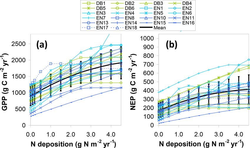
1626                                  C. R. Flechard et al.: Carbon–nitrogen interactions in European ecosystems – Part 2

Table 1. BASFOR model state variables, inputs and outputs, and other acronyms used in the study.

   BASFOR variables                      Description
   Tree state variables
   CL                                    Carbon pool in leaves
   CB                                    Carbon pool in branches
   CS                                    Carbon pool in stems
   CLBS                                  Carbon pool in leaves, branches and stems
   CR                                    Carbon pool in roots
   CRES                                  Carbon pool in reserves
   NL                                    Nitrogen pool in leaves
   SD                                    Forest stand density
   Soil state variables
   CLITT                                 Carbon pool in litter layers
   CSOMF                                 Carbon pool in soil organic matter (fast turnover)
   CSOMS                                 Carbon pool in soil organic matter (slow turnover)
   NLITT                                 Nitrogen pool in litter layers
   NSOMF                                 Nitrogen pool in soil organic matter (fast turnover)
   NSOMS                                 Nitrogen pool in soil organic matter (slow turnover)
   NMIN                                  Soil mineral (inorganic) nitrogen pool
   WA                                    Water pool in the root zone
   Soil parameters
   8SAT                                  Saturation soil water content
   8FC                                   Field capacity
   8WP                                   Wilting point
   ROOTD                                 Root depth
   Model inputs (daily time step)
   Rg                                    Daily global radiation
   Ta                                    Daily average air temperature
   P                                     Daily accumulated rain
   WS                                    Daily average wind velocity
   RH                                    Water vapour pressure
   CO2                                   Annual mean CO2 mixing ratio
   Ndep                                  Annual atmospheric nitrogen deposition
   thinFR                                Fraction of trees removed by thinning
   Model outputs
   H                                     Tree height
   DBH                                   Diameter at breast height
   LAI                                   Leaf area index
   LeafN                                 Leaf N content
   GPP                                   Gross primary productivity
   Reco                                  Ecosystem respiration
   Rhet                                  Soil heterotrophic respiration
   NPP                                   Net primary productivity
   NEE                                   Net ecosystem exchange
   ET                                    Evapotranspiration
   Nminer                                Nitrogen supply from SOM mineralization
   Nupt                                  Root N uptake by trees
   Nleach                                Inorganic N leaching
   NO                                    Nitric oxide
   N2 O                                  Nitrous oxide
   Nemission                             Gaseous soil NO + N2 O emissions

Biogeosciences, 17, 1621–1654, 2020                                                             www.biogeosciences.net/17/1621/2020/
C. R. Flechard et al.: Carbon–nitrogen interactions in European ecosystems – Part 2                                                 1627

Table 1. Continued.

  BASFOR variables                     Description
  Other variables
  GPPobs , NEPobs                      Observation-based (eddy covariance) GPP or NEP
  GPPbase                              Baseline model run for GPP
  GPP∗ , NEP*                          Model-standardized observation-based GPP or NEP
  fCLIM , fSOIL , fAGE                 Model-derived standardization factors to account for climate, soil, age
  NECB                                 Modelled net ecosystem carbon balance, calculated as d(CLBS + CR + CSOM + CLITT)/dt
  Raut                                 Autotrophic respiration
  Rsoil                                Soil (heterotrophic and rhizospheric) respiration
  SCE                                  Soil CO2 efflux measured by chamber methods
  CSEobs                               Observation-based carbon sequestration efficiency (NEPobs /GPPobs )
  CSE5-year, lifetime                  Modelled carbon sequestration efficiency; equal to NEP/GPP (5-year) or NECB/GPP (lifetime)
  NUPE                                 Modelled nitrogen uptake efficiency, calculated as Nupt /Nsupply
  Nsupply                              Total mineral N supply, calculated as (modelled) Nminer + (observation-based)Ndep
  Nloss                                Modelled percentage ecosystem N losses, calculated as (Nleach + Nemission )/Nsupply
  dC/dN, dGPP/dNdep , dNEP/dNdep       Response (slope) of ecosystem C productivity versus atmospheric Nr deposition
  SWHC                                 Soil water holding capacity, = (8FC − 8WP ) × ROOTD
  MAT, MAP                             Mean annual temperature or precipitation
  CEXP                                 Carbon exported by thinning or harvest in forests

ter. Litter carbon decomposes to fast-decomposing soil or-           not be met by supply from the soil, some of the foliar nitro-
ganic matter plus respiration. Fast-decomposing soil organic         gen is recycled until leaves approach a minimum N/C ratio
matter decomposes to slow-decomposing soil organic matter            when leaf senescence will be accelerated. The calculation of
plus respiration. Finally, the slow organic carbon pool de-          foliar senescence accounts for a vertical profile of nitrogen
composes very slowly to CO2 . Nitrogen enters the system             content, such that the lowest leaves have the lowest N/C ra-
in mineral form through atmospheric deposition. Nitrogen             tio and senesce first. Nitrogen deficiency, as measured by fo-
leaves the system through leaching and through emission of           liar nitrogen content, not only increases leaf senescence, but
N2 O and NO from the soil to the atmosphere. N2 losses from          also decreases GPP and shifts allocation from leaves to roots.
denitrification and biological N2 fixation are not simulated.        Given that foliar N content is variable in BASFOR, the litter
Dissolved inorganic nitrogen (DIN) is taken up by the trees          that is produced from leaf fall also has a variable N/C ra-
from the soil, and nitrogen returns to the soil with senescence      tio. When the litter decomposes and is transformed, the N/C
of leaves, branches and roots, and also when trees are pruned        ratio of the new soil organic matter will therefore vary too
or thinned. Part of the N from senescing leaves is reused for        in response to the ratio in the litter. Except for woody plant
growth. The availability of mineral nitrogen is a Michaelis–         parts, the C and N couplings in BASFOR vegetation and soil
Menten function of the mineral nitrogen pool and is propor-          are based on the same generic ecophysiological assumptions
tional to root biomass. The model does not include a dis-            as those explained in detail for the grassland model BAS-
solved organic nitrogen (DON) pool and therefore does not            GRA (Höglind et al., 2020).
account for the possible uptake of bioavailable DON forms               The major inputs to the model are daily time series of
(e.g. amino acids, peptides) by trees. Transformations be-           weather variables (global radiation, air temperature, precip-
tween the four soil nitrogen pools are similar to those of the       itation, wind speed and relative humidity). The last two of
carbon pools, with mineral nitrogen as the loss term. Water is       these are used in the calculation of potential rates of evapora-
added to the soil by precipitation and lost through transpira-       tion and transpiration. Soil properties, such as parameters of
tion, evaporation and drainage. Evaporation and transpiration        water retention (field capacity, wilting point, soil depth), are
are calculated using the Penman equation, as functions of the        provided as constants. Further, the model requires time se-
radiation intercepted by the soil and vegetation layer, and at-      ries indicating at which days the stand was thinned or pruned.
mospheric temperature, humidity and wind speed. Drainage             The model outputs include, amongst others, the state variable
of ground water results from water infiltration exceeding            for trees and soil as well as evapotranspiration (ET), ground-
field capacity of the soil.                                          water recharge, canopy height (H ), leaf area index (LAI),
   In BASFOR, the C and N cycles are coupled in both trees           diameter at breast height (DBH), GPP, Reco and Rsoil , NEP,
and soil. The model assumes that new growth of any or-               N mineralization, N leaching, and NO and N2 O emissions
gan proceeds with a prescribed N/C ratio, which is species-          (Table 1).
specific but generally higher for leaves and roots than for
stems and branches. If the nitrogen demand for growth can-

www.biogeosciences.net/17/1621/2020/                                                         Biogeosciences, 17, 1621–1654, 2020
1628 C. R. Flechard et al.: Carbon–nitrogen interactions in European ecosystems – Part 2
2.2.2 Model implementation and calibration the available density and thinning data for each site, preserv-
ing all actual data in the time series while filling in the gaps
BASFOR simulations of forest growth and C, N and H2 O by plausible interpolation. The density time courses thus ob-
fluxes were made for all CEIP–NEU forest sites from plant- tained, underlying all subsequent model runs, are shown in
ing (spanning the interval 1860–2002) until the end of the Fig. S2.
NEU project (2011). At a few sites, natural regeneration oc- The model was calibrated through a multiple site Bayesian
curred, but for modelling purposes a planting date was as- calibration (BC) procedure, applied to three groups of plant
signed based on the age of the trees. Meteorological data functional types (PFTs), based on C/N/H2 O flux and pool
measured at each site over several years since the establish- data from the CEIP–NEU databases (see Cameron et al.,
ment of the flux towers (typically 5–10 years) were replicated 2018). A total of 22 sites were calibrated, including decid-
backwards in time in order to generate a time series of model uous broadleaf forests (DB1–6) and evergreen needleleaf
inputs for the whole period since planting. Assumptions were forest ENF-spruce (EN1–7) and ENF-pine (EN8–18). The
made that inter-annual meteorological variability was suffi- model parameters were calibrated generically within each
ciently covered in the span of available measurements and PFT group; i.e. they were not optimized or adjusted indi-
that the impact of climate change since planting was small vidually for each observation site. In the companion paper
and could be neglected. (Flechard et al., 2020), baseline BASFOR runs were pro-
The atmospheric CO2 mixing ratio was provided as an ex- duced for all 31 forest sites of the network, including also
ponential function of calendar year, fitted to Mauna Loa data those stands for which the model was not calibrated, such as
since the beginning of records in 1958 (NOAA, 2014) and Mediterranean evergreen broadleaf (EB1 through EB5) and
extrapolated backwards to around 1860–1900 for the oldest mixed deciduous–coniferous (MF1, MF2), to test the pre-
forests included in this study. The global CO2 mixing ra- dictive capacity of the model beyond its calibration range
tio driving the model thus increased from around 290 ppm (see Fig. 6 in Flechard et al., 2020). However, for the anal-
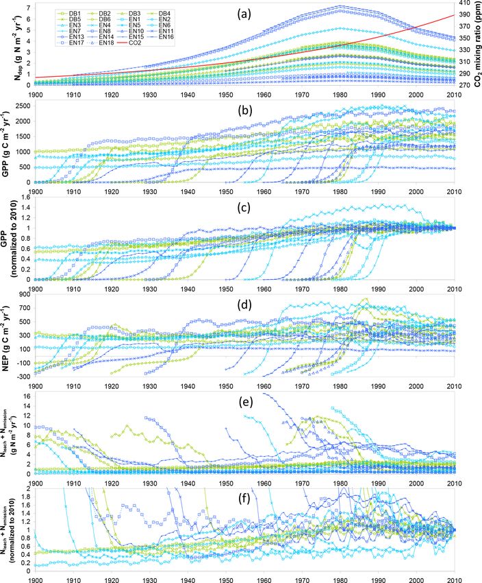
in 1900 to 315 ppm in 1958 to 390 ppm in 2010 (Fig. 1). yses and scenarios presented hereafter, these seven uncali-
Similarly, atmospheric Nr deposition was a key input to the brated sites were removed from the dataset, as were two addi-
model and was forced to vary over the lifetimes of the planted tional sites: EN9 and EN12 – EN9 because this agrosilvopas-
forests; Ndep was assumed to rise from pan-European levels toral ecosystem called “dehesa” has a very low tree density
well below 0.5 g N m−2 yr−1 at the turn of the 20th century, (70 trees ha−1 ; Tables S1–S2 in the Supplement to Flechard
sharply increasing after World War II to reach an all-time et al., 2020) and is otherwise essentially dry grassland for
peak around 1980, and decreasing subsequently from peak much of the surface area, which BASFOR cannot simulate;
values by about one-third until 2005–2010, at which point EN12 because this was a very young plantation at the time of
the NEU Ndep estimates were obtained. We assumed that the measurements, also with a very large fraction of mea-
all sites of the European network followed the same relative sured NEP from non-woody biomass. All the conclusions
time course of Ndep over the course of the 20th century, taken from BASFOR meta-modelling are drawn from the remain-
from van Oijen et al. (2008) but scaled for each site using the ing 22 deciduous, pine and spruce stands (sites highlighted
NEU Ndep estimates (Fig. S1 in the Supplement). in Table S1).
Forest management was included as an input to the model
in the form of a prescribed time course of stand density and 2.2.3 Modelling time frames
thinning from planting to the present date. Tree density was
known at all sites around the time of the CEIP–NEU projects In the companion paper (Flechard et al., 2020), C and N bud-
(Table S2 in Flechard et al., 2020), but information on thin- gets were estimated primarily on the basis of ecosystem mea-
ning history since planting (dates and fractions removed) was surements and for the time horizon of the CEIP and NEU
much sparser. A record of the last thinning event was avail- projects (2004–2010). In this paper, BASFOR simulations of
able at only one-third of all sites, and knowledge of the ini- the C and N budgets for the 22 forest sites were considered
tial (planting) density and a reasonably complete record of both (i) over the most recent 5-year period (around the time
all thinning events were available at only a few sites. For the of CEIP–NEU), which did not include any thinning event
purposes of BASFOR modelling, we attempted to recreate and started at least 3 years after the last thinning event (re-
a plausible density and thinning history over the lifetime of ferred to hereafter as “5-year”); and (ii) over the whole time
the stands. The guiding principle was that after the age of span since forest establishment, referred to here as “lifetime”,
20 years one could expect a decadal thinning of the order of which ranged from 30 to 190 years across the network and
20 %, following Cameron et al. (2013), while the initial re- reflected the age of the stand at the time of the CEIP–NEU
duction was 40 % during the first 20 years. In the absence of projects. Note that the term “lifetime” in this context was not
an actual record of planting density (observed range: 1400– used to represent the expected age of senescence or harvest.
15 000 trees ha−1 ), a default initial value of 4500 trees ha−1 On the one hand, the short-term (5-year) simulations were
was assumed (for around two-thirds of the sites). The gen- made to evaluate cases where no disturbance by management
eral principles of this default scheme were then applied to fit impacted fluxes and pools over a recent period, regardless
Biogeosciences, 17, 1621–1654, 2020 www.biogeosciences.net/17/1621/2020/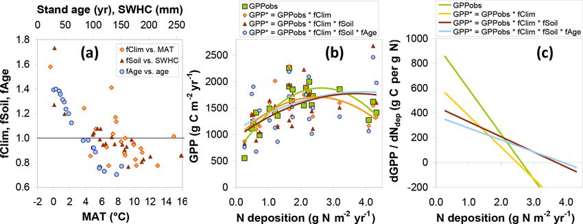
C. R. Flechard et al.: Carbon–nitrogen interactions in European ecosystems – Part 2                                          1629

the age of the stands at the time of the C and N flux mea-        but also the long-term impact of human management through
surements (ca. 2000–2010). On the other hand, the lifetime        thinning frequency and severity.
simulations represent the time-integrated flux and pool his-         For the N budget we define, by analogy to CSE, the N up-
tory since planting, which reflects the long-term C seques-       take efficiency (NUPE) as the ratio of N immobilized in the
tration (NECB) potential, controlled by the cumulative im-        forest system to the available mineral N, i.e. the ratio of tree
pact of management (thinning), increasing atmospheric CO2         N uptake (Nupt ) to the total Nsupply from internal SOM miner-
mixing ratio, and changing Nr deposition over the last few        alization and N-cycling processes (Nminer ) and from external
decades. Thinning modifies the canopy structure and there-        sources such as atmospheric N deposition (Ndep ):
fore light, water and nutrient availability for the trees, and
reduces the LAI momentarily, and in theory the leftover addi-     NUPE = Nupt /Nsupply ,                                       (6)
tional organic residues (branches and leaves) could increase
heterotrophic respiration and affect the NEP. However, the        with
impact of the disturbance on NEP and Reco is expected to
                                                                  Nsupply = Nminer + Ndep ,                                    (7)
be small and short-lived (Granier et al., 2008), and a 3-year
wait after the last thinning event appears to be reasonable for   Nsupply ≈ Nupt + Nleach + Nemission .                        (8)
the modelling. The 5-year data should in theory reflect the
C/N flux observations, although there were a few recorded         The fraction of Nsupply not taken up in biomass and lost to the
thinning events during the CEIP–NEU measurement period,           environment (Nloss ) comprises dissolved inorganic N leach-
and the thinning sequences used as inputs to the model were       ing (Nleach ) and gaseous NO and N2 O emissions (Nemission ):
reconstructed and thus not necessarily accurate (Fig. S2).
                                                                  Nloss = (Nleach + Nemission ) /Nsupply .                     (9)
2.2.4   Modelled carbon sequestration efficiency (CSE)
                                                                  Note that (i) NUPE is a different concept from the nitrogen
        and nitrogen uptake efficiency (NUPE)
                                                                  use efficiency (NUE), often defined as the amount of biomass
For both C and N, we define modelled indicators of ecosys-        produced per unit of N taken up from the soil, or the ratio
tem retention efficiency relative to a potential input level,     NPP/Nupt (e.g. Finzi et al., 2007), and (ii) biological N2 fix-
which corresponds to the total C or N supply, calculated over     ation, as well as N loss by total denitrification, are not ac-
both 5-year (no thinning) and lifetime horizons to contrast       counted for in the current BASFOR version; also, leaching
short-term and long-term patterns. For C sequestration, the       of dissolved organic N and C (DON, DOC) and dissolved
relevant terms are the temporal changes in carbon stocks in       inorganic C (DIC) is not included either, all of which poten-
leaves, branches and stems (CLBS); roots (CR); soil organic       tially impact budget calculations.
matter (CSOM); litter layers (CLITT); and the C export of
                                                                  2.2.5   Meta-modelling as a tool to standardize
woody biomass (CEXP), relative to the available incoming C
                                                                          EC-based productivity data
from gross photosynthesis (GPP). We thus define the carbon
sequestration efficiency (CSE) as the ratio of either modelled    One purpose of BASFOR modelling in this study was to
5-year NEP or modelled lifetime NECB to modelled GPP in           gain knowledge on patterns of C and N fluxes, pools and
a given environment, constrained by climate, nitrogen avail-      internal cycling that were not, or could not be, evaluated
ability and other factors included in the BASFOR model:           solely on the basis of the available measurements (for ex-
CSE5-year (no thinning) = NEP5-year /GPP5-year ,           (1)    ample, SOM mineralization and soil N transfer; retranslo-
                                                                  cation processes at the canopy level; patterns over the life-
CSElifetime = NECBlifetime /GPPlifetime ,                  (2)    time of a stand). The model results were used to complement
with                                                              the flux tower observations to better constrain elemental bud-
                                                                  gets and assess the potential and limitations of C sequestra-
        d (CLBS + CR + CSOM + CLITT)                              tion at the European forest sites considered here. Addition-
NECB =                                 ,                   (3)
                         dt                                       ally, we used meta-modelling as an alternative to multivari-
NECB5-year (no thinning) = NEP5-year ,                     (4)    ate statistics (e.g. stepwise multiple regression, mixed non-
NECBlifetime = NEPlifetime − CEXPthinning .                (5)    linear models, residual analysis) to isolate the importance of
                                                                  Nr deposition from other drivers of productivity. This follows
The modelled CSE5-year can be contrasted with observation-        from the observations by Flechard et al. (2020) that (i) Nr de-
based CSEobs (= NEPobs /GPPobs ) derived from flux tower          position and climate were not independent in the dataset and
data over a similar, relatively short time period compared        that (ii) due to the large diversity of sites the limited size of
with a forest rotation (see Flechard et al., 2020). By exten-     the dataset and incomplete information on other important
sion, the CSElifetime indicator quantifies the efficiency of C    drivers (e.g. stand age, soil type, management), regression
sequestration processes by a managed forest system, reflect-      analyses were unable to untangle these climatic and other
ing not only biological and ecophysiological mechanisms,          inter-relationships from the influence of Nr deposition.

www.biogeosciences.net/17/1621/2020/                                                      Biogeosciences, 17, 1621–1654, 2020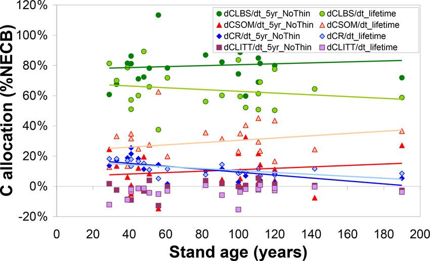
1630                                  C. R. Flechard et al.: Carbon–nitrogen interactions in European ecosystems – Part 2

   BASFOR (or any other mechanistic model) is useful in this        increase and eventual saturation of GPP as Ndep increases be-
context, not so much to predict absolute fluxes and stocks          yond a critical threshold, did not show any marked difference
but to investigate the relative importance of drivers, which        between the three forest PFTs (deciduous, pine, spruce), pos-
is done by assessing changes in simulated quantities when           sibly because the datasets were not large enough and fairly
model inputs are modified. Meta-modelling involves building         heterogeneous. Thus, although PFT may be expected to in-
and using surrogate models that can approximate results from        fluence C–N interactions, we did not seek to standardize GPP
more complicated simulation models; in this case we derived         with an additional fPFT factor.
simplified relationships linking forest productivity to the im-        To determine the fCLIM and fSOIL factors, the model was
pact of major drivers, which were then used to harmonize            run multiple times with all climate and soil scenarios for the
observations from different sites. For example, running BAS-        n (= 22) sites, a scenario being defined as using model in-
FOR for a given site using meteorological input data from           put data or parameters from another site. Specifically, for
another site, or indeed from all other sites of the network,        fCLIM , the model weather inputs at each site were substi-
provides insight into the impact of climate on GPP or NEP,          tuted in turn by the climate data (daily air temperature, global
all other factors (soil, vegetation structure and age, Nr de-       radiation, rainfall, wind speed and relative humidity) from
position) being equal. Within the boundaries of the network         all other sites; and for fSOIL , the field capacity and wilting
of 22 selected sites, this sensitivity analysis provides relative   point parameters (8FC , 8WP ) and soil depth that determine
information as to which of the 22 meteorological datasets is        the soil water holding capacity at each site (SWHC = (8FC −
most, or least, favourable to growth for this particular site.      8WP ) × soil depth) were substituted in turn by parameters
This can be repeated for all sites (22 × 22 climate scenario        from all other sites. Values of fCLIM and fSOIL were calcu-
simulations). It can also be done for soil physical properties      lated for each site in several steps, starting with the calcula-
that affect the soil water holding capacity (texture, porosity,     tion of the ratios of modelled GPP from the scenarios to the
rooting depth), in which case the result is a relative ranking      baseline value GPPbase such that
within the network of the different soils for their capacity to
sustain an adequate water supply for tree growth. The proce-        X(i, j ) = GPP(i, j )/GPPbase (i),                             (11)
dure for the normalization of data between sites is described
                                                                    where i(1. . .n) denotes the site being modelled and j (1. . .n)
hereafter.
                                                                    denotes the climate dataset (jCLIM ) or soil parameter set
   Additional nitrogen affects C uptake primarily through
                                                                    (jSOIL ) used in the scenario being simulated (see Table S2
releasing N limitations at the leaf level for photosynthesis
                                                                    for the calculation matrices). The value of the X(i, j ) ratio
(Wortman et al., 2012; Fleischer et al., 2013), which scales
                                                                    indicates whether the j th scenario is more (> 1) or less (< 1)
up to GPP at the ecosystem level. Other major factors affect-
                                                                    favourable to GPP for the ith forest site.
ing carbon uptake are related to climate (photosynthetically
                                                                       For each site, the aim of the fCLIM factor (and similar rea-
active radiation, temperature, precipitation), soil (for exam-
                                                                    soning for fSOIL ) (Eq. 10) is to quantify the extent to which
ple water holding capacity) or growth stage (tree age). In the
                                                                    GPP differs from a standard GPP∗ value that would occur
following section, we postulate that observation-based gross
                                                                    if all sites were placed under the same climatic conditions.
primary productivity (GPPobs ), which represents an actua-
                                                                    Rather than choose the climate of one particular site to nor-
tion of all limitations in the real world, can be transformed
                                                                    malize to, which could bias the analysis, we normalize GPP
through meta-modelling into a standardized potential value
                                                                    to the equivalent of a mean climate, by averaging BASFOR
(GPP∗ ) for a given set of environmental conditions (climate,
                                                                    results over all (22) climate scenarios (Eqs. 14–15). How-
soil, age) common to all sites, thereby enabling comparisons
                                                                    ever, since each of the scenarios has a different mean impact
between sites. We define GPP∗ as GPPobs being modulated
                                                                    across all sites (X(j ), Eq. 12), we first normalize X(i, j ) to
by one or several dimensionless factors (fX ):
                                                                    the X(j ) value within each j th scenario (Eq. 13):
GPP∗ = GPPobs × fCLIM × fSOIL × fAGE ,                      (10)                  n
                                                                                  X
                                                                    X(j ) = 1/n         X(i, j ),                                  (12)
where the standardization factors fCLIM , fSOIL and fAGE                          i=1
are derived from BASFOR model simulations correspond-               Xnorm (i, j ) = X(i, j )/X(j ).                                (13)
ing to the CEIP–NEU time interval around 2005–2010, as
described below. The factors involved in Eq. (10) address           The normalization of X(i, j ) to Xnorm (i, j ) ensures that the
commonly considered drivers but not nitrogen, which is later        relative impacts of each scenario on all n sites can be com-
assessed on the basis of GPP∗ rather than GPPobs . Other po-        pared between scenarios. The final step is the averaging for
tentially important limitations such as non-N nutrients, soil       each site of Xnorm (i, j ) values from all scenarios (either
fertility, air pollution (O3 ), poor ecosystem health and soil      jCLIM or jSOIL ) into the overall fCLIM or fSOIL values:
acidification are not treated in BASFOR and cannot be quan-                                           n
                                                                                                      X
tified here. Further, the broad patterns of the GPP vs. Ndep re-    fCLIM (i) = Xnorm (i) = 1/n                Xnorm (i, jCLIM )   (14)
lationships reported in Flechard et al. (2020), i.e. a non-linear                                   jCLIM =1

Biogeosciences, 17, 1621–1654, 2020                                                         www.biogeosciences.net/17/1621/2020/
C. R. Flechard et al.: Carbon–nitrogen interactions in European ecosystems – Part 2 1631
or values of the 1980s, added to the internal N supply, were well
n
in excess of growth requirements in the model.
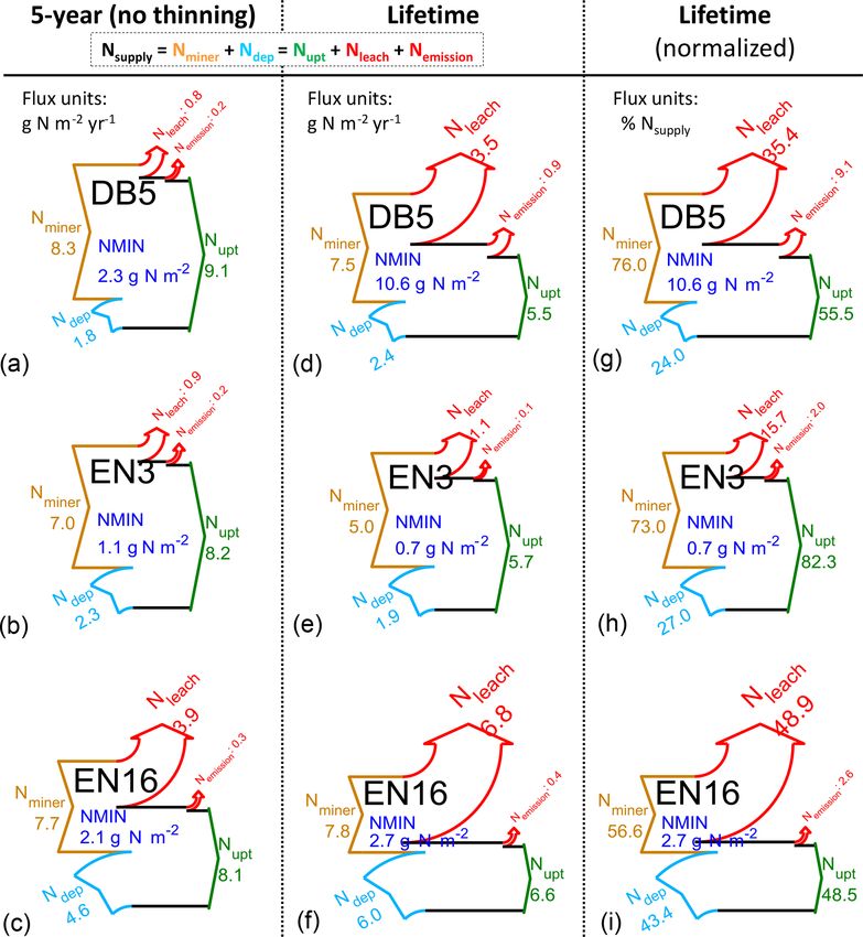
These temporal interactions of differently aged stands with
X
fSOIL (i) = Xnorm (i) = 1/n Xnorm (i, jSOIL ). (15)
jSOIL =1 changing Ndep and CO2 over their lifetimes therefore impact
C- and N-budget simulations made over different time hori-
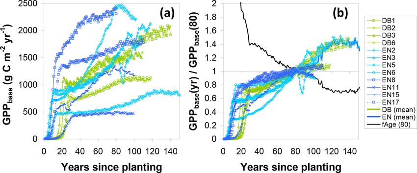
The factors fAGE were determined by first normalizing zons. Modelled C and N budgets are represented schemat-
modelled GPP (base run) to the value predicted at age 80 ically in Figs. 2 and 3, respectively, as Sankey diagrams
for every year of the simulated GPP time series at those m (MATLAB drawSankey.m function; Spelling, 2009) for three
(= 12) mature sites where stand age exceeded 80. The age example forest sites (DB5, EN3, EN16) and in Figs. S3–S8
of 80 was chosen since this was the mean stand age of the of the Supplement for all sites of the study. Each diagram
whole network. The following ratios were thus calculated: represents the input, output and internal flows in the ecosys-
tem, with arrow width within each diagram being propor-
Y (k, yr) = GPPbase (k, yr)/GPPbase (k, 80), (16) tional to flow. For carbon (Figs. 2 and S3–S5), the largest
(horizontal) arrows indicate exchange fluxes with the atmo-
where k(1. . .m) denotes the mature forest site being mod- sphere (GPP, Reco ), while the smaller (vertical) arrows in-
elled. A mean temporal curve for fAGE (normalized to dicate gains (green) or losses (red) in internal ecosystem C
80 years) was calculated to be used subsequently for all sites pools (CSOM, CBS, CR, CL, CLITT), as well as any ex-
using the following: ported wood products (CEXP, orange). NEP is the balance
!−1 of the two horizontal arrows, as well as the balance of all
m
X vertical arrows.
fAGE (yr) = 1/m Y (k, yr) . (17) In the 5-year simulations with no thinning occurring
k=1
(Figs. 2a–c; S3), NEP is equal to NECB, which is the sum
of ecosystem C pool changes over time (equal to C seques-
3 Results tration if positive). By contrast, in the lifetime (since plant-
ing) simulations (Figs. 2d–f; S4), the long-term impact of
3.1 Short-term (5-year) versus lifetime C and N thinning is shown by the additional orange lateral arrow for
budgets from ecosystem modelling C exported as woody biomass (CEXP). In this case, C se-
questration or NECB no longer equals NEP, with the dif-
The time course of modelled (baseline) GPP, NEP, and total ference being CEXP, i.e. the C contained in exported stems
leaching and gaseous N losses is shown in Fig. 1 for all forest from thinned trees. By contrast, in the model, upon thinning
sites over the 20th century and until 2010, forced by climate, the C from leaves, branches and roots joins the litter lay-
increasing atmospheric CO2 and by the assumed time course ers or soil pools and is ultimately respired or sequestered.
of Nr deposition over this period (Fig. 1a). For each stand, To compare between sites with different productivity levels,
regardless of its age and establishment date, an initial phase the lifetime data are also normalized as a percentage of GPP
of around 20–25 years occurs, during which GPP increases (Figs. 2g–i; S5). The clear differences between 5-year and
sharply from zero to a potential value attained upon canopy lifetime C-budget simulations were (i) systematically larger
closure (Fig. 1b), while NEP switches from a net C source to GPP in the recent 5-year horizon (combined effects of age as
a net C sink after about 10 years (Fig. 1d). Initially Nr losses well as CO2 and Ndep changes over time); (ii) C storage in
are very large (typically of the order of 10 g N m−2 yr−1 ) branches and stems (CBS) dominated in both cases, but CBS
and then decrease rapidly to pseudo-steady-state levels when fractions were larger in the 5-year horizon; and (iii) larger
GPP and tree N uptake reach their potential. relative storage in soil organic matter (CSOM) when calcu-
After this initial phase, modelled GPP increases steadily in lated over lifetime.
response to increasing Ndep and atmospheric CO2 , but only For nitrogen, in contrast to carbon, the focus of the budget
for the older stands established before around 1960, i.e. those diagrams is not on changes over time of the total ecosys-
stands that reach canopy closure well before the 1980s, when tem (tree + soil, organic + mineral) N pools. Rather, we ex-
Nr deposition is assumed to start declining. Thereafter, mod- amine in Figs. 3 and S6–S8 the extent to which Nr depo-
elled GPP ceases to increase, except for the recently estab- sition contributes to the mineral N pool (NMIN), which in
lished stands that have not yet reached canopy closure. The the model is considered to be the only source of N available
stabilization of GPP for mature trees at the end of the 20th to the trees and therefore acts as a control of C assimilation
century in the model is likely a consequence of the effects and ultimately sequestration. In these diagrams for NMIN,
of decreasing Ndep and increasing CO2 cancelling each other the largest (horizontal) arrows indicate the modelled internal
out to a large extent. In parallel, modelled total N losses start ecosystem N-cycling terms (Nminer from SOM mineraliza-
to decrease after the 1980s, even for sites long past canopy tion, Nupt uptake by trees), and the secondary (vertical) ar-
closure (Fig. 1e–f), but this mostly applies to stands subject rows represent external exchange (inputs and losses) fluxes
to the largest Ndep levels, i.e. where the historical high Ndep as Ndep , Nleach and Nemission (unit: g N m−2 yr−1 ). The vari-
www.biogeosciences.net/17/1621/2020/ Biogeosciences, 17, 1621–1654, 2020You can also read