Progress in Oceanography - Contents lists available at ScienceDirect - University of Glasgow
←
→
Page content transcription
If your browser does not render page correctly, please read the page content below
Progress in Oceanography 198 (2021) 102657
Contents lists available at ScienceDirect
Progress in Oceanography
journal homepage: www.elsevier.com/locate/pocean
The summer distribution, habitat associations and abundance of seabirds in
the sub-polar frontal zone of the Northwest Atlantic
Ewan D. Wakefield a, *, David L. Miller b, Sarah L. Bond c, Fabrice le Bouard d,
Paloma C. Carvalho e, Paulo Catry f, Ben J. Dilley g, David A. Fifield h, Carina Gjerdrum i,
Jacob González-Solís j, Holly Hogan k, Vladimir Laptikhovsky l, Benjamin Merkel m, Julie A.
O. Miller a, Peter I. Miller n, Simon J. Pinder a, Tânia Pipa o, Peter M. Ryan g,
Laura A. Thompson p, Paul M. Thompson q, Jason Matthiopoulos a
a
University of Glasgow, Institute of Biodiversity, Animal Health and Comparative Medicine, Graham Kerr Building, Glasgow G12 8QQ, UK
b
Centre for Research into Ecological and Environmental Modelling and School of Mathematics and Statistics, University of St Andrews, The Observatory, Buchanan
Gardens, St Andrews, Fife KY16 9LZ, UK
c
School of Ocean Sciences, Bangor University, Menai Bridge, Anglesey LL59 5AB, UK
d
RSPB Centre for Conservation Science, Royal Society for the Protection of Birds, The Lodge, Sandy, Beds, SG19 2DL, UK
e
Centre for Earth Observation Science (CEOS), University of Manitoba, Winnipeg-MB, MB R3T 2N2, Canada
f
Marine and Environmental Sciences Centre (MARE), ISPA - Instituto Universitário, Rua Jardim do Tabaco 34, 1149-041 Lisbon, Portugal
g
FitzPatrick Institute of African Ornithology, DST/NRF Centre of Excellence, University of Cape Town, Rondebosch 7701, South Africa
h
Wildlife Research Division, Science and Technology Branch, Environment and Climate Change Canada, Mount Pearl, NL, Canada
i
Canadian Wildlife Service, 45 Alderney Drive, Dartmouth, NS B2Y 2N6, Canada
j
Institut de Recerca de la Biodiversitat (IRBio) and Department de Biologia Evolutiva, Ecologia i Ciències Ambientals (BEECA), Universitat de Barcelona, Barcelona,
Spain
k
Independent researcher, 29 Connemara Place, St. John’s, NL A1A 3E3, Canada
l
Centre for Environment, Fisheries and Aquaculture Science, Pakefield Road, Lowestoft NR33 0HT, UK
m
Akvaplan-niva, Fram Centre, PO Box 6606 Langnes, 9296 Tromsø, Norway
n
Remote Sensing Group, Plymouth Marine Laboratory, Prospect Place, Plymouth PL1 3DH, UK
o
Portuguese Society for the Study of Birds, Lisbon, Portugal
p
School of Geographical and Earth Sciences, University of Glasgow, Glasgow G12 8QQ, UK
q
Lighthouse Field Station, School of Biological Sciences, University of Aberdeen, Cromarty, Ross-shire IV11 8YL, UK
A R T I C L E I N F O A B S T R A C T
Keywords: Biological production in the oceanic zone (i.e. waters beyond the continental shelves) is typically spatially patchy
Distance sampling and strongly seasonal. In response, seabirds have adapted to move rapidly within and between ocean basins,
Habitat model making them important pelagic consumers. Studies in the Pacific, Southern and Indian Oceans have shown that
Mesoscale eddy
seabirds are relatively abundant in major frontal systems, with species composition varying by water mass. In
Marine protected area
Procellariiformes
contrast, surprisingly little was known about seabird distribution in the oceanic North Atlantic until recent
Shearwater tracking showed that relative abundance and diversity peak in the Sub-polar Frontal Zone, west of the Mid-
Atlantic Ridge, now proposed as a Marine Protected Area. However, absolute seabird abundance, distribution,
age and species composition, and their potential environmental drivers in the oceanic temperate NW Atlantic
remain largely unknown. Consequently, we systematically surveyed seabirds and environmental conditions
across this area by ship in June 2017, then modelled the density of common species as functions of environ
mental covariates, validating model predictions against independent tracking data. Medium-sized petrels
(99.8%), especially Great Shearwaters (Ardenna gravis, 63%), accounted for the majority of total avian biomass,
which correlated at the macroscale with net primary production and peaked at the sub-polar front. At the
mesoscale, the density of each species was associated with sea surface temperature, indicating zonation by water
mass. Most species also exhibited scale-dependent associations with eddies and fronts. Approximately 51, 26, 23,
7 and 1 % of the currently estimated Atlantic populations of Cory’s Shearwaters (Calonectris borealis), Great
Shearwaters, Sooty Shearwaters (A. grisea), Northern Fulmars (Fulmarus glacialis) and Leach’s Storm-petrels
* Corresponding author.
E-mail address: Ewan.Wakefield@glasgow.ac.uk (E.D. Wakefield).
https://doi.org/10.1016/j.pocean.2021.102657
Received 30 April 2021; Received in revised form 17 July 2021; Accepted 3 August 2021
Available online 8 August 2021
0079-6611/© 2021 The Authors. Published by Elsevier Ltd. This is an open access article under the CC BY license (http://creativecommons.org/licenses/by/4.0/).
E.D. Wakefield et al. Progress in Oceanography 198 (2021) 102657
(Oceanodroma leucorhoa) occurred in the area during our survey, many of which were undergoing moult (a vital
maintena nce activity). For some species, these estimates are higher than suggested by tracking, probably due to
the presence of immatures and birds from untracked populations. Our results support the conclusion that MPA
status is warranted and provide a baseline against which future changes can be assessed. Moreover, they indicate
potential drivers of seabird abundance and diversity in the oceanic zone of the North Atlantic that should be
investigated further.
1. Introduction seabirds over the deep North Atlantic has renewed. Synthesis of tracking
data from multiple populations has shown that at least 21 species,
The oceanic zone (i.e. waters beyond the continental shelves) is the originating from breeding locations as far apart as the Arctic (Gilg et al.,
largest habitat on Earth. It remains relatively poorly understood but is 2013) and Antarctica (Kopp et al., 2011), aggregate in a relatively small
undergoing increasingly rapid human exploitation (Crespo et al., 2018; (0.5 million km2) part of this area, west of the mid-Atlantic ridge (MAR),
St. John et al., 2016). For example, although seabirds are among its most centred at ~37◦ W, 50◦ N (Davies et al., 2021). This includes breeding
conspicuous inhabitants, their abundance and relationships with adults that routinely commute from northern hemisphere colonies to
oceanographic processes in the open ocean remain poorly known forage in the area during the boreal summer (Edwards et al., 2013; Paiva
(Rodríguez et al., 2019). Reducing this uncertainty is important because et al., 2010a); North Atlantic breeders making stopovers during migra
seabirds are major consumers in pelagic ecosystems (Barrett et al., 2006; tions to and from southern hemisphere non-breeding areas (Egevang
Brooke, 2004b; Hunt and McKinnell, 2006), recycle otherwise limiting et al., 2010; Freeman et al., 2013); and adults from colonies in the
nutrients (Savoca, 2018; Shatova et al., 2017), and are hyper-mobile northern (Fayet et al., 2017; Fort et al., 2012; Frederiksen et al., 2012)
(Dias et al., 2012; Edwards et al., 2013; Hedd et al., 2012; Kopp et al., and southern hemisphere (Hedd et al., 2012; Kopp et al., 2011) that
2011), linking disparate marine and terrestrial ecosystems with impor spend some or all of their respective non-breeding periods in the area.
tant biological and economic consequences (Plazas-Jiménez & Cian Seabird abundance in the area is relatively high year-round (Davies
ciaruso, 2020). Additionally, not only do seabirds consume a similar et al., 2021). In the boreal winter, the avifauna is dominated by alcids,
amount to human fisheries, they are also bycaught in those fisheries, especially the Little Auk (Alle alle), and Black-legged Kittiwakes (Rissa
leading to widespread and unsustainable population declines (Croxall tridactyla) (Fauchald et al., 2021; Fort et al., 2012; Frederiksen et al.,
et al., 2012; Cury et al., 2011; Dias et al., 2019; Grémillet et al., 2018). 2012). In in the boreal summer, diversity is higher and medium-sized
They are also likely to be vulnerable to the large-scale effects of climate petrels, especially Great Shearwaters (Ardenna gravis), predominate
change (Dias et al., 2019; Rodríguez et al., 2019). Given the rapid (Davies et al., 2021). It has also been inferred from biologging data that
changes the marine environment is undergoing, which are likely to many species undergo moult in the area (Hedd et al., 2012; Kopp et al.,
intensify in the next decades, it is urgent to quantify seabird abundance 2011), which is a vital maintenance activity for birds (Ellis & Gabrielsen,
in the open ocean to establish current baseline levels, at least in major 2002).
hotspots. Moreover, in order to conserve seabirds effectively, it is It has been recognised that the area of highest seabird concentration
necessary to understand relationships with environmental drivers and coincides with the sub-polar frontal zone (hereafter, SPFZ) (Boertmann,
underlying processes driving seabird abundance and distribution 2011; Skov et al., 1994; Davies et al., 2021), which in the NW Atlantic is
(Grémillet & Boulinier, 2009). an area of particularly dynamic physical oceanography (see Section 2).
Pioneering investigations of seabird distributions in the oceanic zone The SPFZs of the Pacific and Southern Oceans also sustain high seabird
were carried out in the North Atlantic, demonstrating, for example, a diversity and abundance and seabird-habitat associations in these sys
macroscale correlation between seabird and phytoplankton abundance tems have been studied extensively in situ (Ainley & Boekelheide, 1984;
and the influx and movements of southern hemisphere migrants during Hyrenbach et al., 2007; Pakhomov & McQuaid, 1996; Wahl et al., 1989).
the boreal summer (Jespersen, 1924; Jespersen, 1930; Wynne-Edwards, In contrast, at-sea studies of seabirds in the NW Atlantic SPFZ have been
1935). Since then however, ship-based investigations into seabird- limited in extent and restricted mainly to descriptions of occurrence and
habitat relationships in the oceanic zone have focussed on the Pacific, relative density (Bennison & Jessopp, 2015; Boertmann, 2011; Brown,
Indian and Southern Oceans (Ainley & Boekelheide, 1984; Ballance 1986). Only one previous ship-based study described seabird habitat
et al., 2006; Hyrenbach et al., 2007; Pakhomov & McQuaid, 1996; use, and this covered only a small part of the SPFZ (Skov et al., 1994).
Springer et al., 1999; Wahl et al., 1989). These studies, augmented more Furthermore, despite numerous recent tracking studies showing that
recently by seabird tracking and satellite remote sensing, indicate that seabirds use the deep NW Atlantic, tracking has only been used to
seabird-habitat relationships in the oceanic zone are scale-dependent quantify habitat use by alcids, which predominantly occur in the area in
(Fauchald et al., 2000; Pakhomov & McQuaid, 1996; Ribic et al., the winter, and Cory’s Shearwaters (Calonectris borealis) (Fort et al.,
1997). At the macroscale (throughout, we use terms defined by Haury 2012; Merkel et al., 2021; Paiva et al., 2010a; Paiva et al., 2010b;
et al.’s (1977) when referring to spatial scale), community composition Tranquilla et al., 2015). These studies suggest that seabird distribution
reflects productivity, water masses and proximity to breeding colonies. in NW Atlantic may vary systematically with water mass. However,
Abundance is highest in the major frontal systems, in upwellings asso relationships between most species and fronts, mesoscale turbulence,
ciated with eastern boundary currents, and seasonally, at high latitudes primary production, etc., especially in the summer, when medium sized
(Ainley & Boekelheide, 1984; Ballance et al., 2006; Hyrenbach et al., petrels predominate, remain essentially unknown, hindering our un
2007; Pakhomov & McQuaid, 1996; Pocklington, 1979; Springer et al., derstanding of the drivers of high seabird abundance in the area.
1999; Wahl et al., 1989). At finer scales, fronts, eddies, internal waves, The core region of high seabird abundance and diversity identified
etc., as well as the behaviour of prey, give rise to a nested hierarchy of by Davies et al. (2021) is currently being considered by the OSPAR
prey patches (Bertrand et al., 2014; Bost et al., 2009; Fauchald, 2009; Commission as a potential Marine Protected Area (the North Atlantic
Haney, 1986; Scales et al., 2014; Tew Kai & Marsac, 2010). However, Current and Evlanov Seamount Marine Protected Area – hereafter
mismatches between seabirds, their prey and physical drivers can occur NACES pMPA, Fig. 1). However, until recently, it was largely imprac
at the mesoscale and below due to trophic lags, social effects, compe ticable to track immature seabirds, so the data used to identify this area
tition, etc. (Grémillet et al., 2008; Hunt et al., 1999; Veit & Harrison, pertain only to adults. Approximately half of pelagic seabirds are im
2017). matures (Brooke, 2004a; Carneiro et al., 2020), which can have mark
In recent years, due to the burgeoning of tracking studies, interest in edly different distributions to adults (Campioni et al., 2020; Carneiro
2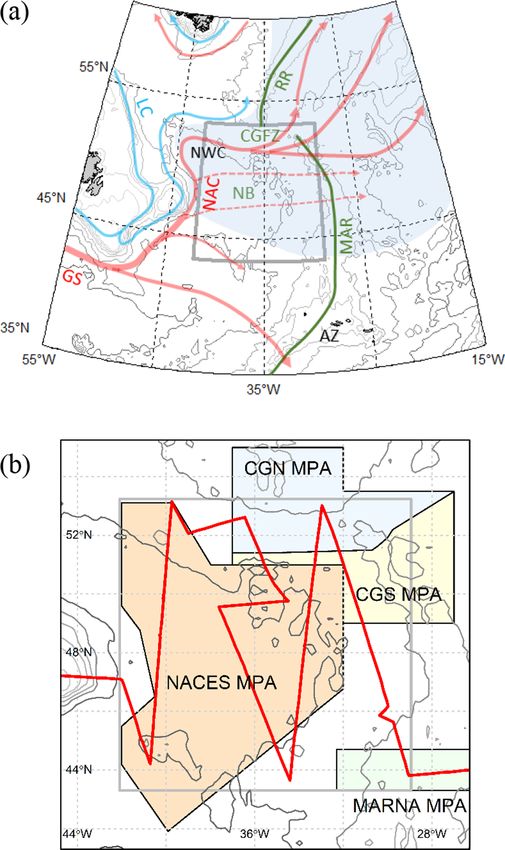
E.D. Wakefield et al. Progress in Oceanography 198 (2021) 102657
et al., 2017).
Here, we report the findings of the first widescale survey of seabirds
in the SPFZ of the NW Atlantic, carried out in June 2017. Our primary
aims were to (1) quantify the habitat associations of the commonest
species in the area (Northern Fulmars, Cory’s Shearwaters, Great
Shearwaters, Sooty Shearwaters (A. grisea) and Leach’s Storm-petrels
(Oceanodroma leucorhoa) - hereafter NOFU, COSH, GRSH, SOSH and
LHSP, respectively), and (2) estimate their distribution and abundance
(individuals and biomass), both in the area as a whole and within the
NACES pMPA. In addition, we report the moult status and age of sea
birds in the area and the occurrence of less abundant species.
2. Physical and biogeographic setting
We defined our study area (Fig. 1; 43◦ 18ʹ to 53◦ 12ʹN, 29◦ 0ʹ to
42◦ 6ʹW; extent 1,174,800 km2) to encompass the seabird diversity and
abundance hotspot identified by Davies et al. (2021). This area occupies
much of the Newfoundland Basin and is bounded to the east by the MAR,
to the north by the Charlie-Gibbs Fracture Zone (CGFZ - a large
discontinuity in the MAR/Reykjanes Ridge) and to the west by the North
American continental rise. Its mean depth is 3814 m (range 907–5031
m) but many shallower seamounts occur, mainly towards the northern,
eastern and southwestern margins. The region’s physical oceanography
was reviewed by Rossby (Rossby, 1996). In brief, surface transport is
dominated by the warm North Atlantic Current (NAC), which branches
from the Gulf Stream SE off the Grand Banks. From there, the NAC
follows the continental rise around the Flemish Cap, before retroflecting
sharply north-westwards then eastwards (thus forming the “Northwest
Corner”), passing through the CGFZ, and continuing NE beyond the
study area. The cold, southward flowing Labrador Current meets the
NAC south of the Flemish Cap, returning north-eastwards with the latter.
In the upper ocean (0–1000 m), the SPFZ is characterised by a stepped
transition from warm/saline subtropical North Atlantic Central Water
(NACW; SST > 15 ◦ C, S > 35.5) in the south to colder/fresher Sub-Arctic
Intermediate Water (SAIW; SST < 10 ◦ C, S < 35.0) in the north (defi
nitions based on Cook et al. (2013), Søiland et al. (2008) and observa
tions made during our study). West of the MAR, the NAC forms at least
three approximately parallel, zonally aligned jets and associated fronts
(Belkin & Levitus, 1996; Bower & von Appen, 2008; Miller et al., 2013b;
Fig. 1. The study area (grey polygon). (a) Major bathymetric features (green) Søiland et al., 2008). The subpolar front has two components - the North
and surface currents (red/warm, blue/cold). Dashed red lines indicate tran
Subpolar Front (NSPF) and South Subpolar Front (SSPF). South of this is
sient, eastward flowing branches of the North Atlantic Current (NAC) and light
the less clearly defined Mid-Atlantic Front (MAF) (Belkin & Levitus,
blue shading the subpolar frontal zone. Abbreviations are AZ, Azores; CGFZ,
Charlie-Gibbs Fracture Zone; GS, Gulf Stream; LC, Labrador Current; MAR, Mid-
1996; Miller et al., 2013b). The NSPF typically crosses the MAR at the
Atlantic Ridge; NB, Newfoundland Basin; NWC, Northwest Corner; and RR, CGFZ but the other fronts are more variably associated with fracture
Reykjanes Ridge. Isobaths indicate 50, 100, 200, 500, 1000, 2000, 3000, 4000 zones in the MAR (Bower & von Appen, 2008). Mesoscale turbulence
and 5000 m depth. Based on Sy (1988), Rossby (1996), Belkin and Levitus within the SPFZ is high (Chelton et al., 2011; Miller et al., 2013b; Til
(1996) and Søiland et al. (2008) and the current study. (b) Detail of study area stone et al., 2014) and upper water masses between the MAF and sub
in the Lambert Azimuthal Equal Area projection used in the remaining figures, polar fronts comprise a matrix of NACW, SAIW, and intermediate water,
showing the cruise track (red) and existing/proposed Marine Protected Areas: which together we refer to as Frontal Water (FW) (Cook et al., 2013;
CGN, Charlie-Gibbs North MPA; CGS, Charlie-Gibbs South MPA; NACES, North Søiland et al., 2008).
Atlantic Current and Evlanov Seamount proposed MPA; MARNA, Mid-Atlantic Biogeographically, the area is characterised by high summer primary
Ridge North of the Azores MPA. (For interpretation of the references to colour
production associated with lateral stirring across the SPF (Longhurst,
in this figure legend, the reader is referred to the web version of this article.)
1998; Tilstone et al., 2014) and a complex mosaic of pelagic habitats
(Beaugrand et al., 2019). The SPFZ acts as both a biogeographical bar
et al., 2020; Powers et al., 2020). Similarly, tracking data are lacking for rier separating communities associated with SAIW (relatively low di
many populations that potentially use the area (e.g. Northern Fulmars versity/high abundance) and NACW (relatively high diversity/low
Fulmarus glacialis from NW Atlantic colonies), including those of most abundance), and an ecotone with higher abundance at all trophic levels
smaller species, such as the storm-petrels (Hydrobatidae/Oceanitidae). and its own distinct faunal assemblage (Beaugrand et al., 2002; Vec
Ship-based surveys, combined with onboard oceanographic sampling, chione et al., 2010a; Vecchione et al., 2015). Two major ecoregions have
satellite remote-sensing and habitat modelling, can be used to both been recognised (Beaugrand et al., 2019; Sutton et al., 2017): To the
quantify seabird-habitat associations and estimate their abundance north, the Sub-Polar Oceanic (Beaugrand et al’s terminology), with
(Buckland et al., 2016; Miller et al., 2013a; Waggitt et al., 2020), vali relatively low zooplankton diversity but high abundance of the copepod
dating estimates inferred indirectly from tracking data (Carroll et al., Calanus finmarchicus and Hyperiid amphipods. To the south, the Oceanic
2019; Louzao et al., 2009). For some species, at sea surveys also allow Warm-Temperate has a more diverse copepod and diatom community
age and moult status to be observed or inferred, providing information and lower seasonal variation in abundance. There are few data on
that is difficult to collect remotely (Brown, 1988; Keijl, 2011; Meier mesotrophic fauna in the area itself but extensive investigations during
3
E.D. Wakefield et al. Progress in Oceanography 198 (2021) 102657
the MAR-ECO project (Priede et al., 2013; Vecchione et al., 2010a), deployed Time-Depth Recorders (TDRs) on a subsample of the tracked
conducted over the MAR immediately to the east suggest that Mycto shearwaters. We tracked NOFU from Eynhallow, Scotland (59◦ 8′ N,
phids dominate above 750 m, with shrimps and cephalopods also rela 3◦ 8′ W); GRSH from Gough, South Atlantic (40◦ 19′ S, 9◦ 56′ W); and SOSH
tively abundant (Cook et al., 2013; Sutton et al., 2013; Vecchione et al., from Kidney Island, Falkland Islands (51◦ 38′ S, 57◦ 45′ W) for ≥ one year
2010b). overlapping with the survey period. For logistical reasons, it was not
possible to deploy loggers on COSH prior to the survey. Rather, we
3. Methods tracked this species from Corvo, Azores (39◦ 41′ N, 31◦ 7′ W) for one year,
commencing immediately after the survey. It was not known that LHSP
To estimate seabird distribution and abundance and investigate are one of the most abundant species in the study area until the survey
habitat associations within the study area, we surveyed birds by ship was carried out, so we did not track this species. Loggers were deployed
using standard methods (Camphuysen et al., 2004; Tasker et al., 1984; and recovered on NOFU as described by Grissot et al. (2020) and on
Webb & Durinck, 1992), while simultaneously measuring sea surface shearwaters as described by Bonnet-Lebrun et al. (2020) (Supplemen
properties in situ and via satellite. We then modelled seabird density as a tary Methods for details).
function of environmental covariates to infer habitat associations and
predict seabird distribution and abundance across the study area. To 3.3. Modelling detection probability
validate these models against independent observations, we also tracked
representative samples of four species (NOFU, COSH, GRSH and SOSH) We used model-based distance sampling (Miller et al., 2013a) to
that were abundant during the at-sea survey.
estimate the distribution and abundance of the most abundant species (i.
e. those with ≥ 60 detections, which is the minimum required to esti
3.1. Ship-based seabird survey mate a robust detection function (Buckland et al., 2001)). We assumed
that the probability of detecting birds on the water declines with dis
We surveyed seabirds from the RRS Discovery (cruise DY080) be tance from the transect line and with sea and weather conditions. We
tween the 13th and 29th of June 2017. A sawtooth survey pattern, used the R package Distance (Miller et al., 2019) to model detectability
comprising five transects running perpendicular to the major fronts
and estimate the probability of detection ̂ p w , considering various stan
within the study area, was planned but this was modified during the
dard functional forms (Marques et al., 2007), as well as the following
cruise in order to sample a transient phytoplankton bloom in the NW of
covariates - wind speed, wave height, visibility (all continuous) and
the study area (Fig. 1). We used the Eastern Canada Seabirds At Sea
precipitation (binary). We recorded distances in one of four bands, so we
(ECSAS) protocol (Gjerdrum et al., 2012). This follows de facto standard
limited the maximum number of parameters in detection functions to
methods for surveying seabirds from ships (Camphuysen et al., 2004;
three. We therefore considered models with up to two covariates using
Tasker et al., 1984; Webb & Durinck, 1992), comprising a simultaneous
half-normal and hazard-rate detection functions, plus models with no
line transect survey for birds on the water, a strip transect survey for
covariates but including adjustment terms to improve fit, selecting
birds in flight (transect width of 300 m) and periodic recording of
among these models based on their AIC. As distances occurred in four
weather conditions that may affect seabird detectability (see Supple
bins, it was not possible to obtain χ 2 goodness-of-fit statistics, so we
mentary Methods). Movement of flying birds relative to the ship can bias
assessed model fit visually by plotting the observed frequency of de
density estimates (Gaston et al., 1987). To minimise this effect, we used
tections vs. distance, overlaid with the fitted detection functions. There
a ‘snapshot’ method to record birds first detected in flight, flagging re
were insufficient detections of SOSH and COSH to fit robust detection
cords of flying birds if they were within a 300 × 300 m box at the
models for these species separately, but SOSH, COSH and GRSH have a
moment of the snapshot (Tasker et al., 1984). We used only records of
similar, predominantly dark, appearance on the water so we pooled
birds in flight at snapshots (hereafter, in-flight), plus all sightings of birds
detections of these species and fitted a generic detection function for all
on the water (hereafter, on-water) to estimate density. Together, we refer
shearwaters.
to these as ‘in-transect’ sightings. We noted if birds were obviously
We assumed that the probability ̂ p f of detecting the larger species
following the ship and excluded these records from the density analysis.
In order to obtain an approximate estimate of the moult status of birds in (NOFU and the shearwaters) in flight was uniform within the surveyors’
the study area, whenever possible we examined birds using binoculars search area (Waggitt et al., 2020). LHSP are, in contrast, much smaller
and recorded whether they were clearly in active primary moult (i.e., and usually fly closer to the water than these species, making them more
one or more primaries missing or not fully grown). We recorded the difficult to detect. Moreover, they forage predominantly by foot pat
colour phase of NOFU on the four point scale described by van Franeker tering or otherwise remaining in partial contact with the sea (Flood &
and Wattel (1982), where birds with the lightest and darkest plumage Fisher, 2011), so it was often ambiguous whether detections should be
are termed LL and DD, respectively, and lighter and darker in classed as in flight or on the surface. However, this behaviour makes it
termediates are termed L and D, respectively. We also recorded the practicable to estimate the distance of LHSP from the transect line using
approximate age (calendar year) of gannets, gulls, terns and skuas when the Heinemann (1981) technique. We therefore fitted a detection
this could be discriminated from plumage. function to pooled in-flight and on-water detections for this species.
3.2. Seabird tracking 3.4. Explanatory environmental covariates
In order to obtain an independent estimate of the distribution of the We modelled the density of seabirds (see Section 3.5) as functions of
most abundant seabird species in the study area during the ship-based three types of candidate explanatory covariates (Table 1): (1) Accessi
survey, we used light-based geolocation loggers to track these species bility from breeding colonies; (2) indices describing environmental
from their breeding colonies. We then compared the distributions pre phenomena or properties that could affect prey distribution; and (3)
dicted by models fitted to the at-sea survey data to these data (see spatial location (see Section 3.7). These covariates were either measured
Section 5.1 for caveats). It was only practicable to track birds from one shipboard during the survey (hereafter, locally-sensed), and therefore
colony per species. We selected these colonies based on prior under relatively high-resolution but available only along the cruise track, or
standing of which populations were likely to use the study area during remotely-sensed at lower resolution across the whole study area.
the survey (Edwards et al., 2013; Hedd et al., 2012; Magalhaes et al., We considered the following indices: Accessibility (α), which for
2008; Paiva et al., 2010a,b; Davies et al., 2021) and logistical con species breeding at the time of the survey (NOFU, COSH and LHSP), we
straints. In addition, to account for availability bias (see Section 3.7), we define as the inverse of the great circle distance to their nearest breeding
4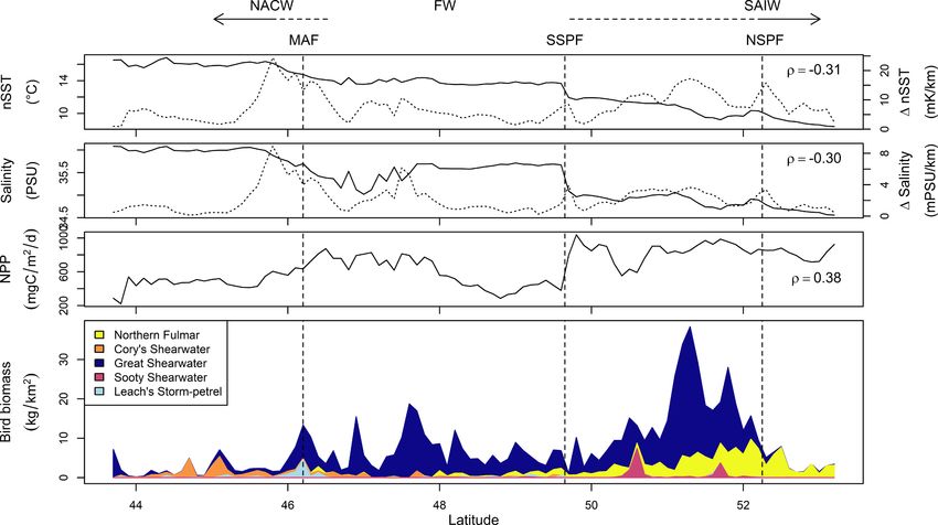
E.D. Wakefield et al. Progress in Oceanography 198 (2021) 102657
Table 1 (Gentemann et al., 2009)) using a local histogram algorithm (Cayula &
Potential environmental explanatory covariates considered during selection of Cornillon, 1992) with a minimum SST step of 0.45 ◦ C, and combined the
models of seabird density. Covariates available throughout the study area were fronts over 3 days (Miller et al., 2015). We then smoothed the resulting
considered in global models, while covariates unaffected by cloud were composite front map using a Gaussian filter (σ = 3 pixels) to convert
considered in local inference models. discrete front contours into a continuous metric. In addition, to identify
Phenomenon Covariate Type† Resolution Global Local frontal regions from locally-measured data, we calculated the smoothed
space time gradient of nSST (ΔnSST) by predicting the first derivative of a local
regression model (Loader, 1999) of nSST vs. distance along the transect,
Accessibility‡ 1/distance to R 4x4 (static) (✓) (✓)
nearest colony km specifying a bandwidth of 250 km. Eddy kinetic energy (EKE): Ocean
(α, km) currents, like the NAC, give rise to turbulence in the form of mesoscale
Water mass Sea surface R 1x1 28 d ✓ eddies, jets and waves, which may enhance or suppress primary pro
temperature km duction through the transport of nutrients into or out of the mixed layer
(SST, ◦ C)
Near sea L 3.4 12 m* ✓
or aggregate biota through convergent advection (Falkowski et al.,
surface km* 1991; Gruber et al., 2011). The intensity of turbulence may therefore
temperature affect seabird prey availability (Bertrand et al., 2014; Tew Kai & Marsac,
(nSST, ◦ C) 2010). We quantified mesoscale turbulence using EKE, where
Thermal fronts Square root R 9×9 3d ( )
EKE = 1/2 u2a +v2a and ua and va are the zonal and meridional
✓
front gradient km
(FG, ◦ C/pixel) geostrophic current anomalies. Sea level anomaly (SLA): Mesoscale
Square root L 3.4 12 m* ✓ eddies/meanders may affect seabird distributions by enhancing or
nSST gradient km* suppressing primary production; containing prey assemblages distinct
(ΔnSST, ◦ C/
from surrounding waters; or concentrating planktonic organisms near
km)
Mesoscale Square root R 28 1d ✓ ✓ the surface, especially at eddy margins (McGillicuddy, 2016; Tew Kai &
mixing/ eddy kinetic km Marsac, 2010). We used daily the SLA to indicate the presence of either
aggregation energy (EKE, cold- (negative MSLA) or warm-core (positive SLA) eddies. We obtained
m2/s2)
both daily SLA and geostrophic current data from the Global Ocean
Mesoscale Sea level R 28 1d ✓ ✓
eddies (sign anomaly (SLA, km
Gridded L4 Sea Surface Heights and Derived Variables dataset (spatial
and m) resolution 0.25◦ , ~28 km), downloaded from http://marine.copernicus.
intensity)
eu/ (accessed October 2, 2019). Net primary production (NPP). We
Primary Log net R 9 km 8d ✓
production primary assume that seabird prey abundance increases with NPP via trophic
production cascades (Shaffer et al., 2006; Wakefield et al., 2014). We downloaded 8
(NPP, mg C/ day and monthly NPP data (spatial resolution 1/12◦ , ~9 km), estimated
m2/day)
using a carbon-based production model (Behrenfeld et al., 2005), from
†
R = remotely-sensed, L = measured locally shipboard during the survey. http://sites.science.oregonstate.edu/ocean.productivity/index.php
‡
Only considered for species breeding at the time of the survey (Northern (accessed October 7, 2019). To improve their spread, we log-
Fulmars, Cory’s Shearwaters and Leach’s Storm-petrels).
* transformed NPP and square root transformed EKE and FG prior to
Resolution after averaging over each track segment.
model fitting.
colony (Wakefield et al., 2011). For non-breeding species (GRSH and
3.5. Density modelling
SOSH), we assumed that α was approximately uniform across the study
area. Sea surface temperature (SST): Different water masses are
We had two aims in modelling seabird density: (1) to investigate
characterised by different lower trophic level assemblages (Longhurst,
associations between seabirds and environmental conditions and (2) to
1998) so the distribution of seabirds is hypothesised to vary with water
predict seabird distribution and abundance across the study area. To
mass and therefore SST (Ainley & Boekelheide, 1984; Ballance et al.,
meet aim 1, we first modelled the density of each species as a function of
2006; Hunt, 1997; Hyrenbach et al., 2007; Pakhomov & McQuaid,
remotely-sensed environmental indices, plus, for species breeding at the
1996). We obtained gridded Advanced Very High Resolution Radiom
time of the survey, accessibility (hereafter, global models). In addition,
eter SST data (spatial resolution, 1 km) from the NERC Earth Observa
because SST and NPP estimated via remote sensing are prone to signal
tion Data Acquisition and Analysis Service (NEODAAS). The study area
degradation due to clouds (Becker et al., 2010), we fitted a separate
was frequently obscured by clouds during the cruise, so to avoid missing
density model in which explanatory covariates comprised locally-sensed
data we averaged SST over a 28 day window, centred on the study
nSST and ΔnSST, remotely-sensed indices unaffected by clouds (EKE and
period. We measured the near-surface SST (hereafter, nSST) throughout
SLA), and (when relevant) accessibility (hereafter, the local model).
the cruise (±0.001 ◦ C) using a Sea-Bird SBE 38 Digital Oceanographic
Previous habitat modelling studies suggest that seabird distribution is
Thermometer pump-supplied from an inlet at 5.5 m depth. We also
often poorly explained by environmental covariates alone (Block et al.,
measured salinity (±0.005) using a Sea-Bird SBE45 MicroTSG Ther
2011; e.g., Louzao et al., 2009; Wakefield et al., 2017), for example,
mosalinograph fed by the same supply. However, this was highly
because environmental indices are poor proxies for prey or because
correlated with nSST (Spearman’s ρ = 0.95, p < 0.001), so we do not
seabirds are imperfectly informed about the distribution of their prey
consider salinity further in our analysis. Fronts: Seabirds and their prey
(Grémillet et al., 2008). For the purposes of predicting distribution and
are often more abundant in the vicinity of thermohaline fronts, either
abundance (aim 2), we therefore augmented the global model for each
because elevated nutrient supply at fronts enhances primary production
species by adding smooth of spatial location (see below), referring to the
or because convergent currents associated with fronts cause biota to
result as the spatial smooth model.
aggregate (Bost et al., 2009; Scales et al., 2014). Following Miller et al.
To model bird density, we divided transects into 12 min segments
(2015), we quantified the presence and intensity of fronts as a contin
(equivalent to ~ 3.4 km at a speed of 17 km/h), indexed by j, this length
uous metric, front gradient (FG), defined as the mean front gradient
being chosen to reduce serial autocorrelation whilst retaining sufficient
magnitude, spatially smoothed to produce a continuous distribution
spatial resolution to model habitat relationships (Huettmann & Dia
from discrete contours. In brief, we detected fronts in daily-merged
mond, 2006). Recalling that for NOFU and shearwaters ̂ pf ∕
=̂ p w , we
microwave and infrared SST maps (9 km spatial resolution
specified two simultaneous sets of segments for these taxa, indexed by s,
5
E.D. Wakefield et al. Progress in Oceanography 198 (2021) 102657
one containing in-flight detections (s = 0) and the other on-water de intercept and the state covariate (hereafter, state-only models).
tections (s = 1) (Miller et al., in review). We then modelled counts per We examined correlations among explanatory covariates using cor
segment nj,s as Generalised Linear Models (GLMs) or Generalised Addi relation matrices (Dormann et al., 2013) but following Morrissey and
tive Models (GAMs) with the form Ruxton (2018), we did not automatically exclude candidate explanatory
( ) covariates simply because they were correlated with others. Starting
∑ ( )
[ ]
E ns,j = ̂
p s,j Aj exp β0 + βstate states + fm xjm (1) with all explanatory covariates structured as quadratic terms (Table 1),
m we simplified models by sequentially removing second then first order
polynomials in order of their significance. We assessed model fit and
where β0 is the intercept, βstate estimates the mean difference between conformity to assumptions using quantile–quantile and residual plots
counts of birds on the water and in flight, and fm are either linear or and residual serial autocorrelation using correlograms (Wood, 2017). To
quadratic functions of the environmental assess residual spatial correlation, we fitted GAMs with a bivariate
covariates xj , plus, in the case of the spatial smooth model, a smooth smooth of location to each model’s residuals, reasoning that residuals
of segment location (see Section 3.7). In effect, Eq. (1) treats the data as randomly distributed in space would result in a smooth with zero
arising from two surveys conducted simultaneously (Miller et al., in effective degrees of freedom.
review). While the other terms in the model assume that the spatial
pattern is the same for birds in flight and on the water, the βstate term 3.7. Predicting distribution and abundance
allows the mean density of birds in these behavioural states to differ. The
term ̂p s,j Aj , which enters the model as an offset, is the effective area of For the purposes of predicting distribution and abundance across the
the segment (sensu Miller et al., 2013a), where Aj = wlj , w is the transect study area, we refitted the best global inference model for each species
width (300 m) and lj the segment length. Based on exploratory analysis, with an additional bivariate Duchon spline smooth of segment location
we assumed that nj,s conformed to a negative binomial distribution for with a maximum basis dimension of 30. Using these models, we pre
all species. We fitted models using the R package dsm (Miller et al., dicted the abundance of each species (birds on the water, plus birds in
2021). We took a similar approach for LHSP but specified a single set of flight) across a Lambert Azimuthal Equal Area grid (cell size 4 × 4 km)
segments, containing both birds detected in flight and on the water, and encompassing, and centred on, the study area. COSH, GRSH and SOSH
modified equation (1) by removing βstate . all dive frequently (Bonnet-Lebrun et al., 2020; Paiva et al., 2010a;
Ronconi et al., 2010b). In order to account for the resulting availability
bias (Buckland et al., 2015) for these species, we multiplied their pre
3.6. Model selection and validation dicted abundance by the inverse of the mean proportion of time they
spend at the surface during daylight hours (Winiarski et al., 2014),
Selecting species distribution models from a set of candidates that estimated using the TDR data (Supplementary Methods). Although
includes very complex or ecologically unrealistic models can result final Leach’s petrels and NOFU are capable of diving, they do so infrequently
models that predict poorly in unsampled regions (Bell & Schlaepfer, (Garthe & Furness, 2001; Ortega-Jiménez et al., 2009), so following
2016). We used the following strategies to avoid this. Firstly, we defined previous studies (e.g. Waggitt et al., 2020), we assumed that availability
candidate models based on prior understanding of how environmental bias is negligible for these species. We estimated uncertainty in pre
phenomena (measured by available proxies, such as SST), might affect dicted abundance by posterior simulation, using a technique adapted
seabird distribution. Secondly, we assumed that, on the scale of the from Wood (2017; Section 7.2.6). In brief, we randomly drew model
linear predictor, associations between seabird density and environ parameters from their estimated multivariate normal distribution,
mental covariates could be adequately approximated by linear or second propagating uncertainty due to both the detection function and count
order polynomial terms. Thirdly, we reduced model complexity by model following Bravington et al. (2021). We then predicted the abun
backwards selection based on spatial cross-validation, assuming that a dance in each cell and across the study area, if relevant, applying an
good model should predict accurately in areas of space not included in availability bias correction randomly drawn from its posterior distri
the training data set (Roberts et al., 2017; Wenger & Olden, 2012). bution. We repeated this process 1000 times and then calculated the cell-
Finally, we compared predicted density to patterns of spatial usage level and overall means and their corresponding coefficients of variation
observed independently via tracking. and 95% confidence intervals. To compare our results to Davies et al.
Starting with the terms shown in Table 1, we built the global and (2021)’s tracking-based estimates of adult abundance, we also used this
local inference models by backwards selection based on cross-validation method to predict abundance in the NACES pMPA, multiplying this by
in a similar manner to Roberts et al. (2017). We divided the study area the assumed proportion of adults in the study area. For NOFU and LHSP,
into nine blocks (Fig. A1), this number being chosen to provide units the proportion of adults was inferred from our moult observations. For
that both represented the range of environmental conditions across the the remaining species, it was assumed, based on published estimates
study area and held similar amounts of survey data. We then fitted the (Brooke, 2004a; Carneiro et al., 2020), to be ~50%. We converted
model under consideration to data from eight of the blocks, predicted for observed and predicted abundances to biomasses using estimates of
the remaining block and calculated the logarithmic score of these pre mean body mass reported by Brooke (2004a).
dictions. The logarithmic score is the negative log of the probability of
obtaining a given count, and has been advocated for the selection of 3.8. Geolocator processing and comparison with model predictions
count models due to its simplicity and propriety (Czado et al., 2009). We
repeated this process for all blocks and then calculated the mean loga We used the probGLS package to estimate two locations/bird/day
rithmic score S, across spatial blocks as: from geolocator data, modifying the methods described by Merkel et al.
1∑9 1 ∑mi (2016) for trans-equatorial migrants (see Supplementary Methods).
S= − logP− i (xmi ) (2) Median location errors using this method are ~185 and 145 km during
9 im j
the equinoxes and solstices, respectively (Merkel et al., 2016). We
where blocks are indexed by i and there are mi observations within each compared the model-predicted spatial distribution of each species to the
block, indexed by j. P− i is the probability mass function for the model distribution of birds in the study area estimated from tracking data
fitted to all but block i. S decreases as the predicted counts approach following Carroll et al. (2019). In brief, we estimated the utilisation
their observed counterparts so, during model selection, we accepted a distribution (UD) of each tracked bird using kernel density analysis,
potential model simplification if it resulted in no increase in S. For implemented in the adehabitatHR package (Calenge, 2006), specifying a
comparison, we also fitted a model for each species containing only the fixed smoothing parameter of 75 km and the grid described in Section
6
E.D. Wakefield et al. Progress in Oceanography 198 (2021) 102657
3.7. We then averaged UDs across birds. In order to provide sufficient 2018 (see Section 3.2). We quantified the similarity between the model-
data to resolve distribution patterns, we calculated UDs using bird lo predicted distributions and the tracking-based UDs by first cropping the
cations recorded during the seabird survey period ± 20 days. COSH UDs latter to the study area and then normalising each to sum to unity. We
were necessarily estimated using data from the equivalent period in then calculated the Bhattacharya affinity, which ranges from 0 (no co-
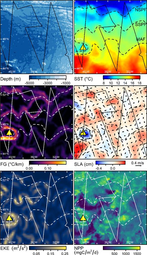
Fig. 2. Environmental conditions in the study
area during the survey (see Table 1 for defini
tions). The solid line indicates the cruise track
and the dashed lines the 10.5, 13 and 14.75 ◦ C
SST isotherms delineating the approximate loca
tions of the North Subpolar Front (NSPF), South
Subpolar Front (SSPF) and Mid-Atlantic Front
(MAF), respectively. The yellow triangle indicates
the centre of the cold-core eddy mentioned in the
text. Geostrophic current anomalies are super
imposed on SLA. (For interpretation of the refer
ences to colour in this figure legend, the reader is
referred to the web version of this article.)
7E.D. Wakefield et al. Progress in Oceanography 198 (2021) 102657
occurrence) to 1 (identical distributions), between these two matrices identified to species. Most abundant were GRSH (64.6 % of in-transect
(Fieberg & Kochanny, 2005). sightings), followed by NOFU (22.0 %), COSH (7.1 %), SOSH (2.4 %)
and Manx shearwaters (Puffinus puffinus, 0.4 %). LHSP were also
3.9. Species associations detected relatively frequently (2.8 %) but a small proportion of
Hydrobatidae/Oceanitidae sightings (3.5 % of 141 birds) were not
To establish which species typically co-occurred with one another at identifiable to species. Based on size, the majority were suspected to be
fine scales (~4 km), we calculated the Chao-Jaccard similarity index Wilson’s storm-petrels so these records were not included among the
(Chao et al., 2005) between per-species segment counts and linked data used to model LHSP density.
similar species using Ward clustering (Kauffman & Rousseeuw, 2005). At the meso- to macroscale (100s–1000s km), mean avian biomass
We restricted this analysis to species detected in at least 20 segments. increased with latitude and NPP and decreased with nSST and salinity,
peaking between the NSPF and SSPF (Fig. 3). At the mesoscale (10
4. Results s–100 s of km), two notable seabird aggregations occurred - one in the
NE of the study area, between the SSPF and NSPF (cf. Fig. A2 and Fig. 2)
4.1. Survey effort and environmental conditions and another smaller one 350 km east of the Flemish Cap, associated with
the cold-core eddy described above. Cluster analysis indicated that at
The seabird survey covered 3265 km in 192 h. Beaufort wind force coarse scales (1–10 km) and above, the more common species tended to
averaged 4.5 ± 1.6 and wave height 1.7 ± 0.8 m during survey bouts. co-occur in two groups (Fig. 4), the first comprising GRSH, NOFU and
Visibility averaged 9 ± 7 km but fell as low as 300 m at times in the west SOSH, which were most abundant north of the SSPF (Fig. 3), and the
of the study area due to fog. SST ranged from ~18 ◦ C in the south of the second COSH and LHSP, which were mostly confined to the south. Arctic
study area to 8 ◦ C in the north (Fig. 2) and the mean latitudes of the terns (Sterna paradisaea) and Manx shearwaters, occurred throughout
MAF, SSPF and NSPF were 46◦ 12′ , 49◦ 39′ and 52◦ 15′ N, respectively the area. Taxa occurring in smaller numbers included all three jaeger
(Fig. 3). Multiple mesoscale eddies were crossed, including an intense spp. (Stercorarius longicaudus, S. parasiticus and S. pomarinus), recorded
cold-core ring (diameter ~ 140 km) centred at 46◦ 5′ N, 40◦ 30′ W, ~340 throughout the study area, and Catharacta skuas, recorded almost
km ESE of the Flemish Cap (Fig. 2). NPP was markedly higher north of exclusively south of the SSPF (Fig. A2). All of the Catharacta spp. (7 of 19
the SSPF than to the south (means 815 vs. 590 mg C/m2/day; Fig. 3) but birds) that could be positively identified (following Newell et al., 2013)
isolated patches of high NPP also occurred south of this, associated with were South Polar Skuas (C. maccormicki).
negative SLAs, including the eddy just mentioned (Fig. 2). Of those birds whose moult could be assessed, 59 % of 334 NOFU, 3
% of 237 COSH, 70 % of 894 GRSH and 50 % of 10 SOSH were in active
primary moult. The likelihood of primary moult among NOFU increased
4.2. Observed distribution and characteristics of seabirds
significantly with distance from the nearest colony (Fig. A3; binomial
GLM Z1, 332 = 3.15, p = 0.002). Of the 1201 NOFU for which colour
We recorded eighteen species of seabird during the survey (Table 2),
phase was assessed, 94 % were LL, 4 % L, and 2 % D. Of those for which
totalling 7464 individuals. Of these, 4692 were sighted in transect, the
moult was also assessed (n = 307), a significantly higher proportion (25
vast majority (96.5 %) being medium-sized petrels, all of which were
Fig. 3. Surface hydrography and observed biomass (corrected for imperfect detection) of the five most abundant seabird species averaged by latitude over the survey
track. Near-sea surface temperature (nSST) and salinity were measured ship-board at 5 m depth and net primary production (NPP) was estimated from remotely-
sensed data (Behrenfeld et al., 2005). ρ indicates Pearson’s correlation between these indices and bird biomass. nSST and salinity gradients (dotted lines) were
calculated prior to averaging by latitude (see Section 3.4). Dashed vertical lines indicate the approximate mean latitudes of the major fronts defined in Fig. 2 and
arrows the mean extents of North Atlantic Central Water (NACW), Frontal Water (FW) and Sub-Arctic Intermediate Water (SAIW).
8E.D. Wakefield et al. Progress in Oceanography 198 (2021) 102657
Table 2
Number of birds recorded in the study area in June 2017 and groups sizes.
Taxon Total Birds in % in Median group
birds transect1 groups2 size (LQ-UQ3,
max.)
Northern Fulmar 1970 1034 44 2 (2–3; 9)
Fulmarus glacialis
dark petrel sp. 1 0
Cory’s Shearwater 741 331 44 3 (2–5; 28)
Calonectris borealis
Great Shearwater 4203 3029 76 3 (2–6; 46)
Ardenna gravis
Sooty Shearwater 178 114 64 4 (3–5; 30)
A. grisea
small shearwater sp. 1 0
Puffinus sp.
Manx Shearwater 30 19 11 2 (2–2; 2)
P. puffinus Fig. 4. Chao-Jaccard index showing similarity in observed abundance of the
Bulwer’s Petrel* 1 0 commonest species (those present in ≥ 20 segments) at the scale of survey
Bulweira bulwerii segments (~4km). Species with similar abundance patterns were linked by
Wilson’s Storm-petrel* 9 6 33 2 (2–2; 2) Ward clustering.
Oceanites oceanicus
storm petrel sp. 20 5 0
Hydrobatidae/ 4.3. Detection functions
Oceanitidae sp.
Leach’s Storm-petrel* 225 130 75 3 (2–3; 45) Slightly more NOFU were detected in the 50 – 100 m distance band,
Oceanodroma
leucorhoa
than in the 0–50 m band. A half-normal model, with scale parameter
Northern Gannet Morus 3 0 covariates visibility (continuous, km) and precipitation (true/false), was
bassanus selected based on AIC (Table A4, Fig. A5). Precipitation (especially fog)
skua sp. Stercorarius/ 4 1 0 may have affected the detectability of NOFU more than other species
Catharacta sp.
due to their relatively light colouration. However, compared to the other
jaeger sp. Stercorarius sp. 8 4 50 2 (2–2; 2)
Pomarine Jaeger* S 4 1 0 taxa, the detectability of NOFU (mean probability of detection ̂ pw =
pomarinus 0.51) varied relatively little within the range of environmental condi
Arctic Jaeger* 4 0 tions experienced during the survey (Fig. A5). A half-normal model with
S. parasiticus scale parameter covariates for visibility and Beaufort wind speed best
Long-tailed Jaeger 4 1 0
S. longicaudus
described the probability of detecting GRSH, SOSH and COSH on the
large skua sp. Catharacta 12 3 0 water (̂p w = 0.48). A half-normal model, with a scale parameter varying
sp. with wind speed, best described the probability of detecting LHSP on-
South Polar Skua 7 3 0 water and in-flight (̂ p w = 0.51). Variation in this probability was rela
C. maccormicki
Atlantic Puffin Fratercula 1 1 0
tively large over the range of wind speeds experienced during the survey
arctica (Fig. A5), presumably because LHSP are harder to detect as sea condi
Common Guillemot Uria 1 0 tions deteriorate than the other species considered.
aalge
Brunnich’s Guillemot 1 1 0
U. lomvia 4.4. Habitat associations
Common/Arctic Tern 10 1 0
Sterna hirundo/ Correlations among candidate explanatory environmental covariates
paradisaea were < 0.7 (Table A5), with the exception that SST was positively
Arctic Tern S. paradisaea 24 6 33 2 (2–2; 2)
Great Black-backed 1 1 0
correlated with accessibility for COSH (ρ = 0.83, p < 0.001). However,
Gull** Larus marinus accessibility was rejected during model selection (Fig. 5, Fig. A6). There
1 was no consistent pattern in whether the global or local inference
In transect refers to birds sighted on the water, within the 300 m wide survey
models best described density for each species (Table 3).
strip or in flight in a 300 × 300 m box during instantaneous ‘snapshots’, which
occurred every 300 m (see Methods).
For NOFU, both the global and local inference models indicated
2
A group is defined here as ≥ 2 birds recorded in transect in a one-minute similar environmental associations (Fig. 5). Density initially rose with
interval. SSTs and nSSTs, peaked around 10–12 ◦ C and declined sharply above ~
3
Lower and upper quartiles. 13 ◦ C, indicating that this species associates principally with SAIW and
*
Species not detected in the study area in April-June via tracking data ana FW. In addition, NOFU were positively associated with fronts and
lysed by Davies et al. (2021). negatively associated with EKE. The local model, which had the best
**
Species not reported in the study area by previous at-sea or tracking studies predictive performance (Table 3) and lowest residual autocorrelation
(Bennison and Jessopp, 2015; Boertmann, 2011; Godø, 2004; Priede, 2007; Skov (Fig. A7), additionally suggested that NOFU density increased with SLA.
et al., 1994; Davies et al., 2021). The global and local inference models for COSH had very similar
structures, but the latter predicted more accurately and exhibited lower
of 27) of darker NOFU (i.e. L or D) were in active primary moult than LL residual autocorrelation. Both indicated a positive association between
birds (154 of 280; Fisher’s exact test, p < 0.001). There was no signif COSH density and SST (Fig. 5), the latter indicating highest densities in
icant linear trend in the occurrence of darker phase NOFU with latitude NACW. In addition, density increased with absolute SLA, with highest
(binomial GLM Z1, 1200 = 0.87, p = 0.382) but their proportion was COSH densities occurring coinciding with negative SLAs. The local
marginally higher north of 51.5◦ N (χ21, 1065 = 3.94, p = 0.047; Fig. A4). model also indicated a weak negative association with EKE. Both GRSH
Based on plumage, the vast majority of Northern Gannets (Morus bas inference models performed poorly compared either to the GRSH state-
sanus), jaegers and Arctic Terns in the study area were immatures only model or the inference models for the other species (Table 3).
(Table A3). Moreover, the global and local GRSH inference models both exhibited
9E.D. Wakefield et al. Progress in Oceanography 198 (2021) 102657
Fig. 5. Partial associations between bird density and environmental indices, predicted by the global and local inference models (see Fig. A6 for associations on the
scale of the linear predictor). Global models contain only remotely-sensed environmental covariates, whereas local models contain remotely-sensed covariates
unaffected by cloud and locally-sensed environmental covariates (see Table 1 for definitions). Dashed vertical lines show the approximate latitudes of the major
fronts defined in Fig. 2.
relatively high residual autocorrelation (Fig. A7). The former indicated a 4.5. Predicted distribution and abundance
positive association between GRSH and FG, whereas the latter implied a
negative association with nSST (Fig. 5), with density being highest in For all species, inclusion of a spatial smooth reduced residual serial
SAIW/FW. For SOSH, the global inference model performed better than and spatial autocorrelation markedly (Fig. A7). The mean proportion of
the local model (Table 3, Fig. A7). Both indicated an association with time TDR-equipped shearwaters spent diving during daytime varied
cooler temperatures (SAIW/FW) but the remaining covariates were seasonally and between species (Fig. A8). During the survey period,
inconsistent between models: The global model additionally indicated a COSH, GRSH and SOSH spent on average 0.13 (95% CI 0.08–0.23), 0.24
positive association with FG and a negative association with NPP, while (0.07–0.81) and 1.50 (1.01–2.23) % of their time diving, respectively, so
the local model indicated a positive association with SLA. The local and availability bias had little effect on our abundance estimates (Fig. A9).
global models for LHSP were very similar to one another but the latter GRSH were predicted to be the most abundant species in the study
had the better predictive performance (Table 3, Fig. A7). Both indicated area (~3.9 million individuals, Table 4) and their predicted density
a positive association with SST and especially NACW (Fig. 5). highest along its SW/NE axis, peaking in the NE (Fig. 6). Eighteen out of
10You can also read