ICES WGBIODIV REPORT 2018 - ECOSYSTEM PROCESSES AND DYNAMICS STEERING GROUP Report of the Working Group on Biodiversity Science (WGBIODIV)
←
→
Page content transcription
If your browser does not render page correctly, please read the page content below

ICES WGBIODIV REPORT 2018
       E COSYSTEM P ROCESSES   AND   D YNAMICS S TEERING G ROUP

                                 ICES CM 2018/EPDSG:01

                                                 R EF . SCICOM

      Report of the Working Group on
      Biodiversity Science (WGBIODIV)

                                5-9 February 2018

ICES Headquarters, Copenhagen, Denmark
International Council for the Exploration of the Sea
Conseil International pour l’Exploration de la Mer
H. C. Andersens Boulevard 44–46
DK-1553 Copenhagen V
Denmark
Telephone (+45) 33 38 67 00
Telefax (+45) 33 93 42 15
www.ices.dk
info@ices.dk

Recommended format for purposes of citation:

ICES. 2018. Report of the Working Group on Biodiversity Science (WGBIODIV), 5–9
February 2018, ICES Headquarters, Copenhagen, Denmark. ICES CM
2018/EPDSG:01. 82 pp.

For permission to reproduce material from this publication, please apply to the Gen-
eral Secretary.

The document is a report of an Expert Group under the auspices of the International
Council for the Exploration of the Sea and does not necessarily represent the views of
the Council.

© 2018 International Council for the Exploration of the Sea
ICES WGBIODIV REPORT 2018                                                                                                                         | i

C o nten ts

       Executive summary ................................................................................................................ 3

       1      Administrative details .................................................................................................. 4

       2      Terms of Reference ........................................................................................................ 4

       3      Summary of Work plan ................................................................................................ 5

       4      Summary of Achievements of the WG during 3-year term ................................... 5

       5      Final report on ToRs, workplan and Science Implementation Plan .................... 6
              5.1      Protocol on the development of theoretical concepts for
                       biodiversity indicators (ToR1a, Deliverable 1) ................................................. 6
                        5.1.1 Introduction .............................................................................................. 6
                        5.1.2 Background ............................................................................................... 7
                        5.1.3 A step-by-step approach to theory-based indicator
                              conception ................................................................................................. 9
                        5.1.4 Case studies ............................................................................................ 15
                        5.1.5 Conclusions............................................................................................. 19
                        5.1.6 References ............................................................................................... 19
              5.2      Standardizing sampling design and analysis to obtain unbiased
                       estimates of species diversity (ToR1b, Deliverable 2) .................................... 24
                        5.2.1 Introduction ............................................................................................ 24
                        5.2.2 Species area relationship (SAR) and species accumulation
                              curve (SAC)............................................................................................. 26
                        5.2.3 Case studies ............................................................................................ 28
                        5.2.4 References ............................................................................................... 49
              5.3      Development of a Benthic Community Physical Disturbance
                       Indicator ............................................................................................................... 51
                        5.3.1      Introduction ............................................................................................ 51
                        5.3.2      Policy rationale ....................................................................................... 52
                        5.3.3      Scientific rationale .................................................................................. 53
                        5.3.4      Constructing a traits-based indicator .................................................. 55
                        5.3.5      Application of the indicator to two different case studies ............... 57
                        5.3.6      Discussion ............................................................................................... 68
                        5.3.7      The future................................................................................................ 70
                        5.3.8      References ............................................................................................... 70

       6      Cooperation .................................................................................................................. 72

       7      Summary of Working Group self-evaluation and conclusions .......................... 72

       Annex 1: Lists of participants ............................................................................................. 73

       Annex 2: Recommendations ............................................................................................... 76

       Annex 3: WGBIODIV draft resolution 2019–2021 .......................................................... 77
ii |                                                                                   ICES WGBIODIV REPORT 2018

       Annex 4: WGBIODIV self-evaluation .............................................................................. 80
ICES WGBIODIV REPORT 2018                                                                      | 3

Executive summary

       The ICES Working Group on Biodiversity Science (WGBIODIV), chaired by W. Nikolaus
       Probst, Germany, and Oscar Boss, the Netherlands, has held three annual meetings in
       2016–2018.
       WGBIODIV worked on theoretical concepts of diversity indicators along several lines.
       The quantification of changes in biodiversity is often considered central to the assess-
       ments of human impacts on marine ecosystems, but this quantification has been proven
       as an exceptionally difficult task. WGBIODIV developed a generic protocol on how indi-
       cators need to be underpinned conceptually to provide indicators of biodiversity with
       meaningful assessment targets. WGBIODIV also analysed the impacts of sampling de-
       sign on estimates of species diversity. And finally, WGBIODIV developed a trait-based
       sensitivity indicator for benthic community in response to bottom trawling.
       The generic protocol on indicator development identified seven steps that should be con-
       sidered when developing indicators for environmental status assessments. Especially the
       development of a theoretical indicator framework is crucial, because it helps to develop
       meaningful assessment benchmarks. At the moment, many status indicators used for
       environmental status assessments by the regional seas conventions are missing this
       framework or using a non-quantitative theoretical background, which impairs the defini-
       tion of quantitative assessment targets.
       The influence of sampling design on estimates of diversity metrics was analysed in four
       different case studies: (i) comparing different methods for calculating species accumula-
       tion curves, (ii) analysing the influence of sampling size on North Sea fish species, (iii)
       analysing the impact of spatial resolution on plankton indicators and (iv) analysing the
       relationship between sampling effort and species number in soft bottom benthos. These
       case studies show that patterns of diversity strongly depend on the sampling scheme,
       which therefore requires careful consideration to provide the adequate data to feed into
       assessments.
       WGBIODIV used traits-based data on benthic invertebrate communities to develop a
       community physical disturbance indicator. This indicator combines functional character-
       istics of benthic species, including their sensitivity to physical perturbations (i.e. their
       response through injury or death) and their recoverability (i.e. the self-sustainability of a
       population when damaged and/or its recolonization potential following mass mortality).
       The behaviour and performance of the indicator was examined using two independent
       case studies from the Dutch EEZ and the Bay of Biscay. Future investigations of
       WGBIODIV will focus on comparison of the distribution of indicator values between
       different geographical areas and, for some locations, over time. We will use the indicator
       to test hypotheses on the relationship between trawl effects and function of benthic
       communities.
4 |                                                                                 ICES WGBIODIV REPORT 2018

      1        Administrative details

               Working Group name

               Working Group on Biodiversity Science (WGBIODIV)

               Year of Appointment within current cycle

               2016

               Reporting year within current cycle (1, 2 or 3)

               3

               Chair(s)

               W. Nikolaus Probst, Germany
               Oscar Bos, the Netherlands

               Meeting dates and venues

               8–12 February 2016, San Sebastian, Spain (15 participants)
               6–10 February 2017, Venice, Italy (19 participants)
               11–12 February 2018, Copenhagen, Denmark (12 participants)

      2        Terms of Reference

ToR   Description                                       Background                     Science    Duration Expected
                                                                                       Plan                Deliverables
                                                                                       priorities
                                                                                       addressed

a      Develop the use of biodiversity metrics (e.g.     Initiatives to revise the EC 1, 5, 9, 11, 3 years   1. Protocol on the
       species richness and species evenness indi-       Decision of 2010 suggest that 12,                   development of
       ces) to inform on the status of ecosystem         metrics for the ecosystem level 13,16,18,           theoretical con-
       components at the community level (fish,          of biodiversity may simply not                      cepts of biodiver-
       mammals, seabirds, plankton, epi-benthos,         be possible given the current                       sity    indicators
       macro-algae) to support implementation of         level of scientific knowledge.                      (2016/2017).
       ecosystem-based management. This task             Instead metrics at community
                                                                                                             2.     Combined
       encompasses:                                      level may be achievable, and
                                                                                                             analysis and re-
                                                         indeed community level met-
       1a. Establish a sound theoretical basis relat-                                                        view on impacts
                                                         rics represent the logical pro-
       ing variation in biodiversity metric values                                                           of sampling size
                                                         gression from species level
       to changes in anthropogenic pressure on                                                               on performance
                                                         and habitat level in that com-
       marine communities (e.g. incorporating                                                                of    biodiversity
                                                         munities represent the collec-
       components of community size and trophic                                                              metrics    (2016–
                                                         tion of species that occupy a
       structure into the derivation of biodiversity                                                         2018).
                                                         habitat. In applying criteria to
       metrics, taking account of linkage to habitat
                                                         assess the performance of dif-                      3. Analysis on
       types and consideration of spatial pattern).
                                                         ferent community-level met-                         aggregating bio-
       Update: ToR1a may require further work            rics,    metrics   of   species                     diversity indica-
       beyond next years’ meeting and may extend         diversity have routinely per-                       tors at different
       into in the next term (2018–2020), as the         formed below par. A major                           levels   (species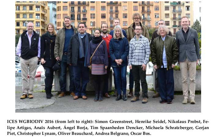
ICES WGBIODIV REPORT 2018                                                                                        | 5

 development of indicator concepts is time        shortcoming in their perfor-                        group, communi-
 consuming.                                       mance has been the lack of a                        ty,    ecosystem)
                                                  sound and well understood                           (2017/2018).
 1b. Explore the issue of sampling size de-
                                                  theoretical basis to explain the
 pendence to derive a robust protocol for                                                             4. Quality as-
                                                  relationship between pressure
 calculating biodiversity metrics so that their                                                       sessment of in-
                                                  and state. Without this under-
 sensitivity to underlying drivers is maxim-                                                          vestigated
                                                  standing, it has always been
 ized, and the ‘noise’ associated with sam-                                                           biodiversity indi-
                                                  assumed that it would be dif-
 pling effects is minimized (e.g. procedures                                                          cators according
                                                  ficult to formulate sound reli-
 for sample aggregation, modeling of indi-                                                            to     WGBIODIV
                                                  able scientific advice to
 vidual species distribution to derive point-                                                         criteria (2018).
                                                  support management based on
 diversity estimates).
                                                  observed variation in species                       5. One or more
 1c. Assess the “ecosystem level” assessment      diversity indicators. Conse-                        operational indi-
 of biodiversity by considering how com-          quently the community level                         cators to assess
 munity-level biodiversity metrics might be       indicators that have been used                      biodiversity    at
 aggregated across communities (e.g. inte-        to support EAM initiatives,                         the community
 grated ecosystem assessments of biodiversi-      such as the OSPAR EcoQO                             and eventually
 ty).                                             pilot study and currently to                        the     ecosystem
                                                  fulfil the indicator 1.7.1 role                     level (2018).
 Update: ToR1c may not be addressed dur-          for the MSFD focus on size
 ing the 2016–2018 term as the development        based indicators such as the
 of trait-based indicators will not be com-       large fish indicator. Given the
 pleted until 2018.                               species diversity indicators
 1d. Apply the WGBIODIV quality criteria to       would appears to be the most
 assess the performance of state indicators to    obvious candidates for metrics
 assess the performance of any biodiversity       to fulfil the community-level
 indicators proposed and developed by             indicator role in D1, the
 WGBIODIV to show whether previous                maintenance of biological di-
 weaknesses in such metrics have been ad-         versity, the time is clearly ripe
 dressed.                                         for the theoretical shortcom-
                                                  ings in these indicators to be
 Update: ToR1d may have to be addressed in        addressed so that they can be
 the next term (2018–2020) as the develop-        used to monitor change in
 ment of the new WGBIODIV biodiversity            biodiversity within marine
 indicators may not by finalised in 2018.         communities.

3        Summary of Work plan

             Year 1             Develop theoretical background for several indicators of diversity; establish
                                protocol on indicator development
             Year 2             Calculate biodiverstiy metrics using reference data, provide overview and
                                comparision of outcomes
             Year 3             Evaluate biodiversity indicators according to WGBIODIV indicator quality
                                criteria

4        Summary of Achievements of the WG during 3-year term

         In 2015, WGBIODIV chaired a theme session at the ICES Annual Science Conference on
         measuring and assessing biodiversity. The theme session hosted 18 oral presentations
         and three posters.
6 |                                                                       ICES WGBIODIV REPORT 2018

      Members of WGBIODIV published two papers during the 2016–2018 reporting cycle:
          •    Probst, W. N., Lynam, C. P. 2016. Aggregated assessment results depend on ag-
               gregation method and framework structure - a case study within the European
               Marine Strategy Framework Directive. Ecological Indicators, 61: 871–881.
          •    Rambo, H., Stelzenmueller, V., Greenstreet, S.P.R., Moellmann, C. 2017. Mapping
               fish community biodiversity for European marine policy requirements. ICES
               Journal of Marine Sciences, 74: 2223–2238.
      Deliverable 3 could not be achieved as only one indicator on benthic communities be-
      came developed. The aggregation of indicators of different ecosystem components was
      thus not possible. To date it remains open when and how WGBIODIV will be able to
      address this deliverable.
      Deliverable 4 could not be achieved, as none of the envisioned indicators could be devel-
      oped so far as to make it operational. Thus, an evaluation according to the WGBIODIV
      indicator quality criteria was not possible, but may be achievable in the next three-year
      working cycle.

5     Final report on ToRs, workplan and Science Implementation Plan

5.1   Protocol on the development of theoretical concepts for biodiversity
      indicators (ToR1a, Deliverable 1)

      Deliverable 1: Protocol on the development of theoretical concepts of biodiversity indicators
      (2016/2017)

      5.1.1    Introduction

      The lack of fully comprehended pressure-state relationships based on classical biodiversi-
      ty metrics led WGBIODIV to devise ToR1a: “Establish a sound theoretical basis relating
      variation in biodiversity metric values to changes in anthropogenic pressure on marine
      communities (e.g. incorporating components of community size and trophic structure
      into the derivation of biodiversity metrics, taking account of linkage to habitat types and
      consideration of spatial pattern).”
      During the three-year working period from 2016 to 2018 several theoretical concepts for
      functional biodiversity indicators were introduced and explored (see Chapter 5.3). This
      chapter ‘Protocol on the development of theoretical concepts of biodiversity indicators
      (2016/2017)’ aims to distil generic principles for developing theory-based biodiversity
      indicators.
      The focus of this protocol will be on the development of community indicators, as single-
      species indicators may require less theoretical understanding as they are in many cases
      linked more directly to human pressures. However, most parts of this protocol should be
      generically applicable to single-species indicators alike.
      The steps are:
      Step 1: Identify relevant features
      Step 2: Develop theoretical underpinning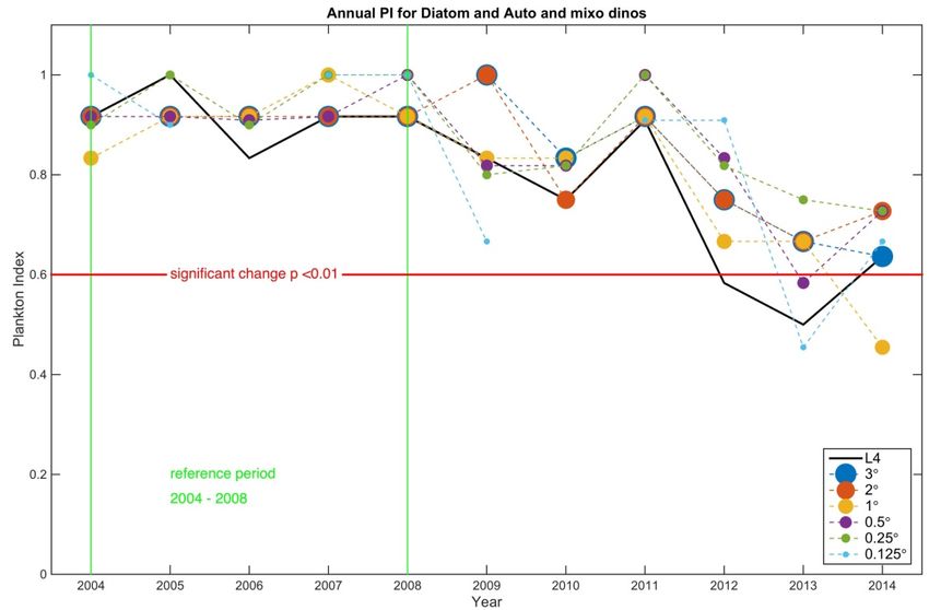
ICES WGBIODIV REPORT 2018                                                                                  | 7

       Step 3: Develop the indicator
       Step 4: Establish pressure-state relationship(s) (for operational indicator)
       Step 5: Obtain “adequate status” targets (for operational indicators)
       Step 6: Perform indicator evaluation
       Step 7: Apply indicator concept to field data

       5.1.2    Background

       Ecological indicators are essential in ecosystem assessments

       The increasing awareness of broad scale impacts of human activities on the marine envi-
       ronment instigated the implementation of ecosystem based approaches to marine man-
       agement, either within single management sectors (Link, 2010; Belgrano and Fowler,
       2011; Hilborn, 2011; Link and Browman, 2014) or across the full range of managed hu-
       man activities (Arkema et al., 2006; Leslie and McLeod, 2007; ICES, 2015). The implemen-
       tation of ecosystem based management approaches is commonly associated with either
       integrating multiple single elements (Ojaveer and Eero, 2011; Probst and Lynam, 2016) or
       full integrated ecosystem-level assessments (IEA); (Toth and Hizsnyik, 1998; Levin et al.,
       2009; Möllmann et al., 2014). In either case, integrated assessments are based on indicators
       (Garcia et al., 2000; Jennings, 2005). Ecological indicators are intended to capture or repre-
       sent relevant features of the ecosystem which representatively inform on wider aspects of
       ecosystem health thereby guiding management agencies towards targeted action (OECD,
       1993; Helsenfeld and Enserink, 2008).
       The implementation of ecosystem-based approaches to marine management has initiated
       intensive research and development programmes on environmental and ecological indi-
       cators (see for example Mace and Baillie, 2007; Helsenfeld and Enserink, 2008; EU-COM,
       2010; Shin et al., 2010; HELCOM, 2013). In fact, the number of suggested indicators has
       become overwhelmingly large, sometimes leading to redundancy in their content and
       meaning (Greenstreet et al., 2012a; Shephard et al., 2012). Thus, technical frameworks for
       selecting indicators based on quality criteria have been proposed and applied (Rice and
       Rochet, 2005; ICES, 2012; ICES, 2013; Probst et al., 2014; Queirós et al., 2016). These
       frameworks define evaluation criteria to indicators addressing (amongst others) the data
       quality, sensitivity and responsiveness towards changes in anthropogenic pressures,
       comprehensibility, theoretical underpinning and (cost) effectiveness.
       In this chapter, we focus on two types of indicators: ‘operational indicators’ link human
       disturbances (pressure) to the state of an ecosystem component and ‘surveillance indica-
       tors’, which are used for surveillance of single ecosystem components without a clear
       assessment target and direct link to specified pressures (Shephard et al., 2015). Surveil-
       lance indicators are not directly linked to specific pressures, but aim to warn manage-
       ment if the ecosystem is leaving previously known boundaries

       The lack of theoretical underpinning leads to unclear status targets: The case of fish indicators

       Classical fish biodiversity indicator metrics (species richness or evenness) fail to score
       well with regards to sensitivity and responsiveness towards human disturbances (Green-
       street, 2008). This is in large proportion due to the circumstance that the relationship
8 |                                                                ICES WGBIODIV REPORT 2018

      between human pressures and biodiversity indices, representing the ecological state, is
      often poorly understood (Rice, 2000). A study by Piet and Jennings (2005) revealed that
      several biodiversity indicators (e.g. Hill’s diversity indices) did not show a consistent
      relationship with fishing intensity and concluded that a better theoretical understanding
      of the response of biodiversity metrics to anthropogenic pressures is necessary.
      To address this problem, recent fish biodiversity indicators were based on the size-
      composition of communities, where marine communities’ biotic interactions are consid-
      ered to be driven by size-structure rather than by taxonomic distinction (Daan et al., 2005;
      Greenstreet et al., 2011). A prominent example for such a size-based biodiversity indicator
      is the Large Fish Indicator (LFI), which assesses the ratio between the biomass of small
      and large fish within a community (Greenstreet et al., 2011; Shephard et al., 2011). How-
      ever, even for indicators such as the LFI, unexpected patterns in the pressure-state rela-
      tionship emerged i.e. that the responsiveness (the time it takes for a state indicator to
      react to changes in pressure) of the LFI to fishing intensity was much longer than previ-
      ously assumed (Fung et al., 2013). This long-lagged responsiveness indicated that the
      initial theoretical concept of the LFI was complicated by trophic cascades within the fish
      community and that a deeper theoretical understanding of fishing impacts on fish com-
      munities may still be necessary. An equivalent type of species diversity indicator to the
      LFI does not currently exist for benthic communities. The majority of existing benthic
      diversity indicators are based on species abundance or biomass (e.g. the OSPAR common
      indicator “BH2 - Condition of benthic habitat defining communities (Multi-Metric Indi-
      ces)”) and thus knowledge of pressure-state relationships between benthic communities
      and anthropogenic impacts is increasingly necessary to support the development of these
      indices.
      The lack of a clear, unambiguous understanding of theoretical concepts underlying eco-
      logical indicators can lead to difficulties in establishing assessment baselines for good
      environmental status (GES). Currently, many indicators are missing assessment targets
      that have been derived from theory. Instead assessment targets are usually based on his-
      torical evidence (Greenstreet et al., 2011; Fock, 2014). In the lack of such historical evi-
      dence, time-series based approaches are suggested (Rochet et al., 2010; Probst and
      Stelzenmüller, 2015). Both approaches, however, are associated with difficulties. Assess-
      ment targets established from historical evidence may become invalid in a changing en-
      vironment e.g. if the targets become affected by climate change (ICES, 2015). Assessments
      based on time-series analyses do not provide meaningful baselines with regard to the
      true environmental status as they only inform on relative changes.
      A well-established example for an assessment target based on a theoretical principle is
      the maximum sustainable yield (MSY) for exploited fish stocks (Jennings et al., 2001).
      Originally the MSY-concept has been developed by Schaeffer based on the idea of sur-
      plus production (King, 2007). Surplus production describes an increased productivity of
      exploited populations when the population size is reduced (e.g. by fishing). The produc-
      tivity of this population is enhanced because density-dependent inhibitions of growth are
      relieved. The MSY-concept has led to the development of reference points for fisheries
      management. Within the advisory framework of the International Council for the Explo-
      ration of the Sea (ICES) the MSY-principle is currently used to obtain limit values for
      sustainable rates of exploitation (FMSY); (Lassen et al., 2014). The MSY-principle has been
ICES WGBIODIV REPORT 2018 | 9
transferred and adapted to obtain reference points of sustainable impacts for endangered
fish species (Le Quesne and Jennings, 2012) and benthic communities (Fock et al., 2011).
5.1.3 A step-by-step approach to theory-based indicator conception
The following section describes several steps to develop a theoretical concept which can
be used to design biodiversity indicators (Figure 5.1.1). This step-by-step guide focuses
on state indicators which intend to capture aspects of biodiversity within communities of
ecosystem components (e.g. fish, benthos or plankton). It remains to be explored if this
approach is applicable to holistic ecosystem indicators and other types of indicators as
well.
Step 1: Identify relevant features
Ecological indicators are eventually about environmental assessment and hence to be
used in management context. Therefore, it is important to define the relevant features
that the management framework is seeking to address. For example, the MSFD defines
several ecological components and human pressures as relevant for the assessment of
environmental status (see Annex III, Tables 1 & 2) and suggests potential indicators to be
used for these assessments (see 2017/848/EU). However, most of the indicators are de-
scribed only qualitatively and with varying degrees of detail. Hence, it has and still is
taking huge efforts by scientists and political managers to come to terms on which exact
ecological elements and human pressures to assess and how the indicators should be
designed around these elements. Therefore, it is crucial to understand and agree upon
which the relevant ecological features are reflected by the indicator metric and to which
pressure they relate.
Figure 5.1.1. Linkages between anthropogenic disturbance, population dynamic processes, environ-
mental states and biodiversity indicators. The ultimate goal is to derive assessment targets from the
pressure-state relationship (PSR).10 | ICES WGBIODIV REPORT 2018
Step 2: Develop theoretical underpinning
The evaluation of OSPAR biodiversity indicators in 2013 by WGBIODIV revealed that
many indicators scored poorly on the conceptual criterion to be “theoretically sound”
(ICES, 2013). The lack of a theoretical underpinning of these indicators resulted in prob-
lems to define meaningful status targets and thus made the assessment of biodiversity
elements based on these indicators difficult. Furthermore, classical indices of biodiversity
provided ambiguous results with relation to human pressures and hence scored general-
ly badly on evaluations by ICES and OSPAR (Greenstreet, 2008; Greenstreet et al., 2011).
WGBIODIV therefore concluded that it was essential to underlie biodiversity indicators
with a sound theoretical concept that allows to formulate hypotheses on the pressure-
state relationship a priori and allowing for rigorous testing of these hypotheses using
empirical data.
In the following three types of theory-based indicators are described to demonstrate the
way ecological theories can facilitate the design of biodiversity indicators.
Trait-based indicators
Species communities are characterised by the abundance of different species which influ-
ence their composition and diversity (Begon et al., 1996). The abundance of each species
within a community is influenced by abiotic conditions and biotic interactions, which in
turn affect its population dynamics. Population dynamics are driven by processes, name-
ly growth, reproduction and mortality (Jennings et al., 2001), which in turn are depending
on external environmental factors and intrinsic species-specific traits (Figure 5.1.1). The
population dynamics of each species will determine the composition and structure of the
community.
Knowing which traits render members of a community susceptible to specific pressures
allows to build quantitative indices that capture and condense this sensitivity (McGill et
al., 2006; Gravel et al., 2016). An example of such a trait-based indicator can be found in
the concept of the WGBIODIV benthic response indicator (see chapter 5.3 of this report)
or the sensitivity of demersal fish species (Greenstreet et al., 2012b). In each case, biologi-
cal traits (age-at-maturity, maximum length, burrowing depth, fragility, etc.) are com-
bined into an index of sensitivity, which then can be calculated for samples of differing
species compositions and related to influencing factors (Beauchard et al., 2017).
Size-based indicators
Size-based indicators can be considered as a special form of trait-based indicators, as
body size is considered to be the major trait affected by human pressure, e.g. by trawl
fishing (HELCOM, 2017; OSPAR, 2017). A classic example is the OSPAR Large Fish Indi-
cator (LFI), which reflects the proportion of large vs. small fish in the demersal fish com-
munity (Greenstreet et al., 2011; Shephard et al., 2011; Modica et al., 2014). Other examples
are the Typical Length (a size composition indicator, ICES, 2014) and Mean Maximum
Length (a species composition indicator) of fish communities implemented within the
recent OSPAR Intermediate Assessment (OSPAR, 2017). The theoretical underpinning in
relation to pressure is that selective fishing alters the size-structure of fish communities
by reducing the number of large species across the community as well as within single-
species populations (Pauly et al., 1998; Jennings et al., 2002; Probst et al., 2013b).ICES WGBIODIV REPORT 2018 | 11
In relation to state, Jennings et al. (2007) found that body size was related to trophic level
in fish in the North Sea at the community level (see also Reum et al., 2015). Barnes et al.
(2010) demonstrated a relationship between fish size and trophic transfer efficiency.
Riede et al. (2011) demonstrated that log-mean body size was significantly related to
trophic level in marine invertebrates, and ectotherm and endotherm vertebrates using
data on multiple ecosystems. Model simulations by Rossberg et al. (2008) have demon-
strated that in food webs where trophic interactions dominate over other interactions,
large species at high trophic levels are highly sensitive to loss of diversity at lower
trophic levels (ICES, 2014).
Indicators based on diversity metrics
Indicators can be based on plain diversity metrics such as the Margalef-Index (Borja et al.,
2009a). In the 2017 OSPAR Intermediate Assessment the Margalef-Index was used to
assess the state of soft-bottom benthic habitats in the southern North Sea (OSPAR, 2017).
The Margalef-Index is an abundance-weighted species richness metric and is supposed to
be negatively related to several anthropogenic pressures such as pollution or organic
enrichment. Diversity metrics are also used in combined multimetric indicators such as
the M-AMBI, which uses Shannon-diversity and species richness in combination with a
trait based approach (Borja et al., 2009b). Dominance and diversity indices (Menhinick
index and Hulburt index) are combined within the OSPAR PH3 ”Changes in plankton
diversity” indicator, which corresponds to a multimetric index focusing at structure,
namely heterogeneity, diversity, and contributions of each taxa to community diversity.
By applying the Local contributions to beta diversity (LCBD, Legendre & De Caceres
2013) approach which uses variance in taxa distribution among sampling units, PH3 al-
lows the identification of atypical community structures which can be considered for
index calibration for future assessments or, instead, correspond to degraded areas in
need of restoration (Budria et al., 2017).
In some cases diversity metrics have been proven themselves as difficult to assess the
impact of pressures, e.g. fishing (Piet and Jennings, 2005). Indicators of species richness
or evenness depend very much on the sampling strategy i.e. the number of samples nec-
essary to capture the true values of such metrics (Greenstreet and Piet, 2008). Hence,
these metrics can be data-intensive, methodologically demanding and difficult to calcu-
late and wrong applications can make their interpretation difficult (Greenstreet, 2008).
Alternatively, indicators can be based on knowledge, e.g. evidence from scientific litera-
ture, direct observations or logical, yet descriptive conclusions. However, we would like
to distinguish this type of underpinning from the conceptual and theoretical underpin-
ning as described above, as WGBIODIV concluded that this type of indicator rationale
eventually will lead to undefinable assessment targets (ICES, 2013).
Step 3: Develop the indicator
At this step, it becomes necessary to decide on concrete indicator metric(s) to be calculat-
ed from available data. Effort should be spent on assessing which metric may be best
suited to capture the concept of the indicator e.g. by analysing which metric would be
most sensitive and specific to the relevant pressure(s) (see Greenstreet et al., 2011; Probst
and Oesterwind, 2014 for examples). Effort may also be needed to develop a meaningful
pressure indicator metric (see Greenstreet et al., 2011 for an example on communual fish-12 | ICES WGBIODIV REPORT 2018
ing pressure). Furthermore, the exact ecosystem components, which should be included
into the metric calculation need to be defined. For example, some species may not be
monitored well enough by a specific monitoring program (e.g. wide-ranging species like
basking shark in demersal fisheries surveys) or may not be sensitive to the impact of cer-
tain human pressures (e.g. pelagic fish to demersal trawling). To make the indicator met-
ric as suitable to the concept as possible, careful decisions have to be made regarding all
relevant aspects, e.g. the suite of included features and traits, the type of metric to calcu-
late or which cut-off threshold to choose.
The underlying data that will be used to calculate the indicator most likely will have to
be compiled, validated and quality assured. This can be a lengthy and time consuming
process (Moriarty et al., 2017). In fact, the completeness and quality of regional data bases
is diverse and in many cases it has been proven as challenging to gather the necessary at
the relevant scales (e.g. compile vessel-monitoring data or observers-at-sea data across all
EU member states). Hence, this step is very much about cleaning and consolidating the
existing data, correcting or eradicating erroneous entries as well as filtering the data to
include only the relevant spatial units and ecological elements.
Step 4: Establish a pressure-state relationship (PSR)
This step is necessary, if the intended indicator is supposed to become a fully operational
assessment indicator. Contrary, surveillance indicators do not need to be linked explicitly
to pressure(s) (Shephard et al., 2015) and step 4 may be disregarded.
In the ideal case, mathematical equation(s) define the relationship between pressure and
states. These pressure-state relationships (PSR) can thus be described as theoretically
formalised, conceptually validated or conceptual non-validated (Table 5.1.1). An example
for a theoretically formalised PSR is the relationship between fishing mortality and yield-
per-recruit (Beverton and Holt, 1957; Jennings et al., 2001). A conceptual validated PSR is
tested using empirical data (Fock et al., 2011; Large et al., 2013) or can use modelling to
validate and obtain the PSR (Fulton et al., 2005; Le Quesne and Jennings, 2012; Probst et
al., 2013b).
If possible, the PSR should not only indicate the direction of the impact, but also the
magnitude and form of the relationship (linear, asymptotic, hump-shaped, bimodal,
hockey-stick, etc.) (Samhouri et al., 2010). The knowledge on the form of the PSR is im-
portant for step 5.
Table 5.1.1 Types of pressure-state relationships (PSR)
PSR-type Description Examples
Theoretically The relationship between pressure(s) Fishing mortality vs. yield
formalized and state can be analytically derived per recruit
from equations
Conceptually Conceptual PSR is postulated based on WGBIODIV benthic
validated and validated by empirical data response indicator
Conceptually non- Conceptual PSR is postulated, but not Trawling frequency vs.
validated validated benthic disturbance
indicatorICES WGBIODIV REPORT 2018 | 13
Step 5: Obtain “adequate status” (assessment) targets
If the indicator concept is based on a theoretical framework which connects pressure and
states in fully quantitative equations, targets for GES should be obtainable from these
equations, if it possible to solve for local minima, maxima or inflection points (see below
and Figure 5.1.2). Otherwise operating models or empirical data can help to determine
GES thresholds by providing pressure-state relationships (PSR).
Due to their “alarm” function, surveillance indicators do not need strict theoretical un-
derpinning. The designation of status targets is therefore less difficult for this type of
indicator and can be obtained from values observed in the time-series (Probst and
Stelzenmüller, 2015; Shephard et al., 2015).
Depending on the form of the PSR it may be possible to determine benchmarks for GES
(Samhouri et al., 2010). If the PSR is non-linear, inflection or breakpoints may be used to
identify where a minimal change in pressure will lead to a disproportional change in
state (Figure 5.1.2). However, it is notable that this is only valid for certain types of PSR
that contain some sort of turning or break point. In other cases, the GES-benchmark may
be found by taking other relevant ecological features into account. An example from clas-
sical fisheries management: Fishing mortality (F) has a monotonous logarithmic relation-
ship to the cohort number (N) (similar to Figure 5.1.2C). Hence, no point is discernible at
which a small increase in F has disproportionally high impact on N. But as the cohort
number relates to spawning stock biomass, which in turn is related to recruitment (and
thus productivity) of the stock, thresholds for SSB (and indirectly N and F) can be de-
rived from the spawner-recruit relationship.14 | ICES WGBIODIV REPORT 2018
Figure 5.1.2. Types of pressure-state relationships (PSR) and their potential for determining assess-
ments thresholds. A linear PSR does not allow the mathematical determination of an assessment
threshold (A), an asymptotic relationship allows the determination of an inflection point, but an in-
flection point may only be a valid benchmark for good environmental status (GES) in a resistant sys-
tem (B), whereas in systems with low resistance any amount of pressure will lead to drastic declines
in environmental state (C). A hump-shaped relationship could inform sustainable levels of pressure
(D). Colours indicate assessment outcome, green=’good’, red=’bad’, black dots indicate inflection
points or maxima.
At best, status or assessment targets should account for uncertainty e.g. by adding pre-
cautionary buffers to the determined reference points. Again, the relationship between
spawners and recruits of exploited fish stocks can provide an example: The turning-point
in the hockey-stick relationship between spawners and recruits is defined as minimum
sustainable biomass (Blim). Adding a safety buffer of 40% to Blim yields the precautionary
reference point (Bpa) (ICES, 2017). Accordingly, any other quantitative measures of uncer-
tainty can be used i.e. a given quantile of the stochastic distribution of an indicator metric
(Probst et al., 2013a; Probst, 2017).
Step 6: Perform indicator evaluation
In this final step the quality of the indicator is assessed to decide whether the indicator is
usable within environmental assessment frameworks such as the MSFD or regional seas
conventions (Rice and Rochet, 2005; ICES, 2015). Building on work by WGECO (ICES,
2012), WGBIODIV introduced a scoring procedure for quantifying expert judgement
(ICES, 2013), which can be generically applied to biological indicators (Probst et al., 2014).
The WGBIODIV criteria are based on criteria defined by Rice and Rochet (2005) and
Kershner et al. (2011) and cover criteria such as data availability, spatial coverage, pres-
sure-specificity and responsiveness, comprehensibility, cost-effectiveness and theoretical
soundness (ICES, 2013). Independent of the framework that will be used, indicator eval-ICES WGBIODIV REPORT 2018 | 15
uation is helpful to identify the strengths and gaps of indicators promoting their im-
provement and increasing their acceptance within the scientific and policy community.
Step 7: Do the assessment
Once the indicator concept, the PSR and the assessment targets have been established, it
is time to take the indicator to the real world. Similar to step 4 and step 5, this step only
applies to operational indicators and is about dealing with unexpected problems when
transferring hypothetical concepts into scientific applications intended to inform man-
agement and policy.
After calculating the indicator, establishing the PSR and assessment target, the actual
state of the indicator can be assessed. What sounds like a straightforward task, however,
can turn into a lengthy process in which the assessment result has to be validated, inter-
preted and communicated.
The OSPAR Intermediate Assessment 2017 is a good example of how existing and new
indicators have been adapted to fit to the actual assessment needs. For example, several
fish indicators such as the ‘Typical Length’ and the ‘Mean Maximum Length’ have been
calculated for sub-divisions as the fish communities have been found to be heterogene-
ous within the OSPAR regions (e.g. the Celtic Seas) and reporting by OSPAR regions
would have masked sub-divisional trends. The Large Fish Indicator for the North Sea
was originally based on the IBTS-NS Quarter-1 survey, but has been calculated based on
several surveys of the North Sea to confirm the observed trajectory of the original indica-
tor time-series.
Another important aspect is how the result of the assessment is communicated to man-
agers and decision makers. Thus, it is important to consider the way assessment results
are disseminated. It is certainly important that the indicator metric as well as its assess-
ment targets are fairly easy to understand and to interpret (Rochet and Rice, 2005; ICES,
2013). ICES adopted a traffic light approach to indicate the status of fish stock indicators.
Contrary, the current OSPAR 2017 Intermediate assessment does not have a unified ap-
proach to present the results and the current versions of the indicator fact sheets do not
present a straightforward assessment result.
After performing steps 1–6, operational indicators in most cases will run through itera-
tive adaptation processes until the stakeholder needs for spatial and temporal resolution,
understanding, standardisation and acceptance are met.
5.1.4 Case studies
This section analyses how the seven-step-framework applies to the WGBIODIV benthic
response indicator as well as to three indicators by OSPAR and HELCOM. The aim of
this section is to analyse how well these indicators fit to the WGBIODIV development
protocol and what caveats and gaps may result from missing important steps of this pro-
tocol.16 | ICES WGBIODIV REPORT 2018
Table 5.1.2. Overview on the congruency of the development procedure of several ecosystem indicators
against the WGBIODIV development protocol.
Name OSPAR Large Fish WGBIODIV HELCOM abundance of OSPAR
Indicator LFI Benthic response coastal fish functional Abundance and
indicator groups distribution of
cetaceans
Indicator type Operational Operational Operational indicator Surveillance
indicator indicator indicator
Step 1. Identify Pressure(s): Pressure(s): Pressure(s): Pressure(s): None
relevant features Community Demersal Eutrophication, fishing, State: Abundance
fishing pressure trawling habitat degradation, and distribution
State: Proportion State: climate change of several
of large fish in Composition of State: Abundance of cetacean species
demersal fish benthic trophic fish guilds
community community
Step 2. Develop Conceptual Conceptual Conceptual Knowledge-based
theoretical
underpinning
Step 3. Develop Calculate the ratio Define biological Calculate abundance Calculate
the indicator between biomass traits which are estimates of piscivores abundance
of small and large assumed and estimates
fish sensitive to cyprinids/mesopredators Create
Define threshold fishing during the period 2011– distribution maps
to separate small Develop 2015 Compare changes
from large fish by indicator metric Develop reference in abundance
statistical combining these conditions based on
procedure traits; previous values in the
Filter Survey data time-series
for demersal
species and
standard survey
area
Step 4. Establish a Conceptual Conceptual Conceptual non- None
pressure-state validated validated validated
relationshipICES WGBIODIV REPORT 2018 | 17
Step 5. Obtain Historical Pending Time-series based Time-series based
“adequate status”
(assessment)
targets for
operational
indicators
Step 6. Perform Done, evaluated Pending Done, evaluated as Pending
indicator as operational operational
evaluation
Step 7. Apply Greater North Sea; Case study in the Across multiple coastal Depending on
indicator concept Celtic Seas; Bay of Dutch EEZ and HELCOM assessment species data was
to field data Biscay Bay of Biscay units in the Baltic Sea available for the
North Sea, Celtic
Sea, Bay of Biscay
and Iberian Coast
Potential Define length Establish Validate PSR e.g. Use population
improvements threshold for large assessment eutrophication vs. ratio viability analysis
fish based on food target based on of to obtain
web theory PSR cyprinids/mesopredators estimates for
extinction risk
and minimum
viable population
sizes
The OSPAR LFI
The OSPAR Large Fish Indicator (LFI) is currently one of the few ecosystem indicators
that has been developed, validated and improved and thus is considered as operational
(Greenstreet et al., 2011; ICES, 2015; OSPAR, 2017). The LFI is based on two theoretical
concepts, namely size-structured food webs and size-selective fishing. However, these
concepts were not sufficiently mathematically formalised to close some gaps that became
apparent throughout the development of the LFI.
Firstly, the definition of a size threshold to distinguish small from large fish was not de-
rived from food web theory and impacts of size-selective fishing. Instead, all applied case
studies of the LFI in the North Sea, the Celtic Sea and Bay of Biscay (Greenstreet et al.,
2011; Shephard et al., 2011; Modica et al., 2014) applied a technical procedure fitting poly-
nomial smoothers to the LFI time-series choosing the length threshold, which produced
the best smoother fit.
Secondly, the theoretical foundation of the LFI was not sufficient to designate a threshold
for good environmental status. This threshold had to be determined based on historical
time-series from fisheries surveys dating back to the 1920s (Greenstreet et al., 2011). The
historical approach to set a GES-threshold for the LFI was adapted for the Celtic Sea
(Shephard et al., 2011) and a statistical procedure was used for the LFI of the Bay of Bis-
cay (Modica et al., 2014). Thus, the current theoretical foundation of the LFI is not suffi-18 | ICES WGBIODIV REPORT 2018
cient to go beyond the operationalisation procedures suggested by Probst and
Stelzenmüller (2015).
Finally, the temporal dynamics of the pressure-state relationships indicate that the under-
lying theoretical concepts of the LFI are more complicated than originally assumed. The
LFI responds with time lags of eight to sixteen years to changes in fishing pressure, and
simulation studies suggest that complex food web interactions result in trophic cascades,
which may need decades until equilibrium conditions are reached (Fung et al., 2013;
Shephard et al., 2013)
In conclusion, the LFI is well rooted in theoretical concepts and its validity is confirmed
by multiple studies in different marine regions. However, the theoretical foundation of
the LFI is qualitative and not quantitative and hence the establishment of GES-thresholds
has been based on historical records.
OSPAR abundance and distribution of cetaceans
The indicator “abundance and distribution of cetaceans” is a common OSPAR indicator
applied to all OSPAR regions and contributing to both descriptors D1 and D4 (OSPAR,
2017). It is based on the rationale that cetaceans as top predators form an important part
of marine biodiversity and are affected by multiple human pressures (incidental bycatch,
collisions with ships, underwater noise by shipping or seismic activities, prey depletion
by overfishing, habitat loss/degradation, pollution, marine debris, climate change). Thus,
high cetacean abundance and distribution is assumed to be related to a good environ-
mental status.
Currently no GES-thresholds are defined, mainly due to a lack of sufficient monitoring
data, which make precise estimates of abundance and distribution trends difficult. Fur-
thermore, the PSR are not very specific and given the weak data availability empirical
support for PSR cannot be provided. For the same reason, formal pressure-state relation-
ships cannot be provided. While high abundances of cetaceans may indicate a good envi-
ronmental status, their absence does thus not allow determining the actual status of an
ecosystem and driving anthropogenic causes due to the low data availability.
Thus, the assessment is rather qualitative (based on expert judgement) than quantitative.
In conclusion, an evaluation of this indicator is not possible at the moment as it requires
better data support and further methodological development.
This indicator could gain from applying population viability analysis to single popula-
tions in order to estimate minimum viable population sizes and extinction risks under
prevailing conditions (Boyce, 1992; Traill et al., 2007).
HELCOM abundance of coastal fish functional groups
This HELCOM core indicator is part of the State of the Baltic Sea Holistic Assessment
2017 (HELCOM, 2017) and contributes to the assessment of food webs under criterion
D4C2. The indicator evaluates the abundance of two trophic fish guilds, piscivores and
cyprinids (or, if not applicable, mesopredators), in coastal regions of the Baltic Sea. The
rationale for this indicator is that human pressures such as eutrophication, fishing and
habitat degradation reduce the abundance of top predators (piscivores) while improving
the conditions for cyprinids/mesopredators (Persson et al., 1991; Sandström and Karas,
2002; Bergström et al., 2016). Thus, obtaining a good environmental status requires thatICES WGBIODIV REPORT 2018 | 19
both abundance of piscivores is above a particular threshold and abundance of cypri-
nids/mesopredators is within a particular range.
Site-specific thresholds/ranges are determined in reference to baseline conditions derived
from long-term time-series (>= 15 years). However, these reference conditions include
uncertainty regarding the real status of the fish guilds, as this was not derived from eco-
logical considerations but from the existent time-series only. In addition, the thresh-
olds/ranges are not available for all areas due to a lack of data i.e. shortness of the
available time-series. Finally, environmental gradients in the Baltic Sea are steep and the
existing monitoring programmes are concentrated in the Northern and Eastern parts of
the Baltic Sea. The baselines obtained from these areas may not be applicable to other
coastal areas of the Baltic Sea where coastal fish monitoring programmes have not yet
established.
5.1.5 Conclusions
This non-exhaustive review of four biodiversity indicators illustrates that the establish-
ment of fully theoretically formalised indicators is very challenging. At the moment, the
most advanced theoretical underpinning can be found in indicators, which have a long
tradition of assessing the sustainability of exploitation of fish stocks. Compared to these
indicators (fishing mortality F and spawning stock biomass SSB), the indicators estab-
lished by the regional seas conventions are rather new. Maybe due to their relatively
young age, none of the RSC biodiversity indicators is rooted in a fully formalized theoret-
ical framework. While some indicators are rooted in ecological concepts, even in the best
cases their conceptualisation is not fully numerical and does not allow to derive theory-
based pressure-state relationships and assessment targets. Instead, empirical data are
used to validate and define pressure state relationships and assessment targets are de-
rived from historical data or by statistical methods. Many of the species-specific indica-
tors (and their higher-levels composite products) could overcome these shortcomings by
using population modelling based on species-specific traits. Improved monitoring pro-
grams would help to calibrate and validate the outcomes of such population models.
5.1.6 References
Arkema, K. K., Abramson, S. C., and Dewsbury, B. M. 2006. Marine ecosystem-based management:
from characterization to implementation. Frontiers in Ecology and the Environment, 4: 525–
532.
Barnes, C., Maxwell, D. L., Reumann, D. C., and Jennings, S. 2010. Global patterns in predator-prey
size relationships reveal size dependency of trophic transfer efficiency. Ecology, 91: 222–232.
Beauchard, O., Veríssimo, H., Queirós, A. M., and Herman, P. M. J. 2017. The use of multiple bio-
logical traits in marine community ecology and its potential in ecological indicator develop-
ment. Ecological Indicators, 76: 81–96.
Begon, M. E., Harper, J. L., and Townsend, C. R. 1996. Ecology, Blackwell Science, Oxford.
Belgrano, A., and Fowler, C. W. 2011. Ecosystem-based management for marine fisheries - An
evolving perspecitve, Cambridge University Press, New York. 385 pp.
Bergström, L., Heikinheimo, O., Svirgsden, R., Kruze, E., Ložys, L., Lappalainen, A., Saks, L., et al.
2016. Long term changes in the status of coastal fish in the Baltic Sea. Estuarine, Coastal and
Shelf Science, 169: 74–84.20 | ICES WGBIODIV REPORT 2018
Beverton, R. J. H., and Holt, S. 1957. On the dynamics of exploited fish populations, Ministry of
Agriculture, Fisheries and Food, London.
Borja, A., Miles, A., Occhipinti-Ambrogi, A., and Berg, T. 2009a. Current status of macroinverte-
brate methods used for assessing the quality of European marine waters: implementing the
Water Framework Directive. Hydrobiologia, 633: 181–196.
Borja, A., Muxika, I., and Rodríguez, J. G. 2009b. Paradigmatic responses of marine benthic com-
munities to different anthropogenic pressures, using M-AMBI, within the European Water
Framework Directive. Marine Ecology, 30: 214–227.
Boyce, M. S. 1992. Population viability analysis. Annual Review of Ecology and Systematics, 23:
481–506.
Budria, A., Aubert, A., Rombouts, I., Ostle, C., Atkinson, A.,Widdicombe, C., Goberville, E., Arti-
gas, F., Johns, D., Padegimas, B.,Corcoran, E. and McQuatters-Gollop, A.,(2017). Cross-linking
plankton indicators to better define GES of pelagichabitats EcApRHA Deliverable WP1.4.
OSPAR, London, UK, 54.
Daan, N., Gislason, H., Pope, J., and Crice, J. 2005. Changes in the North Sea fish community: evi-
dence of indirect effects of fishing? ICES Journal of Marine Science, 62: 177–188.
EU-COM 2010. Commission decision of 1 September 2010 on criteria and methodological standards
on good environmental status of marine waters (notified under document C(2010) 5956)
(2010/477/EU). In 2010/477/EU, pp. 12–24. Ed. by E. Commission. European Commission.
Fock, H. O. 2014. Estimating historical trawling effort in German Bight from 1924 to 1938. Fisheries
Research, 154: 26–37.
Fock, H. O., Kloppmann, M., and Stelzenmüller, V. 2011. Linking marine fisheries to environmental
objectives: a case study on seafloor integrity under European maritime policies. Environmental
Science & Policy, 14: 289–300.
Fulton, E. A., Smith, A. D. M., and Punt, A. E. 2005. Which ecological indicators can robustly detect
effects of fishing? ICES Journal of Marine Science, 62: 540–551.
Fung, T., Farnsworth, K. D., Shephard, S., Reid, D. G., and Rossberg, A. G. 2013. Why the size struc-
ture of marine communities can require decades to recover from fishing. Marine Ecology Pro-
gress Series, 484: 155–171.
Garcia, S. M., Staples, D. J., and Chesson, J. 2000. The FAO guidelines for the development and use
of indicators for sustainabel development of marine capture fisheries and an Australian exam-
ple of their application. Ocean & Coastal Management, 43: 537–556.
Gravel, D., Albouy, C., and Thuiller, W. 2016. The meaning of functional trait composition of food
webs for ecosystem functioning. Philos Trans R Soc Lond B Biol Sci, 371.
Greenstreet, S. P. R. 2008. Biodiversity of North Sea fish: why do the politicians care but marine
scientists appear oblivious to this issue? ICES Journal of Marine Science, 65: 1515–1519.
Greenstreet, S. P. R., Fraser, H. M., Rogers, S. I., Trenkel, V. M., Simpson, S. D., and Pinnegar, J. K.
2012a. Redundancy in metrics describing the composition, structure, and functioning of the
North Sea demersal fish community. ICES Journal of Marine Science, 69: 8–22.
Greenstreet, S. P. R., and Piet, G. J. 2008. Assessing the sampling effort required to estimate α spe-
cies diversity in the groundfish assemblages of the North Sea. Marine Ecology Progress Series,
364: 181–197.
Greenstreet, S. P. R., Rogers, S. I., Rice, J. C., Piet, G. J., Guirey, E. J., Fraser, H. M., and Fryer, R. J.
2011. Development of the EcoQO for the North Sea fish community. ICES Journal of Marine Sci-
ence, 68: 1–11.You can also read