A Survey of Deep Learning Techniques for Autonomous Driving
←
→
Page content transcription
If your browser does not render page correctly, please read the page content below
A Survey of Deep Learning Techniques for Autonomous Driving

                                                                      Sorin Grigorescu∗                                                 Bogdan Trasnea
                                                                   Artificial Intelligence,                                          Artificial Intelligence,
                                                                   Elektrobit Automotive.                                            Elektrobit Automotive.
                                                            Robotics, Vision and Control Lab,                                 Robotics, Vision and Control Lab,
                                                            Transilvania University of Brasov.                                Transilvania University of Brasov.
arXiv:1910.07738v2 [cs.LG] 24 Mar 2020

                                                                      Brasov, Romania                                                   Brasov, Romania
                                                     Sorin.Grigorescu@elektrobit.com                                     Bogdan.Trasnea@elektrobit.com

                                                                      Tiberiu Cocias                                                   Gigel Macesanu
                                                                   Artificial Intelligence,                                         Artificial Intelligence,
                                                                  Elektrobit Automotive.                                           Elektrobit Automotive.
                                                            Robotics, Vision and Control Lab,                                Robotics, Vision and Control Lab,
                                                            Transilvania University of Brasov.                               Transilvania University of Brasov.
                                                                    Brasov, Romania                                              Brasov, Romania
                                                      Tiberiu.Cocias@elektrobit.com                                     Gigel.Macesanu@elektrobit.com

                                                                                                        Abstract

                                                   The last decade witnessed increasingly rapid progress in self-driving vehicle technology, mainly backed
                                                   up by advances in the area of deep learning and artificial intelligence. The objective of this paper is to
                                                   survey the current state-of-the-art on deep learning technologies used in autonomous driving. We start by
                                                   presenting AI-based self-driving architectures, convolutional and recurrent neural networks, as well as the
                                                   deep reinforcement learning paradigm. These methodologies form a base for the surveyed driving scene
                                                   perception, path planning, behavior arbitration and motion control algorithms. We investigate both the
                                                   modular perception-planning-action pipeline, where each module is built using deep learning methods, as
                                                   well as End2End systems, which directly map sensory information to steering commands. Additionally, we
                                                   tackle current challenges encountered in designing AI architectures for autonomous driving, such as their
                                                   safety, training data sources and computational hardware. The comparison presented in this survey helps to
                                                   gain insight into the strengths and limitations of deep learning and AI approaches for autonomous driving
                                                   and assist with design choices.1

                                            ∗ The authors are with Elektrobit Automotive and the Robotics, Vision and Control Laboratory (ROVIS Lab) at the Department of Automation and

                                         Information Technology, Transilvania University of Brasov, 500036 Romania. E-mail: (see http://rovislab.com/sorin_grigorescu.html).
                                            1 The articles referenced in this survey can be accessed at the web-page accompanying this paper, available at http://rovislab.com/survey_

                                         DL_AD.html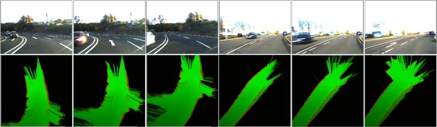
Contents

1   Introduction                                                                                                                  3

2   Deep Learning based Decision-Making Architectures for Self-Driving Cars                                                        3

3   Overview of Deep Learning Technologies                                                                                         4

    3.1   Deep Convolutional Neural Networks . . . . . . . . . . . . . . . . . . . . . . . . . . . . . . . . . . . . . .           4

    3.2   Recurrent Neural Networks . . . . . . . . . . . . . . . . . . . . . . . . . . . . . . . . . . . . . . . . . . . .        5

    3.3   Deep Reinforcement Learning . . . . . . . . . . . . . . . . . . . . . . . . . . . . . . . . . . . . . . . . . .          6

4   Deep Learning for Driving Scene Perception and Localization                                                                    8

    4.1   Sensing Hardware: Camera vs. LiDAR Debate . . . . . . . . . . . . . . . . . . . . . . . . . . . . . . . . .              8

    4.2   Driving Scene Understanding . . . . . . . . . . . . . . . . . . . . . . . . . . . . . . . . . . . . . . . . . . .        8

          4.2.1    Bounding-Box-Like Object Detectors . . . . . . . . . . . . . . . . . . . . . . . . . . . . . . . . . .          8

          4.2.2    Semantic and Instance Segmentation . . . . . . . . . . . . . . . . . . . . . . . . . . . . . . . . . . .        9

          4.2.3    Localization . . . . . . . . . . . . . . . . . . . . . . . . . . . . . . . . . . . . . . . . . . . . . . . .    9

    4.3   Perception using Occupancy Maps . . . . . . . . . . . . . . . . . . . . . . . . . . . . . . . . . . . . . . . .         10

5   Deep Learning for Path Planning and Behavior Arbitration                                                                      11

6   Motion Controllers for AI-based Self-Driving Cars                                                                             11

    6.1   Learning Controllers . . . . . . . . . . . . . . . . . . . . . . . . . . . . . . . . . . . . . . . . . . . . . . .      12

    6.2   End2End Learning Control . . . . . . . . . . . . . . . . . . . . . . . . . . . . . . . . . . . . . . . . . . . .        12

7   Safety of Deep Learning in Autonomous Driving                                                                                 14

8   Data Sources for Training Autonomous Driving Systems                                                                          16

9   Computational Hardware and Deployment                                                                                         19

10 Discussion and Conclusions                                                                                                     20

    10.1 Final Notes . . . . . . . . . . . . . . . . . . . . . . . . . . . . . . . . . . . . . . . . . . . . . . . . . . . .      21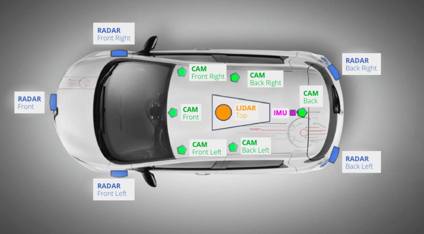
1    Introduction                                                2    Deep Learning based
                                                                      Decision-Making Architectures for
Over the course of the last decade, Deep Learning and Arti-
ficial Intelligence (AI) became the main technologies behind          Self-Driving Cars
many breakthroughs in computer vision [1], robotics [2] and      Self-driving cars are autonomous decision-making systems
Natural Language Processing (NLP) [3]. They also have a          that process streams of observations coming from different
major impact in the autonomous driving revolution seen to-       on-board sources, such as cameras, radars, LiDARs, ultra-
day both in academia and industry. Autonomous Vehicles           sonic sensors, GPS units and/or inertial sensors. These ob-
(AVs) and self-driving cars began to migrate from labora-        servations are used by the car’s computer to make driving
tory development and testing conditions to driving on pub-       decisions. The basic block diagrams of an AI powered au-
lic roads. Their deployment in our environmental landscape       tonomous car are shown in Fig. 1. The driving decisions are
offers a decrease in road accidents and traffic congestions,     computed either in a modular perception-planning-action
as well as an improvement of our mobility in overcrowded         pipeline (Fig. 1(a)), or in an End2End learning fashion
cities. The title of ”self-driving” may seem self-evident,       (Fig. 1(b)), where sensory information is directly mapped to
but there are actually five SAE Levels used to define au-        control outputs. The components of the modular pipeline
tonomous driving. The SAE J3016 standard [4] introduces          can be designed either based on AI and deep learning
a scale from 0 to 5 for grading vehicle automation. Lower        methodologies, or using classical non-learning approaches.
SAE Levels feature basic driver assistance, whilst higher        Various permutations of learning and non-learning based
SAE Levels move towards vehicles requiring no human in-          components are possible (e.g. a deep learning based object
teraction whatsoever. Cars in the level 5 category require       detector provides input to a classical A-star path planning al-
no human input and typically will not even feature steering      gorithm). A safety monitor is designed to assure the safety
wheels or foot pedals.                                           of each module.
   Although most driving scenarios can be relatively simply         The modular pipeline in Fig. 1(a) is hierarchically decom-
solved with classical perception, path planning and motion       posed into four components which can be designed using ei-
control methods, the remaining unsolved scenarios are cor-       ther deep learning and AI approaches, or classical methods.
ner cases in which traditional methods fail.                     These components are:
   One of the first autonomous cars was developed by Ernst
                                                                        • Perception and Localization,
Dickmanns [5] in the 1980s. This paved the way for new
research projects, such as PROMETHEUS, which aimed                      • High-Level Path Planning,
to develop a fully functional autonomous car. In 1994,
                                                                        • Behavior Arbitration, or low-level path planning,
the VaMP driverless car managed to drive 1, 600km, out
of which 95% were driven autonomously. Similarly, in                    • Motion Controllers.
1995, CMU NAVLAB demonstrated autonomous driving
                                                                    Based on these four high-level components, we have
on 6, 000km, with 98% driven autonomously. Another im-
                                                                 grouped together relevant deep learning papers describing
portant milestone in autonomous driving were the DARPA
                                                                 methods developed for autonomous driving systems. Addi-
Grand Challenges in 2004 and 2005, as well as the DARPA
                                                                 tional to the reviewed algorithms, we have also grouped rel-
Urban Challenge in 2007. The goal was for a driverless
                                                                 evant articles covering the safety, data sources and hardware
car to navigate an off-road course as fast as possible, with-
                                                                 aspects encountered when designing deep learning modules
out human intervention. In 2004, none of the 15 vehicles
                                                                 for self-driving cars.
completed the race. Stanley, the winner of the 2005 race,
                                                                    Given a route planned through the road network, the first
leveraged Machine Learning techniques for navigating the
                                                                 task of an autonomous car is to understand and localize it-
unstructured environment. This was a turning point in self-
                                                                 self in the surrounding environment. Based on this repre-
driving cars development, acknowledging Machine Learn-
                                                                 sentation, a continuous path is planned and the future ac-
ing and AI as central components of autonomous driving.
                                                                 tions of the car are determined by the behavior arbitration
The turning point is also notable in this survey paper, since
                                                                 system. Finally, a motion control system reactively corrects
the majority of the surveyed work is dated after 2005.
                                                                 errors generated in the execution of the planned motion. A
   In this survey, we review the different artificial intelli-
                                                                 review of classical non-AI design methodologies for these
gence and deep learning technologies used in autonomous
                                                                 four components can be found in [6].
driving, and provide a survey on state-of-the-art deep learn-
                                                                    Following, we will give an introduction of deep learning
ing and AI methods applied to self-driving cars. We also
                                                                 and AI technologies used in autonomous driving, as well as
dedicate complete sections on tackling safety aspects, the
                                                                 surveying different methodologies used to design the hierar-
challenge of training data sources and the required compu-
                                                                 chical decision making process described above. Addition-
tational hardware.
                                                                 ally, we provide an overview of End2End learning systems
                                                                 used to encode the hierarchical process into a single deep
                                                                 learning architecture which directly maps sensory observa-
                                                                 tions to control outputs.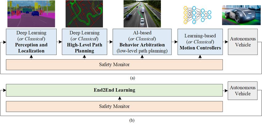
Figure 1: Deep Learning based self-driving car. The architecture can be implemented either as a sequential perception-
planing-action pipeline (a), or as an End2End system (b). In the sequential pipeline case, the components can be designed
either using AI and deep learning methodologies, or based on classical non-learning approaches. End2End learning systems
are mainly based on deep learning methods. A safety monitor is usually designed to ensure the safety of each module.

3     Overview of Deep Learning                                   automatically learn a representation of the feature space en-
                                                                  coded in the training set.
      Technologies                                                   CNNs can be loosely understood as very approximate
In this section, we describe the basis of deep learning tech-     analogies to different parts of the mammalian visual cor-
nologies used in autonomous vehicles and comment on               tex [12]. An image formed on the retina is sent to the visual
the capabilities of each paradigm. We focus on Convolu-           cortex through the thalamus. Each brain hemisphere has its
tional Neural Networks (CNN), Recurrent Neural Networks           own visual cortex. The visual information is received by the
(RNN) and Deep Reinforcement Learning (DRL), which are            visual cortex in a crossed manner: the left visual cortex re-
the most common deep learning methodologies applied to            ceives information from the right eye, while the right visual
autonomous driving.                                               cortex is fed with visual data from the left eye. The infor-
   Throughout the survey, we use the following notations to       mation is processed according to the dual flux theory [13],
describe time dependent sequences. The value of a variable        which states that the visual flow follows two main fluxes: a
is defined either for a single discrete time step t, written as   ventral flux, responsible for visual identification and object
superscript < t >, or as a discrete sequence defined in the       recognition, and a dorsal flux used for establishing spatial
< t,t + k > time interval, where k denotes the length of the      relations between objects. A CNN mimics the functioning
sequence. For example, the value of a state variable z is de-     of the ventral flux, in which different areas of the brain are
fined either at discrete time t, as z , or within a sequence   sensible to specific features in the visual field. The earlier
interval z . Vectors and matrices are indicated by bold    brain cells in the visual cortex are activated by sharp transi-
symbols.                                                          tions in the visual field of view, in the same way in which an
                                                                  edge detector highlights sharp transitions between the neigh-
3.1   Deep Convolutional Neural Networks                          boring pixels in an image. These edges are further used in
Convolutional Neural Networks (CNN) are mainly used for           the brain to approximate object parts and finally to estimate
processing spatial information, such as images, and can be        abstract representations of objects.
viewed as image features extractors and universal non-linear         An CNN is parametrized by its weights vector θ = [W, b],
function approximators [7], [8]. Before the rise of deep          where W is the set of weights governing the inter-neural
learning, computer vision systems used to be implemented          connections and b is the set of neuron bias values. The
based on handcrafted features, such as HAAR [9], Local Bi-        set of weights W is organized as image filters, with coef-
nary Patterns (LBP) [10], or Histograms of Oriented Gradi-        ficients learned during training. Convolutional layers within
ents (HoG) [11]. In comparison to these traditional hand-         a CNN exploit local spatial correlations of image pixels to
crafted features, convolutional neural networks are able to       learn translation-invariant convolution filters, which capture
discriminant image features.
Consider a multichannel signal representation Mk in layer
k, which is a channel-wise integration of signal representa-
tions Mk,c , where c ∈ N. A signal representation can be
generated in layer k + 1 as:
Mk+1,l = ϕ(Mk ∗ wk,l + bk,l ), (1)
where wk,l ∈ W is a convolutional filter with the same num- Figure 2: A folded (a) and unfolded (b) over time, many-
ber of channels as Mk , bk,l ∈ b represents the bias, l is a to-many Recurrent Neural Network. Over time t, both
channel index and ∗ denotes the convolution operation. ϕ(·) the input s and output z sequences share
is an activation function applied to each pixel in the input the same weights h . The architecture is also referred to
signal. Typically, the Rectified Linear Unit (ReLU) is the as a sequence-to-sequence model.
most commonly used activation function in computer vision
applications [1]. The final layer of a CNN is usually a fully- the learned weights in each unfolded copy of the network
connected layer which acts as an object discriminator on a are averaged, thus enabling the network to shared the same
high-level abstract representation of objects. weights over time.
In a supervised manner, the response R(·; θ ) of a The main challenge in using basic RNNs is the vanish-
CNN can be trained using a training database D = ing gradient encountered during training. The gradient sig-
[(x1 , y1 ), ..., (xm , ym )], where xi is a data sample, yi is the nal can end up being multiplied a large number of times,
corresponding label and m is the number of training exam- as many as the number of time steps. Hence, a traditional
ples. The optimal network parameters can be calculated us- RNN is not suitable for capturing long-term dependencies
ing Maximum Likelihood Estimation (MLE). For the clarity in sequence data. If a network is very deep, or processes
of explanation, we take as example the simple least-squares long sequences, the gradient of the network’s output would
error function, which can be used to drive the MLE process have a hard time in propagating back to affect the weights of
when training regression estimators: the earlier layers. Under gradient vanishing, the weights of
the network will not be effectively updated, ending up with
m very small weight values.
θ̂ = arg max L (θ ; D) = arg min ∑ (R(xi ; θ ) − yi )2 . (2) Long Short-Term Memory (LSTM) [17] networks are
θ θ i=1
non-linear function approximators for estimating temporal
dependencies in sequence data. As opposed to traditional
For classification purposes, the least-squares error is usually
recurrent neural networks, LSTMs solve the vanishing gra-
replaced by the cross-entropy, or the negative log-likelihood
dient problem by incorporating three gates, which control
loss functions. The optimization problem in Eq. 2 is typ-
the input, output and memory state.
ically solved with Stochastic Gradient Descent (SGD) and
Recurrent layers exploit temporal correlations of se-
the backpropagation algorithm for gradient estimation [14].
quence data to learn time dependent neural structures. Con-
In practice, different variants of SGD are used, such as
sider the memory state c and the output state h
Adam [15] or AdaGrad [16].
in an LSTM network, sampled at time step t − 1, as well as
the input data s at time t. The opening or closing of a
3.2 Recurrent Neural Networks gate is controlled by a sigmoid function σ (·) of the current
Among deep learning techniques, Recurrent Neural Net- input signal s and the output signal of the last time point
works (RNN) are especially good in processing temporal se- h , as follows:
quence data, such as text, or video streams. Different from
conventional neural networks, a RNN contains a time de- Γ
u = σ (Wu s + Uu h + bu ), (3)
pendent feedback loop in its memory cell. Given a time
dependent input sequence [s , ..., s ] and an output Γ
f = σ (W f s + U f h + b f ), (4)
sequence [z , ..., z ], a RNN can be ”unfolded”
τi + τo times to generate a loop-less network architecture
matching the input length, as illustrated in Fig. 2. t repre- Γo = σ (Wo s + Uo h + bo ), (5)
sents a temporal index, while τi and τo are the lengths of where Γu , Γ
f and Γ
o are gate functions of the input
the input and output sequences, respectively. Such neural gate, forget gate and output gate, respectively. Given current
networks are also encountered under the name of sequence- observation, the memory state c will be updated as:
to-sequence models. An unfolded network has τi + τo + 1
identical layers, that is, each layer shares the same learned
weights. Once unfolded, a RNN can be trained using the c = Γu ∗tanh(Wc s +Uc h +bc )+Γ f ∗c ,
backpropagation through time algorithm. When compared (6)
to a conventional neural network, the only difference is that The new network output h is computed as:• I is the set of observations, with I ∈ I defined as
h = Γ
o ∗ tanh(c ). (7) an observation of the environment at time t.
An LSTM network Q is parametrized by θ = [Wi , Ui , bi ], • S represents a finite set of states, s ∈ S being
where Wi represents the weights of the network’s gates the state of the agent at time t, commonly defined
and memory cell multiplied with the input state, Ui are the as the vehicle’s position, heading and velocity.
weights governing the activations and bi denotes the set of
neuron bias values. ∗ symbolizes element-wise multiplica- • A represents a finite set of actions allowing the
tion. agent to navigate through the environment defined
In a supervised learning setup, given by I , where a ∈ A is the action performed by
a set of training sequences D = the agent at time t.
[(s
, z1 ), ..., (s
, zq )], that is,
q independent pairs of observed sequences with assign- • T : S × A × S → [0, 1] is a stochastic transition func-
ments z , one can train the response of an LSTM tion, where Tss ,a describes the probability of
network Q(·; θ ) using Maximum Likelihood Estimation: arriving in state s , after performing action
a in state s .
θ̂ = arg max L (θ ; D) • R : S × A × S → R is a scalar reward function which
θ
m controls the estimation of a, where Rss ,a ∈ R.
= arg min ∑ li (Q(si ; θ ), z
), For a state transition s → s at time t, we
θ i=1 (8)
define a scalar reward function Rss ,a which
m τo
= arg min ∑ ∑ li (Q (si ; θ ), z ), quantifies how well did the agent perform in reach-
i
θ i=1 t=1 ing the next state.
where an input sequence of observations s = • γ is the discount factor controlling the importance
[s , ..., s , s ] is composed of τi consecutive data of future versus immediate rewards.
samples, l(·, ·) is the logistic regression loss function and t
represents a temporal index. Considering the proposed reward function and an arbi-
In recurrent neural networks terminology, the optimiza- trary state trajectory [s , s , ..., s ] in observation
tion procedure in Eq. 8 is typically used for training ”many- space, at any time tˆ ∈ [0, 1, ..., k], the associated cumulative
to-many” RNN architectures, such as the one in Fig. 2, future discounted reward is defined as:
where the input and output states are represented by tem- k
poral sequences of τi and τo data instances, respectively. R = ∑ γ r , (9)
This optimization problem is commonly solved using gradi- t=tˆ
ent based methods, like Stochastic Gradient Descent (SGD),
where the immediate reward at time t is given by r . In
together with the backpropagation through time algorithm
RL theory, the statement in Eq. 9 is known as a finite horizon
for calculating the network’s gradients.
learning episode of sequence length k [18].
The objective in RL is to find the desired trajectory policy
3.3 Deep Reinforcement Learning
that maximizes the associated cumulative future reward. We
In the following, we review the Deep Reinforcement Learn- define the optimal action-value function Q∗ (·, ·) which esti-
ing (DRL) concept as an autonomous driving task, using the mates the maximal future discounted reward when starting
Partially Observable Markov Decision Process (POMDP) in state s and performing actions [a , ..., a ]:
formalism.
In a POMDP, an agent, which in our case is the self-
driving car, senses the environment with observation I , Q∗ (s, a) = maxE [R |s = s, a = a, π], (10)
π
performs an action a in state s , interacts with its
environment through a received reward R , and tran- where π is an action policy, viewed as a probability density
sits to the next state s following a transition function function over a set of possible actions that can take place
Tss ,a . in a given state. The optimal action-value function Q∗ (·, ·)
In RL based autonomous driving, the task is to learn an maps a given state to the optimal action policy of the agent
to a
optimal driving policy for navigating from state sstart in any state:
destination state sdest , given an observation I at time
t and the system’s state s . I represents the observed ∀s ∈ S : π ∗ (s) = arg maxQ∗ (s, a). (11)
environment, while k is the number of time steps required a∈A
for reaching the destination state s
dest . The optimal action-value function Q∗ satisfies the Bell-
In reinforcement learning terminology, the above problem man optimality equation [19], which is a recursive formula-
can be modeled as a POMDP M := (I, S, A, T, R, γ), where: tion of Eq. 10:DeepMind in [22], where the combined algorithm, entitled
Rainbow, was able to outperform the independently compet-
∗ s0 s0 ∗ 0 0 ing methods. DeepMind [22] proposes six extensions to the
Q (s, a) = ∑ Ts,a Rs,a + γ · maxQ (s , a )
s a0 base DQN, each addressing a distinct concern:
(12)
s0 ∗ 0 0
= Ea0 Rs,a + γ · maxQ (s , a ) , • Double Q Learning addresses the overestimation
a0
bias and decouples the selection of an action and
where s0 represents a possible state visited after s = s its evaluation;
and a0 is the corresponding action policy. The model-based
• Prioritized replay samples more frequently from
policy iteration algorithm was introduced in [18], based on
the data in which there is information to learn;
the proof that the Bellman equation is a contraction map-
ping [20] when written as an operator ν: • Dueling Networks aim at enhancing value based
RL;
∀Q, lim ν (n) (Q) = Q∗ . (13)
n→∞
• Multi-step learning is used for training speed im-
However, the standard reinforcement learning method provement;
described above is not feasible in high dimensional state
spaces. In autonomous driving applications, the observa- • Distributional RL improves the target distribution
tion space is mainly composed of sensory information made in the Bellman equation;
up of images, radar, LiDAR, etc. Instead of the traditional
• Noisy Nets improve the ability of the network to ig-
approach, a non-linear parametrization of Q∗ can be en-
nore noisy inputs and allows state-conditional ex-
coded in the layers of a deep neural network. In litera-
ploration.
ture, such a non-linear approximator is called a Deep Q-
Network (DQN) [21] and is used for estimating the approx- All of the above complementary improvements have been
imate action-value function: tested on the Atari 2600 challenge. A good implementa-
tion of DQN regarding autonomous vehicles should start by
Q(s , a ; Θ) ≈ Q∗ (s , a ), (14) combining the stated DQN extensions with respect to a de-
where Θ represents the parameters of the Deep Q-Network. sired performance. Given the advancements in deep rein-
By taking into account the Bellman optimality equa- forcement learning, the direct application of the algorithm
tion 12, it is possible to train a deep Q-network in a rein- still needs a training pipeline in which one should simulate
forcement learning manner through the minimization of the and model the desired self-driving car’s behavior.
mean squared error. The optimal expected Q value can be The simulated environment state is not directly accessible
estimated within a training iteration i based on a set of ref- to the agent. Instead, sensor readings provide clues about the
erence parameters Θ̄i calculated in a previous iteration i0 : true state of the environment. In order to decode the true en-
vironment state, it is not sufficient to map a single snapshot
0
y = Rss,a + γ · maxQ(s0 , a0 ; Θ̄i ), (15) of sensors readings. The temporal information should also
a0 be included in the network’s input, since the environment’s
where Θ̄i := Θi0 . The new estimated network parameters state is modified over time. An example of DQN applied to
at training step i are evaluated using the following squared autonomous vehicles in a simulator can be found in [23].
error function: DQN has been developed to operate in discrete action
h i spaces. In the case of an autonomous car, the discrete ac-
∇JΘ̂i = min Es,y,r,s0 (y − Q(s, a; Θi ))2 , (16) tions would translate to discrete commands, such as turn
Θi left, turn right, accelerate, or break. The DQN approach de-
s0
where r = Rs,a . Based on 16, the maximum likelihood es- scribed above has been extended to continuous action spaces
timation function from Eq. 8 can be applied for calculating based on policy gradient estimation [24]. The method
the weights of the deep Q-network. The gradient is approx- in [24] describes a model-free actor-critic algorithm able to
imated with random samples and the backpropagation algo- learn different continuous control tasks directly from raw
rithm, which uses stochastic gradient descent for training: pixel inputs. A model-based solution for continuous Q-
learning is proposed in [25].
Although continuous control with DRL is possible, the
∇Θi = Es,a,r,s0 [(y − Q(s, a; Θi )) ∇Θi (Q(s, a; Θi ))] . (17) most common strategy for DRL in autonomous driving is
based on discrete control [26]. The main challenge here
The deep reinforcement learning community has made is the training, since the agent has to explore its environ-
several independent improvements to the original DQN al- ment, usually through learning from collisions. Such sys-
gorithm [21]. A study on how to combine these improve- tems, trained solely on simulated data, tend to learn a biased
ments on deep reinforcement learning has been provided by version of the driving environment. A solution here is to use
Imitation Learning methods, such as Inverse ReinforcementLearning (IRL) [27], to learn from human driving demon- The sensing approaches have advantages and disadvantages.
strations without needing to explore unsafe actions. LiDARs have high resolution and precise perception even in
the dark, but are vulnerable to bad weather conditions (e.g.
4 Deep Learning for Driving Scene heavy rain) [31] and involve moving parts. In contrast, cam-
eras are cost efficient, but lack depth perception and cannot
Perception and Localization work in the dark. Cameras are also sensitive to bad weather,
The self-driving technology enables a vehicle to operate au- if the weather conditions are obstructing the field of view.
tonomously by perceiving the environment and instrument- Researchers at Cornell University tried to replicate
ing a responsive answer. Following, we give an overview of LiDAR-like point clouds from visual depth estimation [32].
the top methods used in driving scene understanding, con- An estimated depth map is reprojected into 3D space, with
sidering camera based vs. LiDAR environment perception. respect to the left sensor’s coordinate of a stereo cam-
We survey object detection and recognition, semantic seg- era. The resulting point cloud is referred to as pseudo-
mentation and localization in autonomous driving, as well as LiDAR. The pseudo-LiDAR data can be further fed to 3D
scene understanding using occupancy maps. Surveys dedi- deep learning processing methods, such as PointNet [33]
cated to autonomous vision and environment perception can or AVOD [34]. The success of image based 3D estimation
be found in [28] and [29]. is of high importance to the large scale deployment of au-
tonomous cars, since the LiDAR is arguably one of the most
4.1 Sensing Hardware: Camera vs. LiDAR Debate expensive hardware component in a self-driving vehicle.
Deep learning methods are particularly well suited for de- Apart from these sensing technologies, radar and ultra-
tecting and recognizing objects in 2D images and 3D point sonic sensors are used to enhance perception capabilities.
clouds acquired from video cameras and LiDAR (Light De- For example, alongside three Lidar sensors, Waymo also
tection and Ranging) devices, respectively. makes use of five radars and eight cameras, while Tesla®
In the autonomous driving community, 3D perception is cars are equipped with eights cameras, 12 ultrasonic sensors
mainly based on LiDAR sensors, which provide a direct 3D and one forward-facing radar.
representation of the surrounding environment in the form
4.2 Driving Scene Understanding
of 3D point clouds. The performance of a LiDAR is mea-
sured in terms of field of view, range, resolution and ro- An autonomous car should be able to detect traffic partici-
tation/frame rate. 3D sensors, such as Velodyne® , usually pants and drivable areas, particularly in urban areas where a
have a 360◦ horizontal field of view. In order to operate at wide variety of object appearances and occlusions may ap-
high speeds, an autonomous vehicle requires a minimum of pear. Deep learning based perception, in particular Convolu-
200m range, allowing the vehicle to react to changes in road tional Neural Networks (CNNs), became the de-facto stan-
conditions in time. The 3D object detection precision is dic- dard in object detection and recognition, obtaining remark-
tated by the resolution of the sensor, with most advanced able results in competitions such as the ImageNet Large
LiDARs being able to provide a 3cm accuracy. Scale Visual Recognition Challenge [35].
Recent debate sparked around camera vs. LiDAR (Light Different neural networks architectures are used to detect
Detection and Ranging) sensing technologies. Tesla® and objects as 2D regions of interest [36] [37] [38] [39] [40] [41]
Waymo® , two of the companies leading the development or pixel-wise segmented areas in images [42] [43] [44] [45],
of self-driving technology [30], have different philosophies 3D bounding boxes in LiDAR point clouds [33] [46] [47], as
with respect to their main perception sensor, as well as re- well as 3D representations of objects in combined camera-
garding the targeted SAE level [4]. Waymo® is building LiDAR data [48] [49] [34]. Examples of scene perception
their vehicles directly as Level 5 systems, with currently results are illustrated in Fig. 3. Being richer in information,
more than 10 million miles driven autonomously2 . On the image data is more suited for the object recognition task.
other hand, Tesla® deploys its AutoPilot as an ADAS (Ad- However, the real-world 3D positions of the detected objects
vanced Driver Assistance System) component, which cus- have to be estimated, since depth information is lost in the
tomers can turn on or off at their convenience. The advan- projection of the imaged scene onto the imaging sensor.
tage of Tesla® resides in its large training database, con- 4.2.1 Bounding-Box-Like Object Detectors
sisting of more than 1 billion driven miles3 . The database
The most popular architectures for 2D object detection in
has been acquired by collecting data from customers-owned
images are single stage and double stage detectors. Pop-
cars.
ular single stage detectors are ”You Only Look Once”
The main sensing technologies differ in both companies.
(Yolo) [36] [50] [51], the Single Shot multibox Detector
Tesla® tries to leverage on its camera systems, whereas
(SSD) [52], CornerNet [37] and RefineNet [38]. Double
Waymo’s driving technology relies more on Lidar sensors4 .
stage detectors, such as RCNN [53], Faster-RCNN [54],
2 https://arstechnica.com/cars/2018/10/waymo- or R-FCN [41], split the object detection process into two
has-driven-10-million-miles-on-public-roads/ parts: region of interest candidates proposals and bounding
3 https://electrek.co/2018/11/28/tesla-
autopilot-1-billion-miles/ 4/19/17204044/tesla-waymo-self-driving-car-data-
4 https://www.theverge.com/transportation/2018/ simulationFigure 3: Examples of scene perception results. (a) 2D object detection in images. (b) 3D bounding box detector applied on
LiDAR data. (c) Semantic segmentation results on images.
boxes classification. In general, single stage detectors do ing drivable area, pedestrians, traffic participants, buildings,
not provide the same performances as double stage detec- etc. It is one of the high-level tasks that paves the way to-
tors, but are significantly faster. wards complete scene understanding, being used in appli-
If in-vehicle computation resources are scarce, one can cations such as autonomous driving, indoor navigation, or
use detectors such as SqueezeNet [40] or [55], which are virtual and augmented reality.
optimized to run on embedded hardware. These detectors Semantic segmentation networks like SegNet [42], IC-
usually have a smaller neural network architecture, making Net [43], ENet [57], AdapNet [58], or Mask R-CNN [45]
it possible to detect objects using a reduced number of oper- are mainly encoder-decoder architectures with a pixel-wise
ations, at the cost of detection accuracy. classification layer. These are based on building blocks from
A comparison between the object detectors described some common network topologies, such as AlexNet [1],
above is given in Figure 4, based on the Pascal VOC 2012 VGG-16 [59], GoogLeNet [60], or ResNet [61].
dataset and their measured mean Average Precision (mAP) As in the case of bounding-box detectors, efforts have
with an Intersection over Union (IoU) value equal to 50 and been made to improve the computation time of these sys-
75, respectively. tems on embedded targets. In [44] and [57], the authors
A number of publications showcased object detection proposed approaches to speed up data processing and infer-
on raw 3D sensory data, as well as for combined video ence on embedded devices for autonomous driving. Both
and LiDAR information. PointNet [33] and VoxelNet [46] architectures are light networks providing similar results as
are designed to detect objects solely from 3D data, pro- SegNet, with a reduced computation cost.
viding also the 3D positions of the objects. However, The robustness objective for semantic segmentation was
point clouds alone do not contain the rich visual informa- tackled for optimization in AdapNet [58]. The model is ca-
tion available in images. In order to overcome this, com- pable of robust segmentation in various environments by
bined camera-LiDAR architectures are used, such as Frus- adaptively learning features of expert networks based on
tum PointNet [48], Multi-View 3D networks (MV3D) [49], scene conditions.
or RoarNet [56]. A combined bounding-box object detector and semantic
The main disadvantage in using a LiDAR in the sensory segmentation result can be obtained using architectures such
suite of a self-driving car is primarily its cost5 . A solu- as Mask R-CNN [45]. The method extends the effective-
tion here would be to use neural network architectures such ness of Faster-RCNN to instance segmentation by adding a
as AVOD (Aggregate View Object Detection) [34], which branch for predicting an object mask in parallel with the ex-
leverage on LiDAR data only for training, while images are isting branch for bounding box recognition.
used during training and deployment. At deployment stage, Figure 5 shows tests results performed on four key seman-
AVOD is able to predict 3D bounding boxes of objects solely tic segmentation networks, based on the CityScapes dataset.
from image data. In such a system, a LiDAR sensor is nec- The per-class mean Intersection over Union (mIoU) refers to
essary only for training data acquisition, much like the cars multi-class segmentation, where each pixel is labeled as be-
used today to gather road data for navigation maps. longing to a specific object class, while per-category mIoU
refers to foreground (object) - background (non-object) seg-
4.2.2 Semantic and Instance Segmentation
mentation. The input samples have a size of 480px × 320px.
Driving scene understanding can also be achieved using se-
mantic segmentation, representing the categorical labeling 4.2.3 Localization
of each pixel in an image. In the autonomous driving con- Localization algorithms aim at calculating the pose (position
text, pixels can be marked with categorical labels represent- and orientation) of the autonomous vehicle as it navigates.
5 https://techcrunch.com/2019/03/06/waymo-to- Although this can be achieved with systems such as GPS, in
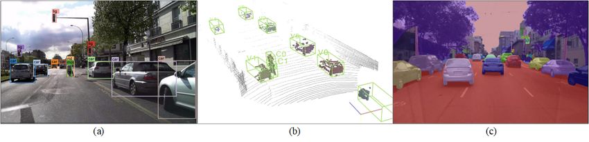
start-selling-standalone-lidar-sensors/ the followings we will focus on deep learning techniques forFigure 4: Object detection and recognition performance comparison. The evaluation has been performed on the Pas- cal VOC 2012 benchmarking database. The first four meth- ods on the right represent single stage detectors, while the remaining six are double stage detectors. Due to their in- Figure 5: Semantic segmentation performance compari- creased complexity, the runtime performance in Frames-per- son on the CityScapes dataset [74]. The input samples are Second (FPS) is lower for the case of double stage detectors. 480px × 320px images of driving scenes. visual based localization. with deep learning architectures able to automatically learn Visual Localization, also known as Visual Odometry the scene flow. In [73], an encoding deep network is trained (VO), is typically determined by matching keypoint land- on occupancy grids with the purpose of finding matching or marks in consecutive video frames. Given the current frame, non-matching locations between successive timesteps. these keypoints are used as input to a perspective-n-point Although much progress has been reported in the area mapping algorithm for computing the pose of the vehicle of deep learning based localization, VO techniques are with respect to the previous frame. Deep learning can be still dominated by classical keypoints matching algorithms, used to improve the accuracy of VO by directly influenc- combined with acceleration data provided by inertial sen- ing the precision of the keypoints detector. In [62], a deep sors. This is mainly due to the fact that keypoints detectors neural network has been trained for learning keypoints dis- are computational efficient and can be easily deployed on tractors in monocular VO. The so-called learned ephemeral- embedded devices. ity mask, acts a a rejection scheme for keypoints outliers which might decrease the vehicle localization’s accuracy. The structure of the environment can be mapped incremen- 4.3 Perception using Occupancy Maps tally with the computation of the camera pose. These meth- ods belong to the area of Simultaneous Localization and An occupancy map, also known as Occupancy Grid (OG), is Mapping (SLAM). For a survey on classical SLAM tech- a representation of the environment which divides the driv- niques, we refer the reader to [63]. ing space into a set of cells and calculates the occupancy Neural networks such as PoseNet [64], VLocNet++ [65], probability for each cell. Popular in robotics [72], [75], or the approaches introduced in [66], [67], [68], [69], or [70] the OG representation became a suitable solution for self- are using image data to estimate the 3D pose of a camera in driving vehicles. A couple of OG data samples are shown in an End2End fashion. Scene semantics can be derived to- Fig. 6. gether with the estimated pose [65]. Deep learning is used in the context of occupancy maps LiDAR intensity maps are also suited for learning a either for dynamic objects detection and tracking [76], prob- real-time, calibration-agnostic localization for autonomous abilistic estimation of the occupancy map surrounding the cars [71]. The method uses a deep neural network to build vehicle [77],[78], or for deriving the driving scene con- a learned representation of the driving scene from LiDAR text [79], [80]. In the latter case, the OG is constructed by sweeps and intensity maps. The localization of the vehicle accumulating data over time, while a deep neural net is used is obtained through convolutional matching. In [72], laser to label the environment into driving context classes, such scans and a deep neural network are used to learn descrip- as highway driving, parking area, or inner-city driving. tors for localization in urban and natural environments. Occupancy maps represent an in-vehicle virtual environ- In order to safely navigate the driving scene, an au- ment, integrating perceptual information in a form better tonomous car should be able to estimate the motion of the suited for path planning and motion control. Deep learning surrounding environment, also known as scene flow. Previ- plays an important role in the estimation of OG, since the ous LiDAR based scene flow estimation techniques mainly information used to populate the grid cells is inferred from relied on manually designed features. In recent articles, we processing image and LiDAR data using scene perception have noticed a tendency to replace these classical methods methods, as the ones described in this chapter of the survey.
Figure 6: Examples of Occupancy Grids (OG). The images show a snapshot of the driving environment together with its
respective occupancy grid [80].

5    Deep Learning for Path Planning                               NeuroTrajectory [85] is a perception-planning deep neural
                                                                   network that learns the desired state trajectory of the ego-
     and Behavior Arbitration                                      vehicle over a finite prediction horizon. Imitation learning
                                                                   can also be framed as an Inverse Reinforcement Learning
The ability of an autonomous car to find a route between           (IRL) problem, where the goal is to learn the reward func-
two points, that is, a start position and a desired location,      tion from a human driver [89], [27]. Such methods use real
represents path planning. According to the path planning           drivers behaviors to learn reward-functions and to generate
process, a self-driving car should consider all possible ob-       human-like driving trajectories.
stacles that are present in the surrounding environment and           DRL for path planning deals mainly with learning driv-
calculate a trajectory along a collision-free route. As stated     ing trajectories in a simulator [81], [90], [86] [87]. The real
in [81], autonomous driving is a multi-agent setting where         environmental model is abstracted and transformed into a
the host vehicle must apply sophisticated negotiation skills       virtual environment, based on a transfer model. In [81], it
with other road users when overtaking, giving way, merging,        is stated that the objective function cannot ensure functional
taking left and right turns, all while navigating unstructured     safety without causing a serious variance problem. The pro-
urban roadways. The literature findings point to a non triv-       posed solution for this issue is to construct a policy function
ial policy that should handle safety in driving. Considering a     composed of learnable and non-learnable parts. The learn-
reward function R(s̄) = −r for an accident event that should       able policy tries to maximize a reward function (which in-
be avoided and R(s̄) ∈ [−1, 1] for the rest of the trajectories,   cludes comfort, safety, overtake opportunity, etc.). At the
the goal is to learn to perform difficult maneuvers smoothly       same time, the non-learnable policy follows the hard con-
and safe.                                                          straints of functional safety, while maintaining an acceptable
   This emerging topic of optimal path planning for au-            level of comfort.
tonomous cars should operate at high computation speeds,              Both IL and DRL for path planning have advantages and
in order to obtain short reaction times, while satisfying spe-     disadvantages. IL has the advantage that it can be trained
cific optimization criteria. The survey in [82] provides a         with data collected from the real-world. Nevertheless, this
general overview of path planning in the automotive context.       data is scarce on corner cases (e.g. driving off-lanes, vehicle
It addresses the taxonomy aspects of path planning, namely         crashes, etc.), making the trained network’s response uncer-
the mission planner, behavior planner and motion planner.          tain when confronted with unseen data. On the other hand,
However, [82] does not include a review on deep learning           although DRL systems are able to explore different driving
technologies, although the state of the art literature has re-     situations within a simulated world, these models tend to
vealed an increased interest in using deep learning technolo-      have a biased behavior when ported to the real-world.
gies for path planning and behavior arbitration. Follow-
ing, we discuss two of the most representative deep learn-
ing paradigms for path planning, namely Imitation Learn-           6    Motion Controllers for AI-based
ing (IL) [83], [84], [85] and Deep Reinforcement Learning               Self-Driving Cars
(DRL) based planning [86] [87].
   The goal in Imitation Learning [83], [84], [85] is to learn     The motion controller is responsible for computing the lon-
the behavior of a human driver from recorded driving expe-         gitudinal and lateral steering commands of the vehicle.
riences [88]. The strategy implies a vehicle teaching pro-         Learning algorithms are used either as part of Learning Con-
cess from human demonstration. Thus, the authors em-               trollers, within the motion control module from Fig. 1(a), or
ploy CNNs to learn planning from imitation. For example,           as complete End2End Control Systems which directly map
sensory data to steering commands, as shown in Fig. 1(b). driving models [100], [101], driving dynamics for race cars
operating at their handling limits [102], [103], [104], as
6.1 Learning Controllers well as to improve path tracking accuracy [109], [91], [94].
Traditional controllers make use of an a priori model com- These methods use learning mechanisms to identify nonlin-
posed of fixed parameters. When robots or other au- ear dynamics that are used in the MPC’s trajectory cost func-
tonomous systems are used in complex environments, such tion optimization. This enables one to better predict distur-
as driving, traditional controllers cannot foresee every pos- bances and the behavior of the vehicle, leading to optimal
sible situation that the system has to cope with. Unlike con- comfort and safety constraints applied to the control inputs.
trollers with fixed parameters, learning controllers make use Training data is usually in the form of past vehicle states and
of training information to learn their models over time. With observations. For example, CNNs can be used to compute
every gathered batch of training data, the approximation of a dense occupancy grid map in a local robot-centric coor-
the true system model becomes more accurate, thus enabling dinate system. The grid map is further passed to the MPC’s
model flexibility, consistent uncertainty estimates and antic- cost function for optimizing the trajectory of the vehicle over
ipation of repeatable effects and disturbances that cannot be a finite prediction horizon.
modeled prior to deployment [91]. Consider the following A major advantage of learning controllers is that they op-
nonlinear, state-space system: timally combine traditional model-based control theory with
learning algorithms. This makes it possible to still use es-
z = ftrue (z , u ), (18) tablished methodologies for controller design and stability
analysis, together with a robust learning component applied
with observable state z ∈ Rnand control input u
∈ at system identification and prediction levels.
Rm , at discrete time t. The true system ftrue is not known
exactly and is approximated by the sum of an a-priori model 6.2 End2End Learning Control
and a learned dynamics model: In the context of autonomous driving, End2End Learning
Control is defined as a direct mapping from sensory data
z = f(z , u ) + h(z ) . (19) to control commands. The inputs are usually from a high-
a-priori model learned model
dimensional features space (e.g. images or point clouds).
In previous works, learning controllers have been intro- As illustrated in Fig 1(b), this is opposed to traditional pro-
duced based on simple function approximators, such as cessing pipelines, where at first objects are detected in the
Gaussian Process (GP) modeling [92], [93], [91], [94], or input image, after which a path is planned and finally the
Support Vector Regression [95]. computed control values are executed. A summary of some
Learning techniques are commonly used to learn of the most popular End2End learning systems is given in
a dynamics model which in turn improves an a Table 1.
priori system model in Iterative Learning Control End2End learning can also be formulated as a back-
(ILC) [96], [97], [98], [99] and Model Predictive Control propagation algorithm scaled up to complex models. The
(MPC) [100] [101], [91], [94], [102], [103], [104], [105], [106]. paradigm was first introduced in the 1990s, when the Au-
Iterative Learning Control (ILC) is a method for control- tonomous Land Vehicle in a Neural Network (ALVINN)
ling systems which work in a repetitive mode, such as path system was built [110]. ALVINN was designed to follow a
tracking in self-driving cars. It has been successfully ap- pre-defined road, steering according to the observed road’s
plied to navigation in off-road terrain [96], autonomous car curvature. The next milestone in End2End driving is con-
parking [97] and modeling of steering dynamics in an au- sidered to be in the mid 2000s, when DAVE (Darpa Au-
tonomous race car [98]. Multiple benefits are highlighted, tonomous VEhicle) managed to drive through an obstacle-
such as the usage of a simple and computationally light feed- filled road, after it has been trained on hours of human driv-
back controller, as well as a decreased controller design ef- ing acquired in similar, but not identical, driving scenar-
fort (achieved by predicting path disturbances and platform ios [111]. Over the last couple of years, the technological
dynamics). advances in computing hardware have facilitated the usage
Model Predictive Control (MPC) [107] is a control strat- of End2End learning models. The back-propagation algo-
egy that computes control actions by solving an optimiza- rithm for gradient estimation in deep networks is now ef-
tion problem. It received lots of attention in the last two ficiently implemented on parallel Graphic Processing Units
decades due to its ability to handle complex nonlinear sys- (GPUs). This kind of processing allows the training of large
tems with state and input constraints. The central idea and complex network architectures, which in turn require
behind MPC is to calculate control actions at each sam- huge amounts of training samples (see Section 8).
pling time by minimizing a cost function over a short End2End control papers mainly employ either deep neu-
time horizon, while considering observations, input-output ral networks trained offline on real-world and/or synthetic
constraints and the system’s dynamics given by a pro- data [119], [113], [114], [115], [120], [116], [117], [121], [118],
cess model. A general review of MPC techniques for au- or Deep Reinforcement Learning (DRL) systems trained
tonomous robots is given in [108]. and evaluated in simulation [23] [122], [26]. Methods for
Learning has been used in conjunction with MPC to learn porting simulation trained DRL models to real-world driv-Neural network Sensor
Name Problem Space Description
architecture input
ALVINN stands for Autonomous Land Vehicle In a Neural
3-layer Network). Training has been conducted using simulated
ALVINN Camera, laser
Road following back-prop. road images. Successful tests on the Carnegie Mellon
[110] range finder
network autonomous navigation test vehicle indicate that the
network can effectively follow real roads.
A vision-based obstacle avoidance system for off-road
DAVE 6-layer Raw camera mobile robots. The robot is a 50cm off-road truck, with two
DARPA challenge
[111] CNN images front color cameras. A remote computer processes the video
and controls the robot via radio.
Autonomous The system automatically learns internal representations of
NVIDIA PilotNet Raw camera
driving in real CNN the necessary processing steps such as detecting useful road
[112] images
traffic situations features with human steering angle as the training signal.
A generic vehicle motion model from large scale crowd-
Novel FCN-LSTM Ego-motion Large scale sourced video data is obtained, while developing an end-to
FCN-LSTM
[113] prediction video data -end trainable architecture (FCN-LSTM) for predicting a
distribution of future vehicle ego-motion data.
C-LSTM is end-to-end trainable, learning both visual and
Camera frames, dynamic temporal dependencies of driving. Additionally, the
Novel C-LSTM
Steering angle control C-LSTM steering wheel steering angle regression problem is considered classification
[114]
angle while imposing a spatial relationship between the output
layer neurons.
The sensor setup provides data for a 360-degree view of
CNN + Fully Surround-view the area surrounding the vehicle. A new driving dataset
Drive360 Steering angle and
Connected + cameras, CAN is collected, covering diverse scenarios. A novel driving
[115] velocity control
LSTM bus reader model is developed by integrating the surround-view
cameras with the route planner.
The trained neural net directly maps pixel data from a
DNN policy front-facing camera to steering commands and does not
Steering angle control CNN + FC Camera images
[116] require any other sensors. We compare the controller
performance with the steering behavior of a human driver.
DeepPicar is a small scale replica of a real self-driving car
DeepPicar called DAVE-2 by NVIDIA. It uses the same network
Steering angle control CNN Camera images
[117] architecture and can drive itself in real-time using a web
camera and a Raspberry Pi 3.
It incorporates Recurrent Neural Networks for information
TORCS
TORCS DRL Lane keeping and DQN + RNN integration, enabling the car to handle partially observable
simulator
[23] obstacle avoidance + CNN scenarios. It also reduces the computational complexity for
images
deployment on embedded hardware.
The image features are split into three categories (sky-related,
Steering angle control TORCS
TORCS E2E roadside-related, and roadrelated features). Two experimental
in a simulated CNN simulator
[118] frameworks are used to investigate the importance of each
env. (TORCS) images
single feature for training a CNN controller.
A CNN, refereed to as the learner, is trained with optimal
Steering angle and
Agile Autonomous Driving Raw camera trajectory examples provided at training time by an MPC controller.
velocity control CNN
[106] images The MPC acts as an expert, encoding the scene dynamics
for aggressive driving
into the layers of the neural network.
An Asynchronous ActorCritic (A3C) framework is used to
WRC6
WRC6 AD Driving in a CNN + LSTM learn the car control in a physically and graphically realistic
Racing
[26] racing game Encoder rally game, with the agents evolving simultaneously on
Game
different tracks.
Table 1: Summary of End2End learning methods.
ing have also been reported [123], as well as DRL systems on different road types. Prior to training, the data is enriched
trained directly on real-world image data [105], [106]. using augmentation, adding artificial shifts and rotations to
End2End methods have been popularized in the last cou- the original data.
ple of years by NVIDIA® , as part of the PilotNet architec- PilotNet has 250.000 parameters and approx. 27mil. con-
ture. The approach is to train a CNN which maps raw pixels nections. The evaluation is performed in two stages: first
from a single front-facing camera directly to steering com- in simulation and secondly in a test car. An autonomy per-
mands [119]. The training data is composed of images and formance metric represents the percentage of time when the
steering commands collected in driving scenarios performed neural network drives the car:
in a diverse set of lighting and weather conditions, as well asYou can also read