Austerity and the Rise of the Nazi Party - Cambridge ...
←
→
Page content transcription
If your browser does not render page correctly, please read the page content below
Austerity and the Rise of the Nazi Party
                          Gregori Galofré-Vilà, Christopher M. Meissner,
                                     Martin McKee, and David Stuckler

    We study the link between fiscal austerity and Nazi electoral success. Voting
    data from a thousand districts and a hundred cities for four elections between
    1930 and 1933 show that areas more affected by austerity (spending cuts and tax
    increases) had relatively higher vote shares for the Nazi Party. We also find that
    the localities with relatively high austerity experienced relatively high suffering
    (measured by mortality rates) and these areas’ electorates were more likely to vote
    for the Nazi Party. Our findings are robust to a range of specifications including
    an instrumental variable strategy and a border-pair policy discontinuity design.

I n 1928, the German Nazi Party earned just over 2 percent of the votes in
  the general federal elections. By mid-1932, it had received 38 percent of
votes in the national elections, becoming the largest political party in the
Reichstag. How did this shift to the extreme far-right happen so quickly?
Economic factors, such as high unemployment associated with the Great
Depression, sociocultural issues, and the excessively punitive Treaty of
Versailles, are well studied. They undoubtedly played an important role
in the rise of the Nazi Party. Still, the rapid growth of support for the Nazi
Party well into the Great Depression remains the subject of considerable

   The Journal of Economic History, Vol. 81, No. 1 (March 2021). © The Author(s), [2021].
Published by Cambridge University Press on behalf of the Economic History Association. This is
an Open Access article, distributed under the terms of the Creative Commons Attribution licence
(http://creativecommons.org/licenses/by/4.0/), which permits unrestricted re-use, distribution,
and reproduction in any medium, provided the original work is properly cited. doi: 10.1017/
S0022050720000601.
   Gregori Galofré-Vilà is Assistant Professor, Universidad Pública de Navarra, Department of
Economics, and Institute for Advanced Research in Business and Economics. E-mail: gregori.
galofre@unavarra.es. Christopher M. Meissner is Professor, Department of Economics,
University of California, Davis, and Research Associate at the NBER. E-mail: cmmeissner@
ucdavis.edu. Martin McKee is Professor, Department of Health Services Research and Policy,
London School of Hygiene & Tropical Medicine. E-mail: martin.mckee@lshtm.ac.uk. David
Stuckler is Professor, Department of Social and Political Sciences, University of Bocconi. E-mail:
david.stuckler@unibocconi.it.
   Earlier versions of this paper were presented at the Australian National University, Hitotsubashi
University, Humboldt University, the NBER, New York University, New York University–
Shanghai, Shanghai University of Finance and Economics, UC Berkeley, UC Davis, UC Irvine,
UCLA, the University of Groningen, the University of Michigan, and the 2018 World Economic
History Congress. We thank Maja Adena, Barbara Biasi, Fabio Braggion, Barry Eichengreen,
Ruben Enikolopov, Sanford Jacoby, Harold James, Peter Lindert, Dan Liu, Petra Moser, Maria
Petrova, Burkhard Schipper, Nico Voigtländer, Hans-Joachim Voth, and Noam Yuchtman for a
series of constructive suggestions. We also thank the editor, Dan Bogart, and four anonymous
referees for comments. DS is funded by a Wellcome Trust and European Research Council
Investigator Award (ERC HRES 313590).

                                                81
82        Galofré-Vilà, Meissner, McKee, and Stuckler

debate (Eichengreen 2018; Ferguson 1996; James 1986; Satayanth et al.
2017; Temin 1990; Voth 2020).
   In this paper, we investigate the association between the austerity
measures implemented by the German government between 1930 and
1932 and voters’ increased support for the Nazi Party. A growing liter-
ature studies the interactions between political preferences and fiscal
policy with evidence that austerity packages are correlated with rising
extremism (Alesina, Favero, and Giavazzi 2019; Bor 2017; Eichengreen
2015, 2018; Fetzer 2019; Ponticelli and Voth 2020). It stands to reason
that the austerity measures implemented in Germany in the early 1930s
played a role. However, we are aware of no direct quantitative assess-
ment of this issue for the Weimar Republic.
   During this period, Heinrich Brüning of the Center Party, and
Germany’s chancellor between March 1930 and May 1932, implemented
a set of measures via executive decree in order to balance the country’s
finances. These austerity measures included real cuts in spending and
transfers as well as higher tax rates. Brüning believed that the conse-
quent suffering would be highly visible, thereby eliciting international
sympathy for the Germans and helping put an end to the unpopular repa-
rations imposed at Versailles (Evans 2003).
   To test the hypothesis that austerity can explain increased Nazi vote
share, we use city and district-level election returns for the federal elec-
tions of 1930, 1932 (July and November), and 1933. We then link local
vote shares to different proxies for city, district, and state-level fiscal
policy changes while also controlling for other potential explanations
for the rise of the Nazis, such as unemployment, changes in wages,
and economic output. Our results are robust to inclusion of a number
of different controls and specifications including city-level time trends,
state by year fixed effects, and electoral district by year fixed effects.
   The observational data we use to study austerity and extremism have a
number of features that enable us to overcome obvious issues of reverse
causality and endogeneity. Brüning’s policies on spending and taxes
were not expected. Instead, they became an outcome of the unexpectedly
severe economic and financial crisis. They were decided at the Reich
level by Brüning and his cabinet with implicit support of the Reichstag.
Spending cuts and tax increases were uniformly applied across the nation
so that the policy decisions were exogenous to the preferences of specific
cities and districts. As noted by Balderston (1993, p. 225), “the progres-
sive ‘nationalization’ of taxing and spending decisions, justifies historians
in the responsibility they place on the Brüning cabinet and on Brüning
personally, for the fiscal balance during the slump.”
Austerity and the Rise of the Nazi Party                      83

   Limits on spending and on changes to taxes, policy variables often
formerly controlled by local authorities, were also imposed. Successive
pay cuts to national civil service salaries are an example. Although some
expenditure cuts were out of the hands of localities and mandated by the
national government, some budget categories were hit harder than others.
This fact means that nationally imposed budget cuts might have differential
impacts on localities depending on the predetermined patterns of spending
and reliance on the national government for transfers to fund different cate-
gories of spending. We use city-level variation in the preausterity reliance
on Reich transfers and national changes in transfers as a shift-share instru-
mental variable for subsequent spending declines. Since states, localities,
and the central government were unable to borrow on international capital
markets after 1930 (Schuker 1988), localities were forced by markets to
traverse the depression with highly disruptive fiscal shocks.
   As for taxes, a similar logic applies. The Reich maintained control
over a number of specific taxes, determining, for example, the statutory
marginal rates for income taxes and corporation turnover taxes. Changes
to the statutory marginal rates applied equally and evenly to all states and
localities, but lower brackets had higher percentage increases in income
tax rates (Newcomer 1936). We use variation at the local level in the
initial distribution of taxable income across tax brackets and national
changes in tax policy to instrument for the austerity-driven tax hikes. To
make identification valid, we need to avoid confounding our fiscal shock
with an unobservable economic shock correlated with income distribu-
tion. On the income distribution, Dell (2007) and Gómez-León and de
Jong (2019) show that Gini coefficients and top income shares were
fairly constant between 1928 and 1933.
   Higher Nazi vote share could be because of resentment arising from
distributional battles for slices of the fiscal pie in difficult times. There is
clearly a distributional component to these changes, the percentage rise
in tax rates being much higher for the lower income brackets. Wueller
(1933) also discusses that while tax revenue had traditionally been
retained where it was collected, intrastate redistribution was increasingly
becoming need based during the Depression.
   We also use a number of different econometric specifications to elimi-
nate further concerns about endogeneity. We employ both city/district
fixed effects models and long differences to focus on within-locality varia-
tion in Nazi support. We are also able to circumscribe the control group by
matching districts to neighboring districts just across state borders, as in
Dube, Lester, and Reich (2010). While relevant observables were spatially
smooth, fiscal policy across the state borders was sharply different because
84         Galofré-Vilà, Meissner, McKee, and Stuckler

state policies responded to statewide concerns. With this identification
strategy, we are also able to control for common economic shocks corre-
lated with the initial characteristics of localities by using period by district-
pair fixed effect interaction terms. Even after controlling for local economic
shocks between 1930 and 1932 in this way, austerity remains a statistically,
economically, and politically significant determinant of Nazi vote share.
   We also provide some novel quantitative estimates concerning the
channels by which austerity mattered. To do so, we study the relation-
ship between mortality rates and austerity. We find a plausible link,
since where public spending on health care dropped more, mortality was
higher. These places also saw a relatively large increase in Nazi support
at the polls. Finally, looking at archival documents of Nazi propaganda,
we document how Nazi leaders invoked austerity to attack Brüning and
the Weimar Republic and how Brüning’s tax rises were seen as ineffi-
cient and unfair by the German masses.
   Even though there has been a German debate on whether there was
an alternative to austerity (Borchardt 1980; Büttner 1989; Ritschl 1998;
Voth 1993) and speculation that austerity played a role in the rise of the
Nazi Party, to our knowledge, no previous research has directly tested the
quantitative impact and the channels by which fiscal austerity mattered.
Falter, Lindenberger, and Schumann (1986), Frey and Weck (1981), King
et al. (2008), and Stögbauer and Komlos (2004) studied the economic
shocks of the period, but they did not use fiscal data and the transmission
mechanisms emphasized are different from ours. Previous work focused
on a direct channel from lower disposable incomes and unemployment to
frustration at the polls. On global comparisons, one study evaluated the
impact of the Great Depression and austerity on voting patterns in 171
elections in 28 countries (Bromhead, Eichengreen, and O’Rourke 2013)
and another looked at the European level (Ponticelli and Voth 2020). Yet,
these have not considered the particular context of Weimar Germany.
   Regarding the connection between political competition and differential
effects of the crisis, the literature notes that the lowest status groups and the
unemployed turned to the Communists (Falter, Lindenberger, and Schumann
1986; King et al. 2008) but those just above in the economic hierarchy, who
had more to lose from the tax hikes and spending cuts, seemed to favor
the Nazis. Between 1930 and 1933 the Nazis gained votes from all walks
of life. Yet, Evans (2003), Falter, Lindenberger, and Schumann (1986),
King et al. (2008), and Voigtländer and Voth (2019) have documented how
the party was “underrepresented” among the working classes, in industrial
cities, and in Catholic regions. We control for these fixed factors and allow
for interactions between them and our measures of austerity.
Austerity and the Rise of the Nazi Party                    85

   Our baseline results show that Brüning’s austerity had a sizable effect.
Each one-standard-deviation increase in austerity was associated with
between one quarter to one half of one standard deviation of the depen-
dent variable. In localities where austerity was more severe, Nazi vote
share was significantly higher. Our novel use of within-locality variation
in the size of the fiscal shock sheds light on the local and national experi-
ence of democratic decline.
   The rest of the paper is organized as follows. In the next section, we
provide a detailed account of the main existing explanations for the rise
of the Nazis. The third and fourth sections, respectively, review how
austerity was implemented and present the historical context of the
different elections in Germany between 1930 and 1933. In the fifth and
sixth sections, we show our main results and robustness checks for the
city- and district-level outcomes using spending and tax data. The final
section concludes.

                     COMPETING EXPLANATIONS

   There are many competing explanations for the stark rise of the Nazi
Party in Weimar Germany. The conventional explanation is the impact
of the Great Depression. Those hit hardest by the economic downturn
held the incumbent parties responsible for their situation, punishing them
by voting for the Nazi Party. Economic activity peaked in Germany in
1928, driven by a sharp downturn in investment (Ritschl 2002; Temin
1971). Later, the cessation of capital inflows and a crisis in the German
banking sector culminated in a slowdown in the growth of credit, while
other international shocks prolonged the downturn. Yet, the unwilling-
ness of the Reichsbank to stop the deflation mattered but cannot neces-
sarily explain regional variation in Nazi support.
   A similar point could be made with respect to the increasing numbers
of unemployed workers, soaring from 1.4 million in 1928 to 5.6 million
in 1932. Unemployment also reached very high levels in other countries,
such as the United States, around that time, without being accompanied
by electoral radicalization (Eichengreen and Hatton 1988). Additionally,
the unemployed were more likely to vote for the Communist Party or
the Social Democrats (in Protestant precincts) rather than the Nazi Party
(Evans 2003; King et al. 2008), as the Communist Party was perceived as
the party that traditionally represented workers’ interests.
   A third explanation invokes resentment about high debt repayments
imposed on Germany in the Treaty of Versailles. These debts initially
totaled up to 260 percent of 1913 GDP (Ferguson 1997; Ritschl 2013).
86 Galofré-Vilà, Meissner, McKee, and Stuckler
Although France and Britain had war debt burdens similar to Germany,
the Versailles agreements treated Germany as a conquered enemy,
forcing it to pay a large share of the allies’ costs of the war. This placed
financial demands on Germany that were very difficult to meet and that
were dubbed as “cruel” by some (Keynes 1920; Temin and Vines 2014).
However, Germany’s war debts were never completely paid (Galofré-
Vilà et al. 2019). German war debts were postponed in the Hoover mora-
torium of 1931 or temporarily suspended in the Lausanne Conference a
year later.1
Fiscal austerity might simply have been a driver of economic collapse if
multipliers were large enough, but Ritschl (2013) reports that these were
small. If austerity mattered, it must have been something about the unique
way Germany experienced it. Even if austerity did not have a contrac-
tionary effect on aggregate demand, it still might have had distributional
consequences that, in turn, affected how people voted. Austerity not only
hurt the lower middle classes and elites, by increasing tax rates on profits
and income, but ostensibly also had a major impact on people’s welfare
by cutting key social spending lines after 1929. Brüning was commonly
known as the “Hunger Chancellor,” stressing how these budget cuts
threatened living conditions. There is, in fact, some qualitative consensus
on Brüning’s devastating legacy. Feinstein, Temin, and Toniolo (2008, p.
90) opine that “Brüning introduced a succession of austerity decrees. The
descent was cumulative and catastrophic.” Several authors also noted
that austerity could have contributed to political extremism. For instance,
Feldman (2005, p. 494) comments that “Brüning’s reliance on emergency
decrees had paved the way for a right-wing rule” and Eichengreen (2015,
p. 139) that “Brüning’s unrelenting austerity, by plunging the economy
deeper into recession, increased political polarization.”
Hitler also viewed austerity as a springboard to power. Twelve days
after Brüning enacted his fourth and last emergency decree, Hitler issued
a mass pamphlet titled The Great Illusion of the Last Emergency Decree.
He concluded the letter saying that “Although that was not the intention,
this emergency decree will help my party to victory, and therefore put
an end to the illusions of the present system.” There are also attacks on
Brüning’s cabinet on earlier fiscal plans. For instance, in October 1931,
Hitler wrote an Open Letter from Adolf Hitler to the Reich Chancellor in
1
Other explanations invoke the Weimar Republic’s electoral system, where each party was
allotted a number of seats in the Reichstag proportional to the votes received, which cleared the
path for small parties to enter the Reichstag (Jepsen 1953). Historians also stress the animosity
between the two major parties of the left and difficulties in building lasting coalitions. However,
Evans (2003) notes that proportional representation did not, in fact, encourage the rise of the
extreme right and alternative electoral systems might have given the Nazi Party even more seats.Austerity and the Rise of the Nazi Party 87
which he asked, “Where has the hereby-reduced number of unemployed
been left? Where are the successes of the ‘rescue of agriculture’? And
when, Mister Chancellor Brüning, did the then-promised reduction of
taxes finally begin?”
These pamphlets also made promises to relax the budget constraint
if the Nazis were elected. For instance, on May 1932, a pamphlet titled
Emergency Economic Program of the NSDAP offered “fundamental
improvements in agriculture in general, multiple years of taxation exemp-
tion for the settlers, cheap loans and the creation of markets by improving
transportation routes, and making them less expensive.” On the welfare
system, “National Socialism will do all it can to maintain the social insur-
ance system, which has been driven to collapse by the present System.” 2
Austerity and the German elections
In March 1930, Brüning was appointed as German Chancellor by
President von Hindenburg and fiscal reforms were quickly implemented,
with a first austerity plan in July 1930. Austerity was implemented
by emergency decree under Article 48 of the constitution, with the
Reichstag eventually consenting without formal debate. From its begin-
ning, austerity was highly unpopular, leading von Hindenburg to dissolve
the Reichstag and call new elections.3
In the elections of September 1930, the Social Democratic Party (SPD),
the political home of the worker movement, remained as the largest party
in the Reichstag (yet, moving from 29.8 percent of the total votes in May
1928 to 24.5 percent in 1930). The Center Party, which was Brüning’s
party, also started to lose popularity (moving from 12.1 to 11.8 percent),
and the Communist Party, the main party of protest for those workers
disenchanted by the Weimar regime, somewhat managed to collect new
votes (moving from 10.6 to 13.1 percent). The German National People’s
Party (DNVP), a bourgeois, xenophobic far-right party that shared many
of the Nazi’s extremist views, declined from 14.2 percent of total votes
to 7 percent. Above all these changes, support of the Nazi Party surged
from almost no support to more than 6 million voters (moving from less
than 3 percent to 18.3 percent).
2
There is also evidence that austerity formed part of Goebbels’ propaganda machine. For
instance, in a speech on 2 May 1931 at the Reichstag, Goebbels very prominently also alluded to
tax pressure on the middle class (Goebbels 1931). We thank Hans-Joachim Voth for calling this
speech to our attention.
3
Eichengreen (2018, p. 86) notes, “that the most dramatic cuts were imposed by decree,
circumventing normal legislative deliberation, did not foster popular admiration of the politicians
then in office or enhance the legitimacy of the constitutional system.”88 Galofré-Vilà, Meissner, McKee, and Stuckler
Although austerity was only implemented some months in advance,
the September 1930 election was a key turning point in German history
because it was seen as a withering verdict against austerity—a message
that went unheeded. As discussed by Temin (1990, p. 82), “…it is clear
that the vote of 1930 was a resounding rejection of Brüning’s policies
at an early stage.” Initially, only the Nazis (and, to some extent, the
Communists) campaigned against austerity, with the DNVP struggling to
find a coherent response on the austerity front. For instance, Fulda (2009,
p. 158) noted that for the first emergency decree, “the parliamentary
DNVP was split: while Hugenberg’s followers voted against it, the group
around Westarp decided to support it.” He also comments that when
“the tension between the pro-Brüning DNVP parliamentarians around
Westarp and Hugenberg’s supporters increased… Goebbels noted in his
diary that the DNVP was ‘finished’: ‘All grist to our mill.’”4 As for the
SPD, Brüning’s memoirs highlight that he often turned to members of the
SPD for support. Successive emergency decrees in June 1931, October
1931, and December 1931 raised nearly all of the main taxes controlled
by the Reich (income, wage, turnover, excise duties, tariffs), put limits on
spending, introduced exclusions from unemployment and relief benefits,
and mandated civil service pay cuts (over 50 percent of the state-level
spending bill according to Balderston (1993)).
By the end of May 1932, Brüning was removed from the Chancellorship
and was replaced by von Papen. The elections of July 1932 boosted Nazi
popularity even more, achieving 37.3 percent of the votes. Yet, the Nazis
lacked an overall majority at the Reichstag and von Papen continued
as Chancellor. In the second half of 1932, von Papen signaled the end
of austerity and started to introduce some stimulus packages, involving
employment programs, tax credits, and subsidies for new employment
and public works projects (Evans 2003; Feinstein, Temin, and Toniolo
2008). Despite the fact that any short-lived effect was modest in magni-
tude compared to the cumulative effect of Brüning’s austerity, the easing
of austerity, along with the ostensible cancellation of war debts at the
Lausanne conference and an improved economic environment,5 coin-
cided with a decline in Nazi vote share in the elections of November 1932
(collecting 33.1 percent of the votes). As O’Rourke (2010) comments,
“by this stage Brüning was gone, his successor adopted some modestly
4
By July 1930, the DNVP was split in two parties, with Westarp’s followers founding the
Konservative Volkspartei (supporting Brüning’s government) and the rest, commanded by
Hugenberg, radicalized and tried to approach the Nazi Party.
5
Between 1932 and 1933, real GDP grew by 6 percent. By comparison, real GDP fell by 8
percent between 1931 and 1932.Austerity and the Rise of the Nazi Party 89
stimulative policies, and there were signs of a partial recovery. Not coin-
cidentally, in November 1932 the Nazi share dipped to 33.1 percent; but
by then it was too late, and the Weimar Republic was doomed.”
Von Papen had virtually no support in the Reichstag, and in an ill-fated
attempt to increase his support, he called for new elections in November
of 1932. Yet, given mass discontent and social instabilities, later on,
Hindenburg appointed Schleicher of the DNVP as Chancellor.6 He lasted
for less than two months. Adolf Hitler was appointed chancellor on 30
January ahead of the decisive elections of March 1933, where the Nazi
Party became the largest party (with 44 percent of the votes) and built
a bare working majority with the DNVP that offered 8 percent of the
votes.7 These were the last elections of the Weimar Republic and were
tarnished by violence and intimidation and might not be regarded as free
and democratic.
Under Brüning’s mandate, there was a process of centralizing fiscal
policy and the national government began to limit the ability of states
to raise tax rates as well limited fiscal transfers to states and localities
(Balderston 1993).8 James (1986, p. 76) also commented that regional
governments were “left with odious taxes and falling revenues.” Although
austerity was determined at the Reich level, the extent to which it mattered
varied regionally. This variation depended on how lower levels of govern-
ment allocated their revenue to different types of expenditure and what
the sources of their tax revenues were. Around 40 percent of the spending
cuts were implemented by local authorities, mainly municipalities and
the so-called administrative divisions (Regierungsbezirke); 22 percent by
the different states; and around one-third by the Reich (Newcomer 1936).
Hence, the impact of Reich mandated cuts on the states varied according
to a number of predetermined fixed factors, including population and
land area, number of schools, highway mileage, and the distribution of
income (Newcomer 1936, p. 205).9
6
Schleicher also introduced some public works programs.
7
In the election of 1933, the DNVP presented in the elections as part of a coalition the
Kampffront Schwarz-Weiß-Rot, which was an electoral alliance of three parties: the DNVP, the
Stahlhelm, and Landbund.
8
There were two main bases for collection and redistributing revenue: origin and population.
While the origin base (returning revenue to the locality where it was collected) failed to take into
account the local need factor, redistribution by the population principle could be effective in terms
of “need.” Yet, the extent of redistribution depended on state political bargains and most of the
taxes in question were distributed on an origin basis (Wueller 1933, p. 38).
9
It is possible that greater unemployment also generated greater transfers via the unemployment
insurance scheme. Yet, by 1931, the period of eligibility for unemployment relief was drastically
restricted and nearly all people under 21 years were excluded from welfare benefits. These
measures were offset by the end of 1931 somewhat with greater relief payments and a partial
rollback of the exclusion (Balderston 1993).90 Galofré-Vilà, Meissner, McKee, and Stuckler
Political affinity to Brüning’s policies might have mattered, but in
essence, spending cuts were mandated at the central level. The room
to maneuver in the states was also highly constrained. States could no
longer borrow on international capital markets after 1930, and only a
small share of state spending was accounted for by local tax revenue over
which a state had control. While local politicians could potentially shift
spending between categories, the Reich increasingly dictated the way in
which states should spend money; put caps on spending categories; and,
in many instances, relied heavily on targeted Reich subsidies or transfers.
Thus, states were also constrained both by an inability to legislate tax rates
and by the traditional ways of redistributing tax revenue. Our bottom line
is that responding to the recession with discretionary spending was not
much of a possibility and both income tax10 and expenditure were largely
out of the hands of state governments and local authorities.11
Data
We collected data from official German sources (see our Online Data
Appendix for details and Galofré-Vilà et al. (2020)). Our analysis begins by
measuring the impact of austerity on electoral outcomes at the city level. Data
on electoral returns for the Reichstag elections are from the official publica-
tion Statistik des Deutschen Reiches (volumes Wahlem zum Reichstag), with
all the other data at the city level coming from the Statistisches Jahrbuch
Deutscher Städte, which report data for cities above 50,000 inhabitants (N
= 98). For each city, we collected city spending data for each fiscal year
from 1929/30 to 1932/33, which includes transfers from higher levels of
government and spending by budget category, in 1,000 RM. Such detailed
data at the city level allow us to look at the type of spending and the poten-
tial mechanisms by which spending changes can affect electoral outcomes.
The fiscal years ran from 1 April to 31 March, and when we say 1929, this
refers to the fiscal year 1929/30. We also collected data from the federal
transfers to cities (a variable called Überweisungen aus Reichsteuern) to
construct a Bartik-style instrument, as discussed subsequently.
To test competing explanations, we further used data on city-level
unemployment. Unemployment is defined as the number of people in the
labor force not working and registered in the local offices as unemployed.
We proxy city economic conditions by the construction of new residential
10
Income tax was a key tax in the Weimar revenue system (with 20 percent of total revenue).
11
Here, Newcomer (1936, p. 205) comments that “it is unfortunate that the equalizing factors
adopted have been vitiated in a number of instances by guarantees of pre-war income.” See also
Wueller (1933, p. 36).Austerity and the Rise of the Nazi Party 91
apartment buildings. We also collected mortality data from the bulletins
of the Reichs-Gesundheitsblatt. These bulletins report detailed mortality
data at the weekly level for cities with a population larger than 100,000
inhabitants (N = 51).
We also study district- (kreis-) level data (N = 1,024), where data
on taxes, but not spending, are available. Electoral and fiscal data on
taxes are from the official Statistik des Deutschen Reiches. For taxes, we
collected data on the number of taxpayers, total taxable income, and total
revenue for each state (in 1,000 RM) on two main federally administered
income taxes: the lohnsteuer, a withholding tax deducted at the source,
and the einkommenssteuer, an ex-post income declaration tax only paid
by middle and high rate payers. For the “wage tax” (lohnsteuer), data
are available in 1928/29 and 1932/33, and for the “income tax” (einkom-
menssteuer) for the years 1928/29, 1929/30, and 1932/33 (Dell 2007).
Despite missing data for some years, the available years allow us to
capture the main changes in taxation in the period of interest (September
1930–March 1933), and rather than having highly temporally disaggre-
gated data, we rely on benchmark years under the assumption that the
impact of austerity is cumulative. We also collected state-level data on
taxes (the lohnsteuer and einkommenssteuer) for the same years as in the
district sample.12
From the statistical abstracts Statistisches Jahrbuch für das Deutsche
Reich, we collected state-level data on spending, unemployment (number
of people in the labor force not working), an index of hourly wages,13 and
a proxy economic output (generation of electricity, in 1,000 kWh). For
the latter one, we use a proxy based on electricity generation, as these
two correlate closely, since the vast majority of goods and services are
produced using electricity. Other district-level data used in the Online
Data Appendix, such as the number of welfare recipients, are from Statistik
des Deutschen Reiches (volume Die Öffentliche Fürsorge im Deutschen
Reich). Table A1 reports the main summary statistics on key variables.
On the magnitude of austerity, as Figure 1 shows, between 1930 and
1932, state-level real expenditure was cut by 8 percent (nominal total
spending fell by about 25 percent) and Reich level real expenditure fell by
14 percent (30 percent nominal).14 These were not insignificant compo-
nents of aggregate demand since, together, state and Reich expenditure
totaled close to 30 percent of GDP in 1928/29.
12
For simplicity, when we say states, we also mean Prussian provinces.
13
We created a state-level index of nominal wages averaging the monthly data from the
hourly wages paid in four occupations (construction, wood, and skilled and unskilled workers in
metallurgy) in 38 large cities that are located within each of the states.
14
The spending data include transfers to other public authorities.92 Galofré-Vilà, Meissner, McKee, and Stuckler
Figure 1
DEVELOPMENT OF REAL PER CAPITA STATE SPENDING IN GERMANY,
1926/27–1932/33 (1926/27 = 100)
Notes: This figure shows the evolution of real per capita government spending between 1926/27
and 1932/33. Nominal state-level expenditure is as reported in James (1986) following fiscal
years and accounting for transfers to other public authorities. Data were originally collected from
Official Statistics (Statistiches Jahrbuch für das Deutsche Reich). Nominal expenditure has been
adjusted for inflation using the price index (1913/14 = 100) from Jürgen Sensch in HISTAT-
Datenkompilation online (Preisindizes für die Lebenshaltung in Deutschland 1924 bis 2001)
and for population using the data from Piketty and Zucman (Data Appendix for Capital is Back,
Table DE1).
Source: See the text.
Nazi support and city-level spending
With the launch of austerity in July 1930, the number of votes for
the Nazi Party soared from 6 to 14 million between the elections of
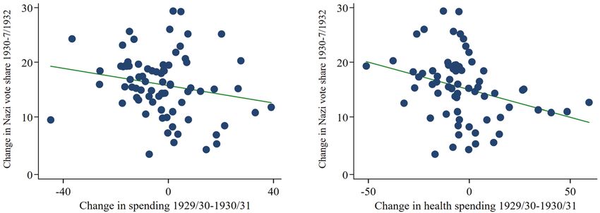
September 1930 and July 1932. Indeed, as Figure 2 suggests, there is a
close negative association between the increase in the Nazi vote share
between September 1930 and July 1932 and the change in city-level
spending between 1929/30 and 1930/31. We next explore these issues
more rigorously and implement some empirical strategies to limit biases
due to endogeneity.
Results
We begin our analysis reporting the results of statistical models where
the dependent variable is the level of the Nazi vote share across cities in
federal elections. We use city fixed effects throughout so that we relyAusterity and the Rise of the Nazi Party 93
Figure 2
CHANGES IN VOTE FOR THE NAZI PARTY AND CITY-LEVEL SPENDING,
1930–1932
Notes: Data on the y-axis are the difference in the vote share going to the Nazi Party between
the elections of September 1930 and July 1932. The x-axis shows the change in total city-level
government spending in percentage points (left figure) and the change in health and well-being
city-level government spending (right figure) in percentage points. The p-value in the right figure
is equal to 0.040 (r = –0.249) and in the left figure is equal to 0.009 (r = –0.320).
Source: See the text.
on within-city variation to identify the impact of austerity on Nazi vote
share. With these specifications, our models yield a difference-in-differ-
ences with an intensity of treatment interpretation based on
NAZIct = α + β1 ln (Expendituresct) + β2 ln (Unemploymentct) (1)
+ β3 ln (Outputct) + µc + δt + ect ,
where c is a city, t indexes elections, and NAZI denotes the vote share
of the Nazi Party as measured by the ratio of the number of votes to
the Nazi Party over the total number of (valid) votes cast. Expendituresct
comprises all categories of city expenditure, Unemploymentct is the
number of registered unemployed in a city, Outputct is our proxy for
economic output in a city, and ect is an error term. These control variables
are expressed in natural logarithms.15 We standardize data to have a mean
of zero and a standard deviation of one so coefficients across models are
directly comparable. We also include city fixed effects (µc) and fixed
effects for the calendar years of 1932 and 1933 (δt). We report standard
errors clustered at the administrative division level. There are 44 clusters,
and by clustering at the administrative division (above the city level), we
15
We use the values of city-level government spending for fiscal year 1929/30 for the election
of September 1930, values for 1931/32 for the elections of July and November 1932, and values
of 1932/33 for the election of 1933.94 Galofré-Vilà, Meissner, McKee, and Stuckler
Table 1
IMPACT OF CITY EXPENDITURES ON THE NAZI PARTY VOTE SHARE,
ALL NATIONAL ELECTIONS 1930–1933
(1) (2) (3) (4)
ln Expenditures –0.345** –0.415*** –0.351** –0.353**
(0.130) (0.133) (0.169) (0.155)
ln Unemployment 0.573 0.259 0.555***
(0.361) (0.183) (0.139)
ln Economic output 0.033 0.033 –0.255**
(0.044) (0.154) (0.122)
Number of observations 260 260 260 260
City-level fixed effect Yes Yes Yes Yes
Fixed effect 1932 Yes Yes No No
Fixed effect 1933 Yes Yes No No
State × period fixed effects No No Yes No
Admin. division × period fixed effects No No No Yes
Notes: Dependent variable is the percentage share (×100) of the valid votes cast going to the Nazi
Party in the different elections. Equation (1) is equivalent to the results we show in Column (2).
We use the controls of 1929 for the election of September 1930, 1931 for the elections of July and
November 1932, and 1932 for the election of March 1933. We estimate the linear models with
many levels of fixed effects, as in Correia (2017). We balance the sample for singleton groups and
use a balanced panel with robust standard errors (in parentheses) clustered on 44 administrative
divisions. We standardize all variables with a mean of zero and a standard deviation of one. ***p
< 0.01, **p < 0.05, *p < 0.1.
Source: See the text.
allow for arbitrary spatial correlations of the error term within the cluster.
Additionally, many of the variables were decided above the city level and
fixed effects already pick up potential spatial correlations.
In Table 1 (Column (2)), we show that a one-standard-deviation increase
in the natural logarithm of spending is associated with a decrease in Nazi
vote share (in standard deviation terms) of –0.42 (95 percent confidence
interval (CI): from –0.68 to –0.15). This specification, which pools data
for the four elections between 1930 and 1933, is robust to the inclusion
of administrative division or state by period fixed effects (Columns (3)
and (4)).16 These last specifications control for time-varying unobserv-
able shocks or arbitrary unobserved trends at the administrative division
or state level. Since shocks are likely to be highly spatially correlated,
these controls mop up the effect of spending changes after controlling for
local economic and political shocks.
16
Specifically, we interact state and administrative division level fixed effects with an indicator
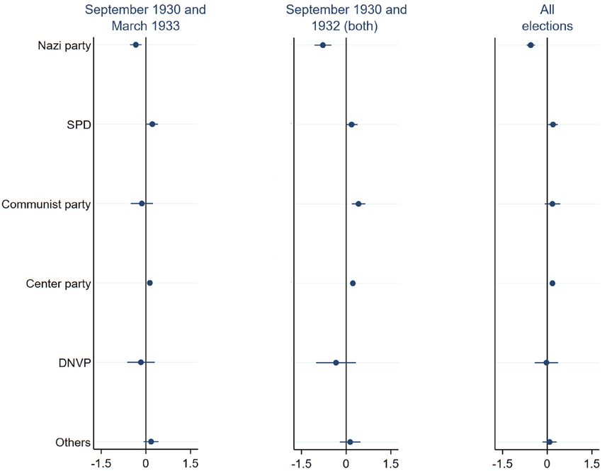
for each year 1932 and 1933.Austerity and the Rise of the Nazi Party 95 This table also displays the results for other competing explanations for the rise of the Nazi Party. Despite the fact that the coefficient on unemployment at the city-level displays a positive sign, it is only statisti- cally significant in Column (4). As Ferguson (1997, p. 267) notes, this is a likely outcome, as “it is a popular misconception that because high unemployment coincided with rising Nazi support, the unemployed must have voted for Hitler. Although some did, unemployed workers were more likely to turn to Communism than to Nazism.” When controlling for austerity and unemployment, in most cases, the economic output vari- able is also not statistically significant. Since we can differentiate party votes in the data, we next modify the outcome variable to be the vote share among other parties. This change allows us to see how austerity affected the rest of the German political spectrum. To also show that our results are not driven by a single elec- tion (or group of elections), we provide the results in three separate forest plots, pooling data for the elections of 1930 and 1933; elections of 1930 and 1932 (both elections); and the four elections between 1930 and 1933. Results for the Nazi Party in Figure 3 show that there is a negative and statistically significant association between spending and the Nazi Party vote share in the different elections between 1930 and 1933. Results for the other parties suggest that austerity mostly drew votes from the Center Party. This is not surprising as the Center Party was Brüning’s party and the party became very unpopular for consolidating the budget. For instance, Straumann (2019, p. 207) comments that “the harsh austerity measures of December 1931 … pushed the popularity of the Brüning cabinet down to a new low.” Results also display a positive sign for the SPD (although not always statistically significant) and the Communist Party (when avoiding the violent election of 1933). Results for the DNVP highlight its lack of a political position on the austerity front. Robustness Checks In Table A2, we also pool all elections and study the dynamics of the effects via interaction terms. Specifically, we interacted the spending data with a dummy for each election. Therefore, we estimated three coef- ficients, 7/1932, 11/1932, and 1/1933, and then one for austerity unin- teracted, which corresponds to the “omitted” category, which is 1930. In this way, we show that the austerity effect is stable across time, as the sample is kept stable and the reference point still remains 1930.
96            Galofré-Vilà, Meissner, McKee, and Stuckler

                                  Figure 3
        IMPACT OF CITY EXPENDITURES ON THE NAZI PARTY VOTE SHARE,
                        ELECTIONS 1930, 1932, AND 1933
Notes: Dependent variable is the percentage share (×100) of the valid votes cast going to the
main parties in the different elections. Models are estimated independently and adjusted for
unemployment and economic output. We use the controls of 1929 for the election of September
1930, 1931 for the elections of July and November 1932, and 1932 for the election of March 1933.
We use a balanced panel with robust standard errors clustered on 44 administrative divisions.
SPD stands for the Social Democratic Party and DNVP for the German National People’s
Party. In the election of 1933, the DNVP presented in the election as part of the Kampffront
Schwarz-Weiß-Rot, which was an electoral alliance of three parties: the DNVP, the Stahlhelm,
and Landbund. All models include city-level fixed effects, and the forest plot with the elections
1930 and 1932 (both) includes a fixed effect for 1931/32 and “all elections” fixed effects for 1932
and 1933. We standardized all variables with a mean of zero and a standard deviation of one.
Source: See the text.

We further test for the validity of our estimates in different ways.17 For
instance, in Table A3, we divide each of the right-hand-side variables by
population to show that our fixed effects models are very likely to proxy
for a stable population over the short horizon between 1930 and 1933.
   17
      We also used the data on the number of entries to the Nazi Party at the city level from
Satyanath, Voigtländer, and Voth (2017) and explored the impact of austerity on joining the Nazi
Party. Specifically, we looked at the log of the number of entries in the Nazi Party in the preceding
year and focused on the inflow of people into the party rather than on the stock of party members.
Using a specification equivalent to Equation (1) and pooling data from 1931 to 1933, the results
strengthen the case that nationalist and racist ideals became more salient when compounded by
austerity, driving people toward the Nazi ideology (Shirer 1960).
Austerity and the Rise of the Nazi Party 97
Table A4 further explores the interaction of the shock of the Depression
with social structure. We interacted year fixed effects with the share of
blue-collar workers in 1925 and the share of the population identifying
as Catholic or Protestant.18 The time interactions on religious identity
are significant, suggesting a role for such interaction. However, austerity
mattered in a similar way in Catholic and Protestant areas, though the
impact is higher in places with a Jewish community.19
Instrumental Variable and Endogeneity
One may worry that changes in spending were choice variables reflecting
the (unobservable) state of the underlying economy or the level of local
political competition. Politicians could alter spending levels in response
to these and their perceptions of these and other variables, making it prob-
lematic to infer the impact of exogenous changes in spending on votes
for an extreme party such as the Nazis. To deal with the potential endo-
geneity of expenditures, we employ a shift share instrumental variable in
the spirit of Aizer (2010), which relies on variation at the national level
in “across-the-board” cuts imposed by Brüning. Consider the following
stylized equation for total government spending G in city c in fiscal year t:
Gct = GFct + GLct.
(2)
Spending in city c is composed of two components. One is federal trans-
fers or the federally mandated level of spending GFct. This variable could
also be construed as local spending based on local claims to federal revenue
streams, where the subscript F denotes federal transfers or mandates to
city c. The other component, GLct, is based on local decision-making and
local revenues. Assuming that this spending is constant, the change in total
spending between period t and period t – 1 given an (α – 1) percent change
in federal spending applied to all localities (0 ≤ α ≤ 1) is given by
G
% ∆Gct = Fct−1 × (α − 1). (3)
Gct−1
The absolute value of the percentage change in spending is directly
related to the share of federal spending in total city spending. That is,
18
Using Equation (1), we also split the sample for Prussian and non-Prussian cities and found
that in both cases results are negative and statistically significant, with point estimates being
larger in Prussian cities.
19
In Table A5, we also show that results hold when we control for the severity of the depression
using data on the number of welfare recipients. While this variable might be colinear with
spending, not controlling for spending but for the number of recipients suggests that expectations
might also have mattered. People could also respond to perceived austerity rather than actual
exposure to austerity.98 Galofré-Vilà, Meissner, McKee, and Stuckler
the larger the share of GFct–1 in Gct–1, the larger the percentage fall in
total spending, (%∆Gct ), for a (α –1)% change in GFct–1. Our instrument,
therefore, is the initial share of federal transfers in total city spending in
1929 interacted with year indicators represented by δt , which themselves
proxy for the across-the-board nationally imposed spending cuts. This
two-stage least squares (2SLS) approach is reminiscent of Nakamura and
Steinsson (2014) or Chodorow-Reich et al. (2012).
⎡⎛ G ⎞ ⎤
To satisfy exogeneity, we assume that E ⎢⎜ Fc1929 ⋅ δ t ⎟ ect ⎥ = 0 . In a
⎢⎣⎝ Gc1929 ⎠ ⎥⎦
broader survey on shift-share instruments, Goldsmith-Pinkham, Sorkin,
⎛ GFc1929 ⎞
and Swift (2020) argue that if initial shares are exogenous, the
⎜⎝ G ⎟⎠
c1929
Bartik-style or shift-share instrument boils down to using initial shares
(interacted with time dummies) as excluded instruments. With two
sectors, they also show it is only necessary to use one sector share and
this is equivalent to a Bartik approach. To satisfy the exclusion restric-
tion, one would have to believe that reliance on the central government
in 1929 was not related to the unobservables driving the change in Nazi
vote share. As suggested by Goldsmith-Pinkham, Sorkin, and Swift
(2020), we tested this by regressing the initial share on observables such
as the share of Protestants and Catholics, levels of unemployment, or the
construction of new buildings. In none of the cases were these variables
statistically significant. For relevance, the log deviation in spending from
the within-city mean must be correlated with the initial dependency on
the Reich transfers. This would evidently be true unless local spending
changes completely offset (orthogonal) Reich spending changes. This is
not possible since localities could not fund spending by borrowing due to
financial market dislocation and due to the fact that total tax revenue was
falling as a result of the decline in aggregate activity.
As Table 2 shows, using ordinary least squares (OLS), the impact
in terms of standard deviations in vote share for the Nazi Party asso-
ciated with a one-standard-deviation increase in the percentage change
in spending is –0.78 (95 percent CI: from –1.21 to –0.34) in the elec-
tions of 1930 and 1932 (both) and –0.55 (95 percent CI: from –0.77 to
–0.34) when considering all elections.20 Results using 2SLS are just 15
percent larger (in absolute magnitude) than the OLS results in Column
20
We also checked for linearity, categorizing the spending data into bins and including the
dummy variables for the bins in the model. We also explored this with bins of different sizes in
the spending data. The assumption of linearity is largely suitable.Austerity and the Rise of the Nazi Party 99
Table 2
IMPACT OF CITY EXPENDITURES ON THE NAZI PARTY VOTE SHARE USING
A BARTIK INSTRUMENT, NATIONAL ELECTIONS 1930, 1932, AND 1933
Elections 1930 and 1932 (Both) All Elections
OLS 2SLS OLS 2SLS
(1) (2) (3) (4)
ln Expenditures –0.781*** –0.896** –0.553*** –0.683**
(0.215) (0.444) (0.108) (0.337)
ln Unemployment 1.008** 1.012*** 0.654** 0.682***
(0.412) (0.379) (0.295) (0.233)
ln Economic output –0.014 –0.009 0.020 0.019
(0.118) (0.093) (0.044) (0.053)
F-test excluded instrument 14.16 20.69
Rubin–Anderson test (p-value) 0.017 0.042
Number of cities 231 231 308 308
City-level fixed effect Yes Yes Yes Yes
Fixed effect 1931/32 Yes Yes Yes Yes
Fixed effect 1932/33 No No Yes Yes
Notes: Dependent variable is the percentage share (×100) of the valid votes cast going to the main
parties in the different elections. We use the controls of 1929 for the election of September 1930,
1931 for the elections of July and November 1932, and 1932 for the election of March 1933.
The first-stage coefficient on the initial average income tax rate is negative and highly significant
(–0.103; p-value = 0.000; 95 percent CI: –0.129 to –0.077). We use a balanced panel with standard
errors clustered on 44 administrative divisions. For details on the instrument, refer to the text. All
models include time and city-level fixed effects. We standardize all variables with a mean of zero
and a standard deviation of one. ***p < 0.01, **p < 0.05, *p < 0.1.
Source: See the text.
(4), showing that OLS results may not be highly biased. In Table A6, we
also show the Bartik results using models in differences.
Mechanisms
In Figure 4, we modify Equation (1) and, instead of all city-level
expenditure, we study the impact of changes in different types of expen-
diture. Interestingly, most of the effect of austerity is driven by spending
changes in health and well-being (–1.03: 95 percent CI: from –1.53 to
–0.52) and housing (–0.21: 95 percent CI: from –0.39 to –0.03). These
were among the budgets most affected by austerity.21 The size of the effect
for spending changes in health and well-being is 32 percent higher than
21
As noted by Straumann (2019, p. 70) on the Second Emergency Decree, “the plan proposed
a series of spending cuts, notably of health insurance compensations and of revenues apportioned
to states and municipalities.”100 Galofré-Vilà, Meissner, McKee, and Stuckler
Figure 4
IMPACT OF CITY EXPENDITURES BY BUDGET CATEGORY ON THE NAZI PARTY
VOTE SHARE, ELECTIONS 1930, 1932, AND 1933
Notes: Dependent variable is the percentage share (×100) of the valid votes cast going to the
Nazi Party in the different elections. Models are estimated independently and adjusted for
unemployment and economic output. We use the controls of 1929 for the election of September
1930, 1931 for the elections of July and November 1932, and 1932 for the elections of March 1933.
We use a balanced panel with robust standard errors clustered on 44 administrative divisions. All
models include city-level fixed effects, and the forest plot with the elections 1930 and 1932 (both)
includes a fixed effect for 1931/32 and “all elections” fixed effects for 1931/32 and 1932/33. We
standardized all variables with a mean of zero and a standard deviation of one.
Source: See the text.
the overall effects of the spending changes presented in the previous table,
showing that social spending changes plausibly exacerbated the suffering
of the German masses. There is also a positive effect of expenditure in
construction and the Nazi vote share between the elections of September
1930 and 1933. As we have already seen, by the end of 1932, von Papen
and Schleicher introduced some tax discounts as well as construction and
work programs, which, along with Hitler’s promise to construct an auto-
bahn, were symbols of a new era of economic competence and the end
of austerity (Voigtländer and Voth 2019). However, the effect disappears
when we introduce data for the austerity years and the elections of 1932.
The literature also stresses that Brüning’s fiscal plans were part of a polit-
ical strategy to elicit international sympathy for German suffering, puttingAusterity and the Rise of the Nazi Party 101
an end to WWI reparations.22 Coinciding with the fiscal retrenchment,
mortality rates, which had been declining, started to rise rapidly after 1932.
One mechanism for the rise of populist parties is that they gain the most
votes where health fares worst. This link was outlined by some commenta-
tors at the time. For instance, by the fall of October 1930, Hjalmar Schacht
(former head of the Reichsbank) gave an interview to the American press
saying that, “If the German people are going to starve, there are going to be
many more Hitlers” (The New York Times, 3 October 1930).
Next, we report suggestive evidence that the effect of spending cuts
was through the channel of higher mortality. In Table 3, we use Equation
(1) and also add a control for mortality. Since we use city fixed effects,
mortality here can be interpreted as excess mortality, that is, within-city
changes or deviations of mortality from its within-sample mean. Instead of
overall spending, we use only spending in health and well-being. Column
(1) shows that after controlling for unemployment and economic output
and other fixed effects, increases in spending are negatively and statisti-
cally related to Nazi Party vote. Similarly, Column (2) shows that without
controlling for spending, higher mortality is associated with higher Nazi
vote share. However, once we add the mortality control (Column (3)),
expenditure is no longer statistically significant and the size of the coef-
ficient declines by 34 percent. If we remove the deaths from cancers and
a category for ill-defined causes, the coefficient for mortality remains
statistically significant at the 1 percent level of confidence (Column (5)),
but the coefficient on spending declines by more than half and is not
statistically significant. Although results are weaker for infant mortality,
possibly because births to the poorest families fall disproportionately
during a recession (Dehejia and Lleras-Muney 2004), they display a low
p-value (Column (7)). This result further illustrates that the impact of
austerity was potentially channeled through suffering (as measured by
changes in mortality). It is also interesting that the coefficients on unem-
ployment and economic output, once we control for austerity, are similar
before and after we include the mortality control.
Nazi support and district-level taxes
Results
We next move to district-level data. Since spending data at the district
level are unavailable from national sources, we rely on within-district
22
This strategy was never a clear political winner and soon lacked an economic rationale. By
June 1931, the Hoover Moratorium had suspended Germany’s WWI debts for one year. A year
later, in July 1932, reparations were permanently postponed at the Lausanne Conference.Table 3
IMPACT OF CITY EXPENDITURES IN HEALTH AND WELL-BEING AND MORTALITY ON THE NAZI PARTY VOTE SHARE,
102
ALL NATIONAL ELECTIONS 1930–1933
(1) (2) (3) (4) (5) (6) (7)
ln Expenditures: health and well-being –0.237* –0.156 –0.101 –0.197
(0.128) (0.129) (0.110) (0.120)
ln Mortality 0.173** 0.152* 0.232*** 0.218*** 0.089* 0.073
(0.071) (0.085) (0.062) (0.071) (0.052) (0.053)
ln Unemployment 0.785** 0.690** 0.726** 0.663** 0.688** 0.739** 0.777**
(0.331) (0.290) (0.288) (0.273) (0.269) (0.305) (0.311)
ln Economic output –0.029 –0.074 –0.069 –0.073 –0.071 –0.028 –0.030
(0.070) (0.075) (0.076) (0.072) (0.073) (0.073) (0.072)
Number of observations 150 150 150 150 150 150 150
City-level fixed effect Yes Yes Yes Yes Yes Yes Yes
Fixed effect for 1932 Yes Yes Yes Yes Yes Yes Yes
Fixed effect for 1933 Yes Yes Yes Yes Yes Yes Yes
Baseline Yes No No No No No No
All deaths No Yes Yes No No No No
No deaths from cancer No No No Yes Yes No No
Infant mortality No No No No No Yes Yes
Notes: Dependent variable is the percentage share (×100) of the valid votes cast going to the Nazi Party in the different elections. We use the controls of 1929 for the
election of September 1930, 1931 for the elections of July and November 1932, and 1932 for the election of March 1933. Column (1) is the baseline specification
without controlling for mortality. In Columns (2) and (3), the Crude Death rate is the number of deaths within a city divided by the city-level population (×1,000).
In Columns (4) and (5), from the Crude Death rate, we removed deaths from cancer and unspecified causes of death. In Columns (6) and (7) is the Infant Mortality
Galofré-Vilà, Meissner, McKee, and Stuckler
rate measured as the number of deaths within a city below the age of one divided by the number of live births (×1,000). We use a balanced panel with robust standard
errors (in parentheses) clustered on 30 administrative divisions. All models include city level fixed effects. We also add fixed effects for 1931/32 and 1932/33. We
standardize all variables with a mean of zero and a standard deviation of one. ***p < 0.01, **p < 0.05, *p < 0.1.
Source: See the text.You can also read