Auto-context and Its Application to High-level Vision Tasks
←
→
Page content transcription
If your browser does not render page correctly, please read the page content below
Auto-context and Its Application to High-level Vision Tasks

                                                Zhuowen Tu
                          Lab of Neuro Imaging, University of California, Los Angeles
                                                    ztu@loni.ucla.edu

                         Abstract                                    sented by the joint statistics of the multi-variate in the pos-
                                                                     terior probability, which is decomposed into likelihood and
    The notion of using context information for solving high-        prior. In vision, likelihood and prior are often referred to as
level vision problems has been increasingly realized in the          appearance and shape respectively. However, there are still
field. However, how to learn an effective and efficient con-         many technological hurdles to overcome and the difficulties
text model, together with the image appearance, remains              can be summarized into two aspects: modeling and comput-
mostly unknown. The current literature using Markov Ran-             ing. (1) Difficulty in modeling complex appearances: Ob-
dom Fields (MRFs) and Conditional Random Fields (CRFs)               jects in natural images observe complex patterns. There are
often involves specific algorithm design, in which the mod-          many factors contributing to the complexity such as texture
eling and computing stages are studied in isolation. In this         (homogeneous or inhomogeneous), lighting conditions, and
paper, we propose an auto-context algorithm. Given a set             occlusion. (2) Difficulty in learning complicated shapes.
of training images and their corresponding label maps, we            (3) Difficulty in computing for the optimal solution: The
first learn a classifier on local image patches. The discrimi-       optimal solution is often considered as the one which maxi-
native probability (or classification confidence) maps by the        mizes a posterior (MAP), or equivalently, minimizes an en-
learned classifier are then used as context information, in          ergy. Searching for the optimal solution for the combination
addition to the original image patches, to train a new clas-         of the appearance and shape models is an non-trivial task.
sifier. The algorithm then iterates to approach the ground               From the energy minimization point of view, models like
truth. Auto-context learns an integrated low-level and con-          Markov Random Fields (MRFs) [6], conditional Markov
text model, and is very general and easy to implement. Un-           Random Fields (CRFs) [9], and computing algorithms such
der nearly the identical parameter setting in the training,          as Belief Propagation (BP) [15, 30], have been widely used
we apply the algorithm on three challenging vision applica-          in vision [21]. However, these models and algorithms share
tions: object segmentation, human body configuration, and            somewhat similar disadvantages: (1) the choice of functions
scene region labeling. It typically takes about 30 ∼ 70 sec-         used are quite limited so far; (2) they usually rely on a fixed
onds to run the algorithm in testing. Moreover, the scope            topology with very limited neighborhood relation; (3) they
of the proposed algorithm goes beyond high-level vision. It          are slow in solving many real vision problems, whereas bio-
has the potential to be used for a wide variety of problems          logical vision systems can identify and understand complex
of multi-variate labeling.                                           objects/scenes very rapidly; (4) they are only guaranteed to
                                                                     obtain the optimal solution for a limited function families.
                                                                     Hidden Markov models (HMM) [12] studies the depen-
1. Introduction
                                                                     dencies of the neighboring states, which is in a way similar
    It has been noted that context and high-level information
                                                                     to the MRFs. HMM is also limited to short range context
plays a vital role in object and scene understanding [2, 22].
                                                                     information and usually is time consuming in learning the
Yet, a principled way of learning an effective and efficient
                                                                     parameters and computing for the solutions.
context model, together with the image appearance, is not
available. Context comes into a variety of forms and it can              From the point of view of using context information,
be referred to as Gestalt laws in middle level knowledge,            there have been a lot of recent work proposed in object
intra-object configuration, and inter-object relationship. For       recognition and scene understanding [8, 19, 16, 22, 18, 28,
example, a clear horse face may suggest the location of its          7, 20]. A pioneering work was proposed by Belongie et
tail and legs, which are often occluded or not easy to iden-         al. [2] which uses shape context in shape matching.
tify. The strong appearance of a car might well suggest the            In this paper, we make an effort to address some of the
existence of a road, and vice versa [8].                             questions mentioned above by proposing an auto-context
    From the Bayesian statistics point view, context is repre-       model. The algorithm targets the posterior distribution di-

                                                                 1
rectly in a supervised approach. Like in the BP algo-             boosting algorithm. The auto-context is a general algorithm
rithm [30], the goal is to learn/compute the marginals of         and the classifier of choice is not limited to boosting al-
the posterior, which we also call classification maps for the     gorithms. It directly targets the posterior through iterative
rest of this paper. Each training image comes with a label        steps, resulting in a simpler and more efficient algorithm
map in which every pixel is assigned with a label of interest.    than BRFs and SpatialBoost. Under nearly the same set of
A classifier is first trained to classify each pixel. There are   parameters in training, we demonstrate several applications
two types of features for the classifier to choose from: (1)      using the auto-context, which are not available in [22, 1].
image features computed on the local image patches cen-           A feed forward way of including context with appearance
tered at the current pixel (we use image patches of fixed         was proposed in [28] for object detection. However, their
size 11 × 11 in this paper), and (2) context information on       method is not to iteratively learn a posterior. More impor-
the classification maps. Initially, the classification maps are   tantly, their findings lead to the conclusion that the help
uniform, and thus, the context features are not selected by       from context is negligible (unless the image quality is re-
the first classifier. The trained classifier then produces new    ally poor). Our experimental results in Fig. (3.a) suggest
classification maps which are used to train another classi-       it differently. One possible reason might be that the image
fier. The algorithm iterates to approach the ground truth un-     segmentation/parsing task is different from the object de-
til convergence. In testing, the algorithm follows the same       tection problem focused in [28]. Others [16] also showed
procedure by applying the sequence of learned classifiers to      that explicit context information improves region segmen-
compute the posterior marginals.                                  tation/labeling results greatly.
   The auto-context algorithm integrates the image appear-            Compared to the traditional Bayesian approach for im-
ances (observed data) together with the context information       age understanding [25] , auto-context is much easier to train
by learning a series of classifiers. Unlike many the energy       and it avoids heavy algorithm design. It is significantly
minimization algorithms where the modeling and comput-            faster than many the existing algorithms in this domain.
ing stages are separated, auto-context uses the same proce-       Compared to the algorithms using context [16, 8, 26], it
dures in the two (this is a property of many classifiers since    learns an integrated model. There is no hard decision made
they get close-form solutions). The difference between the        in the intermediate stages and uncertainties are all carried
results in training and testing is the generalization error of    through posterior marginals.
the trained classifiers. Therefore, there is no explicit en-          We demonstrate the auto-context algorithm on challeng-
ergy to minimize in auto-context. This alleviates the bur-        ing high-level vision tasks for three well known datasets:
den in searching for the optimal solution. Auto-context           horse segmentation in the Wizemann dataset [3], human
uses deterministic procedures, but it carries the uncertain-      body configuration in the Berkeley dataset [13], and scene
ties without the need of making any hard decisions. This          region labeling in the MSRC dataset [19]. The proposed
makes the auto-context algorithm significantly faster than        algorithm is general and very easy to implement. Its scope
most the existing energy minimization algorithms. Com-            goes beyond high-level vision tasks. Indeed, it has the po-
pared to MRFs, CRFs, auto-context no longer works on a            tential to be used for many problems for multi-variate label-
fixed neighborhood structure. Each pixel (sample) can have        ing where the joint statistics needs to be modeled.
support from a large number of neighbors, either short or
long range. It is up to the learning algorithm to select and      2. Problem formulation
fuse them. The classifiers in different stages may choose             In this section, we give the problem formulation for the
different supporting neighbors to either enhance or suppress      auto-context model and briefly discuss some related algo-
the current probability towards the ground truth. Also, the       rithms.
appearance (likelihood) and prior (context and shape) are
directly combined in an implicit way and the balance be-
                                                                  2.1. Objective
tween the two is naturally handled.
   Two pieces of work directly related to auto-context are:          Let the data vector be X = (x1 , ..., xn ). In the case of
Boosted Random Fields (BRFs) [22] and SpatialBoost [1],           2D image, X = (x(i,j) , (i, j) ∈ Λ) where Λ denotes the
which both use boosting algorithm to combine the contex-          image lattice. For notational clarity, we do not distinguish
tual information. However, both the algorithms use con-           the two and call the both ‘image’. In training, each image
textual beliefs as weak learner in the boosting algorithm,        X comes with a ground truth Y = (y1 , ..., yn ) where yi ∈
which is time-consuming to update. Possibly due to this           {1..K} is the label of interest for each pixel i. The training
reason, SpatialBoost was only illustrated on an interactive       set is then S = {(Yj , Xj ), j = 1..m} where m denotes the
segmentation task. BRFs learns the message update rules           number of training images. The Bayes rule says p(Y |X) =
                                                                  p(X|Y )p(Y )
in the belief propagation algorithm, and the main focus of            p(X)     , where p(X|Y ) and p(Y ) are the likelihood and
SpatialBoost is to propose an extended algorithm for the          prior respectively. Often, we look for the optimal solution
maximizing a posterior (MAP)                                       context is used in most cases (the long-range context model
                                                                   in [10] uses a few connections). Also, it limits their comput-
    Y ∗ = arg max p(Y |X) = arg max p(X|Y )p(Y ).                  ing capability since the interactions are slowly propagated
                                                                   through pair-wise relations.
As mentioned before, the main difficulties for the MAP
framework come from two aspects. (1) modeling: it is very          2.3. Auto-context
hard to learn accurate p(X|Y ) and p(Y ) for real-world ap-
plications. Both of them have high complexity and usually                 training          classifier 1           classifier 2      classifier n
do not follow independent identical distribution (i.i.d.). (2)              P(y | X)
                                                                                             P (0) (y | X)           P (1) (y | X)     P (n -1) (y | X)   P (n) (y | X)

computing: The combination of the p(X|Y ) and p(Y ) is
often non-regular. Besides many recent advances made in
optimization and energy minimization [21], a general and                      X
immediate solution yet remains out of reach.
   Instead of decomposing p(Y |X) into p(X|Y ) and p(Y ),
we study the posterior directly. Moreover, we look at the
marginal distribution P = (p1 , ..., pn ) where pi , as a vec-     Figure 1. Illustration of the classification map updated at each round for the horse
                                                                   segmentation problem. The red rectangles are those selected contexts in training.
tor for discrete labels, denotes the marginal distribution of
                                                                     To better approximate the marginals in eqn. (1) by in-
              p(yi |X) = p(yi , y−i |X)dy−i ,              (1)     cluding a large number of context information, we propose
                                                                   an auto-context model. As mentioned above, a traditional
where y−i refers to the rest of y other than yi . This is seem-    classifier can learn a classification model based on local im-
ingly a more challenging task as it requires to integrate out      age patches, which now we call
all the dy−i . Next, we discuss how to approach this.                                                              (0)
                                                                                             P (0) = (p1 , ..., p(0)
                                                                                                                 n )
2.2. Traditional classification approaches                                      (0)
                                                                   where pi is the posterior marginal for each pixel i learned
   A traditional way to approximate eqn. (1) is by treat-          by eqn. (2). We construct a new training set
ing it as a classification problem. Usually, a classifier is
considered to be translation invariant. The training set be-                                                 (0)
                                                                      S1 = {(yji , Xj (Ni ), Pj (i)), j = 1..m, i = 1..n}, (3)
comes S = {(yji , Xj (Ni )), j = 1..m, i = 1..n}. Instead
of using the entire image Xj , the training set includes im-                      (0)
                                                                   where Pj (i)) is the classification map for the jth training
age patch centered at each i, Xj (Ni ). Ni denotes all the
                                                                   image centered at pixel i. We train a new classifier, not only
pixels in the patch. In the context of boosting algorithms, it
                                                                   on the features from the image patch Xj (Ni ), but also on
was shown [5, 4] that one can learn the posterior based on                               (0)
logistic regression                                                the probabilities, Pj (i)), of a large number context pix-
                                                                   els. These pixels can be either near or very far from i, and
                                           K                      Fig. (1) shows an illustration. It is up to the learning algo-
                         eFk (X(N ))
p(y = k|X(N )) = K                      ,     Fk (X(N )) = 0.     rithm to select and fuse important supporting context pixels,
                              Fk (X(N ))
                        k=1 e              k=1                     together with features about image appearance. Once a new
                T                                           (2)   classifier is learned, the algorithm repeats the same proce-
Fk (X(N )) = t=1 αk,t · hk,t (X(N )) is the strong classi-         dure until it converges. The algorithm iteratively updates
fier on a weighted sum of selected weak classifier hk,t for        the marginal distribution to approach
label k. The learned posterior marginal, p(y = k|X(N )),

is a very crude approximation to eqn. (1) and it only uses
some context implicitly through image patch X(N ). Due             p(n) (yi |X(Ni ), P (n−1) ) → p(yi |X) = p(yi , y−i |X)dy−i .
to this limitation, the well-known CRFs or Discriminative                                                                       (4)
Markov Random Fields (DRFs) model [9] tries to explic-             In theorem 1 we show that the algorithm is asymptotically
itly include the context information by adding another term        approaching p(yi |X) without doing explicit integration. A
p(yi1 , yi2 |X(Ni1 ), X(Ni2 )). Though CRFs has been suc-          more direct link between the two, however, is left for future
cessfully applied in many applications [9, 10, 17], it still has   research.
the limitations similar to those in the MRFs as discussed in           In fact, even the first classifier is trained the same way
Sect. (1). CRFs still uses fixed neighborhood structure with       as the others by giving it a probability map of uniform dis-
fairly limited number of connections. The computing com-           tribution. Since the uniform distribution is not informative
plexity explodes on a large neighborhood (clique) structure.       at all, the context features are not selected by the first clas-
This limits their modeling capability and only short-range         sifier. In some particular applications, e.g. medical image
segmentation, the positions of the anatomical structures are tries to select features both from the appearances and the
roughly known. One then can use a probability atlas as the previous classification maps. A trivial solution is to use
initial P (0) . the previous probability map for the classifier. This also
shows that the optimal classifier is at a stable point. Of
Given a set of training images together with their label maps, S =
{(Yj , Xj ), j = 1..m}: For each image Xj , construct probability maps
course, this requires to have the feature of its own proba-
Pj
(0)
with uniform distribution on all the labels. For t = 1, ..., T :
bility in the candidate pool, which is not hard to achieve.
Fig. (1) gives an illustration of the procedures of the auto-
(t−1)
• Make a training set St = {(yji , (Xj (Ni ), Pj (i))), j = context. Several rays are shot from the current pixel and we
1..m, i = 1..n}. sparsely sample the context locations (both individual pix-
• Train a classifier on both image and context features extracted els and windows) to use their classification probabilities as
(t−1)
from Xj (Ni ) and Pj (i))) respectively. features. Each round of training will select different sets of
• Use the trained classifier to compute new classification maps context pixels, either short range or long-range.
(t)
Pj (i) for each training image Xj .
The algorithm outputs a sequence of trained classifiers 2.4. Understanding auto-context
for p(n) (yi |X(Ni ), P (n−1) (i)) We first take a look at the Belief Propagation algo-
Figure 2. The training procedures of the auto-context algorithm. rithm [15, 30] since it also works on the marginal distribu-
tion. For directed graph, BP is guaranteed to find the global
Theorem 1 The auto-context algorithm monotonically de-
optimal. For loopy graph, BP computes an approximation.
creases the training error.
For a model on a graph
Proof: For notational simplicity, we consider only one im-
age in the training data and use X(i) to denote X(N (i)). 1
In the AdaBoost algorithm [5], the error function is taken p(Y ) = ψ(yi , yj ) φi (yi )
Z
(i,j) i
by = i e−yi H(X(i)) for yi ∈ {−1, +1}, which can be
given an explanation as the log-likelihood model [4]. At where Z is the normalization constant, ψ(yi , yj ) is the pair-
different steps, wise relation between sites i and j, and φi (xi ) is a unary
term. The BP algorithm [30] computes the belief (marginal)
t = − log p(t) (yi |X(i), P (t−1) (i)), and pi (yi ) by
i
1
t−1 = −
(t−1)
log pi (yi ), pi (yi ) = φi (yi ) mji (yi ), (6)
Z
j∈N (i)
i
where where mji (xi ) are the messages from j to i,
(t)
Fk (X(i),P (t−1) (i))
p(t) (yi |X(i), P (t−1) (i)) = K
e
. mij (yj ) ← φi (yi )ψi,j (yi , yj ) mki (yi ). (7)
eFk (t)(X(i),P (t−1) (i))
k=1
yi k∈N (i)\j
(5)
(t) Similarly, the auto-context algorithm updates the marginal
Fk (X(i), P (t−1) (i)) includes a set of weak classifiers se-
distribution by eqn. (5). The major difference between BP
lected for label class k. It is straightforward to see that we
and auto-context are: (1) On the graphical model, every pair
can at least make
of ψi,j (yi , yj ) on all possible labels need to be evaluated
(t−1) and integrated in eqn. (7). Therefore, BP can only work
p(t) (yi |X(i), P (t−1) (i)) = pi (yi )
with a limited number of neighborhoods to keep the compu-
since the equality can be easily achieved by making tational burden under check. For auto-context, it evaluates
(t)
a sequence of learned classifiers, Fk (X(i), P (t−1) (i)),
(t) (t−1)
Fk (X(i), P (t−1) (i)) = log pi (k)). which is computed based on a set of selected features.
Therefore, auto-context can afford to look at a much longer
The boosting algorithm (or almost any valid classifier) range of support and it is up to the learning algorithm to se-
(t)
choose a set of Fk in minimizing the total error t , which lect and fuse the most supportive contexts and appearance
(t−1) information. Also, there is no integration between the pair
should at least do better than pi (yi ) Therefore,
yi and yj . (2) BP works on a fixed graph structure and the
t ≤ t−1 . update rule is the same. auto-context learns different clas-
sifiers on different set of features at different stages, which
The convergence rate depends on the amount of error re- allows it to make use of the best available set of informa-
duced t−1 − t . Intuitively, the next round of classifier tion each time. (3) In BP, there is often separate stages todesign the graphical model, and learn ψ(yi , yj ) and φi (yi ). three tasks, the system uses nearly an identical parameter
Auto-context is targeted to learn the posterior marginal di- setting, mostly generic ones such as the number of weak
rectly and its inference stage follows the identical steps in classifiers and the stopping criterion. The system can be
the learning phase. The difference between the learning and used for a variety of tasks with given training images and
test stages is the generalization error of the classifiers which label maps.
can be studied by the VC dimension or margin theory [27].
However, BP has the advantage that it uses the same mes- 3.1. Horse segmentation
sage passing rule for different forms of pi (yi ) in eqn. (6),
We use the Weizmann dataset consisting of 328 horse
whereas auto-context requires to learn a different set of clas-
images [3] of gray scale. The dataset also contains manu-
sifiers for different tasks.
ally annotated label maps. We split the dataset randomly
A question one might ask is: “How different is it between into half for training and half for testing. The training stage
learning a recursive model p(t) (yi |Xi , P (t−1) (i)) and learn- follows the steps described in Fig. (2). Two main implemen-
ing p(yi |X) directly?”. A classifier can be learned by using tation issues we have not talked about are the choices of: (1)
the entire image X rather than the image patch X(i). A classifiers, (2) features. Boosting algorithms appear to be a
major issue is that p(yi |X) should be a marginal distribu- natural choice for the classifier as they are able to select and
tion by integrating out the other is as shown in eqn. (1). fuse a set of features from a large candidate pool to approx-
The correlation between different pixels needs to be taken imate the target posterior marginal. However, our algorithm
into account, which is hard by learning one classifier for is not tied to any specific classifier and one can choose oth-
p(yi |X). It also builds a feature space too big for a clas- ers such as SVM [27]. Since each pixel is a training sample,
sifier to handle and might lead to severe overfitting. Wolf there consists of millions of positive and negative ones. It
and Bileschi [28] suggested that using label context might is hard to build a single node boosting algorithm to perform
achieve the same effect as using image appearance con- the classification. We adopt the probabilistic boosting tree
text, in object detection. Moreover, in both the situations (PBT) algorithm [23] as it learns and computes a discrimi-
where contexts were used, the improvements were small. native model in a hierarchical way by
We conducted an experiment to train a system with im-
age appearance, instead of the probabilities, for the pixels
p(y|X) = p(y|l1 , X)p(l1 |X)
sparsely sampled on the rays, as suggested in [28]. The l1
results are shown in Fig. (3.a) and the conclusions are dif-
ferent from [28] in two aspects: (1) having appearance con- = p(y|ln , ..., l1 , X), ..., p(l2 |l1 , x)p(l1 |X),
text even gives worse result than using features from patches l1 ,..,ln
only (due to overfitting); (2) label (in probabilities) contexts
where p(li |) is the classification model learned by boosting
greatly improve the segmentation/labeling result.
node in the tree. The details can be found in [23]. In our im-
There have been many algorithms along the line of using
plementation of the PBT, we further improve it by using a
context [2, 16, 8, 22, 1]. Auto-context makes an attempt to
criterion in [14] for the choice of tree branches. We choose
recursively select and fuse context information, as well as
not to discuss the details as it is not the major focus of this
appearance, in a unified framework. The first round of clas-
paper. A nice thing about PBT is that two-class and multi-
sifier is based purely on the local appearance. Objects with
class classification problems are treated in an identical way
strong appearance cues often achieve high probabilities on
with two-class being a special case. Therefore, our algo-
their labels. These probabilities then start to make influence
rithm handles two-class and multi-class labeling problems
to the others, if there are strong correlations between them.
naturally without any change.
Themselves are also getting support from the others. Dur-
Image features are computed on the patch (size of 21 ×
ing the iterations, the algorithm learns to suppress the strong
21) centered on each pixel i and we use around 8,000 in-
probabilities, if wrong, and improve the low ones to the tar-
cluding Canny edge results at a low scales (1.5), Haar fil-
get distribution. Context information not only comes from
ter responses, and gradients. The context features are the
between-objects, they are also from within-objects (parts),
probability values of different pixels relative to the current
even the parts may be far from each other spatially. Auto-
pixel. For each current pixel, we shoot out many rays and
context uses a very general and simple scheme by avoiding
sparsely choose the pixels on these rays. Fig. (1) shows an
heavy manual algorithm design.
example. The features can be probability directly on these
pixels or the mean probability around them, or even other
3. Experiments high order statistics. In total, we use around 4, 000 of the
We illustrate the auto-context algorithm on three chal- context features. The training algorithm starts from proba-
lenging high-level vision tasks: horse segmentation, human bility maps of uniform distribution, and then it recursively
body configuration, and scene parsing/labeling. In these refines the maps until it converges. The first classifier doesnot choose any context features as they are not informative In testing, it takes about 40 seconds to compute the final
at all. Starting from the second classifier, nearly 90% of the probability maps. Fig. (4) shows some results and the bot-
features selected are context features with the rest being the tom two are the images with the worst scores. As we can
image features. This demonstrates the importance of using see, even these results are not too bad. Though our pur-
the context information in clarifying the ambiguities. pose is not to design a specific horse segmentation algo-
rithm, our algorithm outperforms many the existing algo-
rithms reported so far [17, 11, 3, 26]. Also, auto-context
0.88 model is very general and easy to implement. There is no
0.86 need to design specific features, which makes the system di-
0.84 rectly protable to a variety of other applications. However,
pursing feature design by human intelligence is still a very
F−value
0.82
0.8 training (Auto−Context−cascade)
interesting and promising direction.
test (Auto−Context−cascade)
training (Auto−Context−PBT)
0.78 test (Auto−Context−PBT)
training (with appearance context)
test (with appearance context)
0.76
1 2 3 4 5 6 7
number of iterations
(a) (b)
Figure 3. (a) shows the training and test errors at different stages of auto-context
for horse segmentation. (b) gives the precision-recall curves by different algorithms
and PBT based auto-context algorithm achieves the best result, particularly in the
high-recall area.
shows the F − value
Fig. (3.a) =
P recision×Recall
2(P recision+Recall) [17] for the different stages of the
auto-context algorithm. Since cascade of AdaBoost al-
gorithm is widely used in computer vision, we illustrate
the auto-context algorithm using a cascade of AdaBoost
and PBT classifiers. Moreover, we conduct an experi-
ment, as suggested in [28], to train the system with the
appearance, rather than probabilities, of the context pixels.
Several observations we can make from this figure: (1) the
auto-context algorithm significantly improve the results
over patch-based classification methods; (2) auto-context
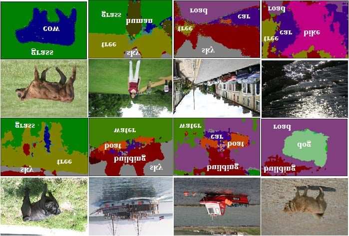
model is effective on both types of classifiers; (3) using Figure 4. The first and the fifth column displays some test images from the Weiz-
mann dataset [3]. Other columns show probability maps by the different stages of the
appearance context does not improve the result (even auto-context algorithm. The last row shows two images with the worst scores.
slightly worse); (4) The second stage of the auto-context The Weizmann dataset contains one horse in each image
usually gives the biggest improvement. and they are mostly centered. To further test the perfor-
Fig. (2) gives the procedures of the auto-context algo- mance of a trained auto-context on other images, we col-
rithm in which all the uncertainties are carried out in a prob- lect some images from Google in which there are multiple
abilistic fashion with no hard thresholding. One might think horses at various scales. Fig. (5) shows the input images and
that if the previous classifier has already made a firm deci- the results by auto-context. Notice that the small horse next
sion on a particular sample, then it is probably a waste to to the big one in the second figure of Fig. (5.a) is labeled as
include this sample in the next step. We design a variation the background.
to the auto-context algorithm, called auto-context-th which
is similar to auto-context. The only difference is that if any
pixel for i for any label k if p(yi = k|X) ≥ th where th is a
threshold, then this pixel will not be used in the next round
of training. The training time of auto-context-th does appear
to be less, but the performance is slightly worse than auto-
context. Fig. (3.b) gives the full precision-recall curves for (a) (b)
Figure 5. The first row in (a) shows some images searched by Google by typing
various algorithms. The final version of PBT based auto- key word “horses”. The second row displays the final probability map by the auto-
context achieves the best result. It significantly outperforms context algorithm trained on the Weizmann dataset [3]. (b) is the confusion matrix
on the test images from the Berkeley human body dataset [13]. The head, main body,
the CRFs model based algorithm (shown as L+M (Ren et left thigh and right thigh can be mostly detected correctly.
al.)) in Fig. (3.b) and it also shows improvement than hybrid 3.2. Human body configuration
model algorithm [11]. Training takes about half a day for To further illustrate the effectiveness of the auto-context
auto-context using cascade and a couple of days for auto- algorithm, we apply it on another problem, human body
context using PBT, with both having 5 stage of classifiers. configuration. Each body part is assigned with a label.This is now a multi-class labeling problem rather than
foreground-background segregation. As stated before, PBT
based auto-context algorithm treats two-class and multi-
class problem in an identical way. We collect around 130
images for training, and use the same set of features as in the
horse segmentation problem on image patch of size 21 × 21
(designing some specific features for this task might further
improve our result).
Fig. (6) shows the results at different stages of the auto-
context on the test images in [13]. Fig. (5.b) gives the con-
fusion matrix. As we can see, the main body, the head, the
left thigh, the right thigh and the feet can be labeled ro-
bustly in most cases. The arms appear to be confused with Figure 6. The first row displays some test images. The second, third and forth
the main body and the background. The speed on these row shows the classification map by the first, third and fifth stage of the trained auto-
test images are about the same as in the horse segmenta- context algorithm.
tion case. The existing algorithms in the problem often shows some results and the confusion matrix. The results
have a pre-segmentation stage [13, 24], which is prone to by auto-context are the marginal probabilities for each pixel
errors by the low-level segmentation algorithms. For exam- belonging to a specific class. We simply assign the label
ple, the procedures described by [13, 24] can merge seg- with the highest probability to each pixel. The accuracy by
mented regions into big ones but can not break them. This the first stage of auto-context, classification method PBT
may cause problem where there is no clear boundary be- only, achieves 50.4%. The overall pixel-wise accuracy by 4
tween the parts. The auto-context algorithm computes the layers of auto-context is 74.5% which is better than 72.2%
posterior marginals for each pixel directly. reported in [19]. However, a careful reading at the confu-
We illustrate our algorithm on gray scale images, and sion matrices by both the algorithms shows that our result
color images used in [13]. The results are better than is more consistent and the mistakes made are more “rea-
those shown in [24] in which a BP algorithm was imple- sonable”. For example, boat is mostly confused with car
mented. BP computes the marginals by propagating mes- and building whereas boat was mis-classified to many other
sages through local connected neighbors, whereas auto- classes in [19] such as water, bike, and tree.
context can take long-range context information directly. Our algorithm is more general and easier to imple-
This results in significant speed improvement. Similar to ment. The speed reported in [19] was 3 minutes per image
the argument made in the horse segmentation case, our al- whereas ours is around 70 seconds. Notice that the classifi-
gorithm is more general than [13, 24]. However, a thorough cation results are a bit scattered. Another level of algorithm
comparison of the auto-context algorithm with the state of to enforce region-based consistency is still needed. With a
art algorithms (BP, Graph-Cuts, CRFs), in terms of both post-processing stage to encourage the neighboring pixels
quality and speed, remains as future research. to have the same lable, the accuracy improves to 77.7%.
Further procedures are still required to explicitly extract Y ∗ = arg min − log p(yi |X) + α δ(yi = yj ),
the body parts since the auto-context algorithm only outputs i (i,j)
probability maps. This is probably the place where more ex-
plicit shape information can be used in the Bayesian frame- where α = 2.0 for the results in this paper.
work. It is noted that almost all the algorithms we compare
to, on the horse segmentation, human body configuration,
3.3. Scene parsing/labeling and scene labeling use the context or high-level informa-
We also applied our algorithm on the task of scene pars-
tion. CRF models are indeed context based. A direct com-
ing/region labeling. We used the MSRC dataset [19] in
parison to the algorithms reported on the MSRC dataset is
which there are 591 images with 21 types of objects manu-
given in table (1). [16] gave the accuracy measure on seg-
ally segmented and labeled (there are two additional types
mented regions rather than pixels with a score 68.4%. Using
in the new dataset). There is a nuisance category labeled as
auto-context with a post-processing achieves 77.7%.
0. The setting for this task is similar as before, and the only
Algorithm TextonBoost [19] [29] Auto-Context AC+post
difference is that we use color images in this case. Shot- Accuracy 72.2% 75.1% 74.5% 77.7%
ton et al. did not have the background model to learn the Table 1. Comparison to other algorithms on the MSRC dataset. AC+post refers to
regions of 0 label, whereas it is not a problem in our case. the result by auto-context with a post-processing for smoothing and the post process-
ing takes about 0.1 second.
However, to obtain a direct comparison to their result, we 3.4. Conclusions
also exclude the 0 label both in training and testing. We use In this paper, we have introduced an auto-context algo-
the identical training and testing images as in [19]. Fig. (7) rithm to learn a unified low-level and context model. WeBu Gs Tr Co Sp Sk Ap W Fc Ca Bi Fl Sn Bi Bk Ch Rd Ct Dg Bd Bt
Building 69 1 5 0 0 1 1 3 1 1 2 2 1 1 5 0 4 1 0 2 0
Grass 0 96 1 1 1 0 0 1 0 0 0 0 0 0 0 0 0 0 0 0 0
Tree 3 5 87 0 0 1 0 1 0 0 1 1 0 0 0 0 0 0 0 0 0
Cow 0 5 1 78 1 0 0 0 1 0 0 0 1 0 0 0 0 1 5 7 0
Sheep 1 5 3 3 80 0 0 0 0 0 0 0 0 2 0 3 2 0 0 0 0
Sky 3 0 0 0 0 95 0 1 0 0 0 0 0 0 0 0 0 0 0 0 0
Airplane 11 2 2 0 0 1 83 0 0 0 0 0 0 0 0 0 0 0 0 0 0
Water 5 5 2 0 0 2 0 67 0 3 3 0 0 1 0 0 9 0 0 1 2
Face 1 0 0 1 0 0 0 0 84 0 0 0 0 0 1 0 0 0 1 10 0
Car 14 0 1 0 0 2 3 1 0 70 0 0 1 1 1 0 4 0 0 1 2
Bike 12 0 2 0 0 0 0 1 0 1 79 0 0 0 0 0 2 0 0 2 0
Flower 1 1 2 7 2 0 0 1 3 0 0 47 0 3 17 0 0 1 1 12 0
Sign 34 0 1 0 0 0 0 0 0 0 0 0 61 0 2 0 1 1 0 0 0
Bird 9 7 3 5 10 3 0 13 1 6 0 0 0 30 0 1 2 2 6 1 0
Book 8 1 1 0 0 0 0 0 1 0 0 3 0 0 80 2 1 0 0 2 0
Chair 25 2 8 1 0 0 0 1 3 0 4 2 0 0 4 45 1 1 0 2 0
Road 11 0 1 0 0 1 0 6 0 1 0 0 0 0 0 0 78 0 0 1 0
Cat 1 0 4 0 0 0 0 11 2 0 0 0 0 4 0 1 3 68 5 0 0
Dog 4 2 5 4 3 0 0 2 7 0 0 0 0 9 0 1 3 5 52 2 0
Body 6 1 1 2 0 0 0 1 5 0 0 1 1 2 5 1 2 3 2 67 0
Boat 28 0 0 0 0 1 3 15 0 13 9 0 0 1 0 0 2 0 0 2 27
(a) (b)
Figure 7. (a) shows some difficult test images (same as shown in [19]) and a couple of typical ones, with their corresponding classified labels. (b) displays the legend and
confusion matrix. The overall pixel-wise accuracy is 74.5%. The result by PBT only achieves 50.4%. The number reported in [19] was 72.2%, and using auto-context with a
post-processing stage achieves 77.7%.
target the posterior distribution directly, and thus, the test [5] Y. Freund and R. E. Schapire, “A Decision-theoretic Generalization of On-line
Learning And An Application to Boosting”, J. of Comp. and Sys. Sci., 55(1),
phase shares the same procedures as those in the training. 1997.
The auto-context algorithm selects and fuses a large number [6] S. Geman and D. Geman, “Stochastic Relaxation, Gibbs Distributions, and the
Bayesian Restoration of Images,” IEEE Trans. PAMI, vol. 6, pp. 721-741, Nov.
supporting contexts which allow it to perform rapid mes- 1984.
sage propagation. We introduce iterative procedures into [7] X. He, R. Zemel, and M. Carreira-Perpinan “Multiscale conditional random
fields for image labelling”, Proc. of CVPR, June, 2004.
the traditional classification algorithms to refine the classi- [8] D. Hoiem, A. Efros, and M. Hebert, “Putting Objects in Perspective”, Proc. of
fication results by taking effective context information. CVPR, 2006.
[9] S. Kumar and M. Hebert, “Discriminative random fields: a discriminative frame-
The proposed algorithm is very general. Under nearly a work for contextual interaction in classification”, ICCV, 2003.
same set of parameters, we illustrate the auto-context algo- [10] S. Kumar and M. Hebert, “A Hierarchical Field Framework for Unified
Context-Based Classification”, Proc. of ICCV, 2005.
rithm on three challenging vision tasks. The results show [11] A. Levin and Y. Weiss, “Learning to combine bottom-up and top-down Seg-
to significantly improve the results by patch-based classi- mentation”, Proc. of ECCV, 2006.
[12] J. Li, A. Najmi, and R.M. Gray, “Image Classification by a Two-Dimensional
fication algorithms and demonstrate improved results over Hidden Markov Model”, IEEE Trans. on Sig. Proc., vol. 48, no. 2, pp. 517-533,
almost all the existing algorithms using CRFs and BP. It 1989.
typically takes about 30 ∼ 70 seconds to run the algorithm [13] G. Mori, X. Ren, A. Efros, and J. Malik, “Recovering Human Body Configura-
tions: Combining Segmentation and Recognition”, Proc. of CVPR, June, 2004.
of size around 300 × 200. However, a full scale of com- [14] J.R. Quinlan, “Improved use of continuous attributes in C4.5”, J. of Art. Intell.
Res., 4, pp. 77-90, 1996.
parison with various choices of the algorithm, like that con- [15] J. Pearl, “Probabilistic reasoning in intelligent systems: networks of plausible
ducted in [21], is needed. The scope of the auto-context inference”, Morgan Kaufmann, 1988.
model goes beyond vision applications and it can be ap- [16] A. Rabinovich, A. Vedaldi, C. Galleguillos, E. Wiewiora, and S. Belongie “Ob-
jects in Context”, Proc. of ICCV, 2007.
plied in other problems of multi-variate labeling in machine [17] X. Ren, C. Fowlkes, and J. Malik, “Cue integration in figure/ground labeling”,
learning and AI. Proc. of NIPS, 2005.
[18] S. Savarese, J. Winn and A. Criminisi, “Discriminative Object Class Models of
The limitations for the auto-context model are: (1) the Appearance and Shape by Correlatons”, Proc. of CVPR, June 2006.
[19] J. Shotton, J. Winn, C. Rother, and A. Criminisi, “TextonBoost: Joint App.,
features on the context information are still somewhat lim- Shape and Context Modeling for MultiClass Object Recognition and Segmenta-
ited and more explicit shape information is still required; tion”, Proc. of ECCV, 2006.
[20] A. Singhal, J. Luo, and W. Zhu, “Probabilistic spatial context models for scene
(2) different auto-context models need to be trained for dif- content understanding”, Proc. of CVPR, June, 2003.
ferent applications; (3) the training time takes a bit long (a [21] R. Szeliski, R. Zabih, D. Scharstein, O. Veksler, V. Kolmogorov, A. Agarwala,
M. Tappen, and C. Rother, “A Comparative Study of Energy Minimization Meth-
few days) for the scene parsing. ods for Markov Random Fields”, Proc. of ECCV, 2006.
Acknowledgments ZT is funded by NIH Grant U54 [22] A. Torralba, K. P. Murphy, and W. T. Freeman, “Contextual Models for Object
Detection Using Boosted Random Fields”, Proc. of NIPS, 2004.
RR021813 entitled Center for Computational Biology. We [23] Z. Tu, “Probabilistic boosting tree: Learning discriminative models for classi-
thank Yingnian Wu for many stimulating discussions. fication, recognition, and clustering”, Proc. of ICCV, 2005.
[24] Z. Tu, “An Integrated Frmework for Image Segmentation and Perceptual
Grouping”, Proc. of ICCV, Oct., Beijing, 2005.
[25] Z. Tu, X. Chen, A. Yuille, and S.C. Zhu, “Image parsing: unifying segmenta-
References tion, detection, and object recognition”, IJCV, 2005.
[26] S. Zheng, Z. Tu, and A. Yuille, “Detecting Object Boundaries Using Low-,
[1] S. Avidan, “SpatialBoost: Adding Spatial Reasoning to AdaBoost”, Proc. of Mid-, and High-Level Information”, Proc. of CVPR, June, 2007.
ECCV, 2006. [27] V. Vapnik, “Statistical Learning Theory”, Wiley-Interscience, New York, 1998.
[2] S. Belongie, J. Malik, and J. Puzicha, “Shape Matching and Object Recognition [28] L. Wolf and S. Bileschi, “A Critical View of Context”, Int’l J. on Com. Vis.,
Using Shape Contexts”, IEEE Trans. on PAMI, 24(4):509-522, April 2002. 2006.
[3] E. Borenstein, E. Sharon and S. Ullman, “Combining top-down and bottom-up [29] L. Yang, P. Meer, and D. J. Foran, “Multiple Class Segmentation Using A Uni-
segmentation”, Proc. IEEE workshop on Perc. Org. in Com. Vis., June 2004 fied Framework over Mean-Shift Patches”, Proc. of CVPR, June, 2007.
[30] J. Yedidia, W. Freeman, and Y. Weiss, “Generalized Belief Propagation”, NIPS,
[4] J. Friedman, T. Hastie and R. Tibshirani, “Additive logistic regression: a statisti- 2000.
cal view of boosting”, Ann. stat., vol. 28, no. 2, pp. 227-407, 2000.You can also read