Automatic Recall Machines: Internal Replay, Continual Learning and the Brain
←
→
Page content transcription
If your browser does not render page correctly, please read the page content below
Automatic Recall Machines:
                                             Internal Replay, Continual Learning and the Brain

                                                            Xu Ji1* , João Henriques1 , Tinne Tuytelaars2 , Andrea Vedaldi1
                                                                               1
                                                                                   VGG, University of Oxford
                                                                                        2
                                                                                          KU Leuven
arXiv:2006.12323v2 [cs.LG] 15 Jul 2020

                                                                                         Abstract

                                                    Replay in neural networks involves training on sequential data with memorized sam-
                                                    ples, which counteracts forgetting of previous behavior caused by non-stationarity.
                                                    We present a method where these auxiliary samples are generated on the fly, given
                                                    only the model that is being trained for the assessed objective, without extraneous
                                                    buffers or generator networks. Instead the implicit memory of learned samples
                                                    within the assessed model itself is exploited. Furthermore, whereas existing work
                                                    focuses on reinforcing the full seen data distribution, we show that optimizing
                                                    for not forgetting calls for the generation of samples that are specialized to each
                                                    real training batch, which is more efficient and scalable. We consider high-level
                                                    parallels with the brain, notably the use of a single model for inference and recall,
                                                    the dependency of recalled samples on the current environment batch, top-down
                                                    modulation of activations and learning, abstract recall, and the dependency between
                                                    the degree to which a task is learned and the degree to which it is recalled. These
                                                    characteristics emerge naturally from the method without being controlled for.

                                         1   Introduction
                                         The ability to learn effectively from sequential or non-stationary data remains a fundamental difference
                                         between human brains and artificial neural networks. The development of biological brains is impaired
                                         when the environment changes too fast [Wood, 2016]. On the other hand, it has long been observed
                                         that artificial neural networks catastrophically forget previously learned behavior when data is
                                         presented in a sequential manner [McCloskey and Cohen, 1989]. In other words, while biological
                                         learning favors datastreams that focus on one task at a time, the effectiveness of stochastic gradient
                                         descent depends on the opposite quality of exposure to all tasks within a small temporal window.
                                         The retention of learned behavior in neural networks can be increased with experience replay, enforced
                                         non-distributedness, or parameter-level regularization. Of these, replay is perhaps the most promising
                                         approach. Parameter-level regularization has been shown to underperform [Chaudhry et al., 2019,
                                         van de Ven and Tolias, 2019], likely due to restricting change with excessive stringency [Ramapuram
                                         et al., 2020]. Non-distributed representations limit parameter sharing a priori, preventing interference
                                         but sacrificing on memory efficiency and transfer [French, 1991, Bengio et al., 2013].
                                         Replay, where training is augmented with auxiliary batches intended to capture previously seen
                                         data [Robins, 1995], avoids both these issues as it allows for constraints to be imposed at functional
                                         level over a distributed representation. However, existing work generally uses buffers or generator
                                         networks to memorize the seen data [Chaudhry et al., 2019, Shin et al., 2017]. Buffers are memory
                                         inefficient, and generator networks have proved difficult to train for natural images given only
                                         sequential data [Lesort et al., 2019a, Aljundi et al., 2019a]. In both cases it is also inconvenient to
                                             *
                                                 Correspondence to xuji@robots.ox.ac.uk.

                                         Preprint. Under review.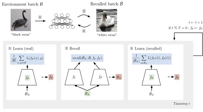
Figure 1: Automatic Recall Machines. The model trains on real B while generating and reinforcing
maximally interfered B̂ from its implicit memory. In each stage, the model or recalled samples (green)
are optimized for objective (blue) and updated (red). The change in predictions between old fθ and
new fθ0 is maximised by recall (eq. (9)). Reinforcing the resulting maximally interfered B̂X with old
outputs from fθ optimally minimizes forgetting of fθ0 , because in theory if the maximal divergence
between old and new non-local behavior is 0, then all such divergences are 0. Thus training on B
updates local behavior while training on B̂ protects behavior in the rest of input space.

require additional memory for data memorization, especially as the model being trained for directly
pertinent tasks already has an implicit memory of past training samples.
The goal of this work, Automatic Recall Machines (ARM), is to optimally exploit the implicit memory
in the tasks model for not forgetting, by using its parameters for both inference and generation (fig. 1).
For each real batch of sequential data, an auxiliary batch is optimized such that training on the latter
minimises model forgetting. Instead of attempting to reproduce the full seen data distribution, we
generate specifically the optimal samples conditioned on the current real batch, which is more efficient
and scalable. Our derivation shows that these samples are the points in input space whose outputs are
maximally changed given training on the real batch. Thus we provide a formal explanation for why
training with the most dissonant related sample is optimal for not forgetting, an intuition that was
used in Aljundi et al. [2019a]. Memory reconsolidation in humans also appears to favor conflicting
experiences [Sinclair and Barense, 2018].
We use recall to refer to internally generated replay. Automatic refers to recall being a direct conse-
quence of learning on the environment. Without an initial learning step, there is no change in knowl-
edge held by the network to compensate for and thus no recall; vice-versa, environmental batches
that cause a significant change in network knowledge induce more learning from recall (eq. (7)). In
the brain, experiences associated with higher surprise and thus representational change also increase
the intensity of replay during and after the experience [Cheng and Frank, 2008, O’Neill et al., 2008].
Without external memory for memorising samples, we hypothesized that the performance of ARM
would fall in between that of naive SGD and buffered experience replay, which is currently the
method of choice for realistic settings (natural images, “class incremental”, “single-head”) [Aljundi
et al., 2019a]. On sequential CIFAR10 and MiniImageNet, we find that augmenting training with 100
recalled images produced on-the-fly is superior to using a buffer of 100 stored real images.
While we do not directly attempt to emulate the brain, it likely remains the most successful example
of learning a distributed representation from non-stationary data, and is known to make extensive use
of experience replay [Schacter et al., 2012, Skaggs and McNaughton, 1996]. Notable traits of ARM
include a common distributed representation for tasks inference and recall, top-down modulation
via backpropagation optimization of subsequent inputs, the dependency of recall on the current
environment batch, and the bilateral dependency between tasks retention and recall. Despite replaying
at input-output level, allowing protection from forgetting to be end-to-end, we show that recall has
disproportionately meaningful effects on the deeper or more abstract representations in the network.

                                                    2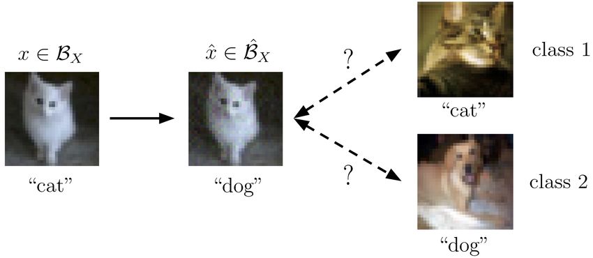
Figure 2: Real B and generated B̂ for MNIST. Images in the top row were initialized from the image
below before being optimized by recall (eq. (9)).

2     Background

In this section we discuss four underlying principles of our method.

2.1   Distributed representations

ARM trains a single neural network for all tasks, avoiding tables and task-specific parameters, as these
factors introduce enforced non-distributedness. Neural networks generally implement distributed
representations, meaning inputs are represented by overlapping patterns. Distributedness allows for
high memory efficiency [Bengio et al., 2013]; for example, n bits stores 2n patterns if overlap is
allowed and n if not. Overlap also means representations are shared between and thus optimized
across tasks, minimising redundancy from duplication. Behaviour generalises to patterns not present
in training, which is not true of non-distributed representations such as lookup tables [French, 1991].
Tables and buffers [Graves et al., 2014, Mnih et al., 2013, Chaudhry et al., 2019] are examples
of non-distributed representations, having separated cells that allow for atomic updates without
interference, but sacrificing on memory efficiency, transfer and generalisation [French, 1991, Bengio
et al., 2013]. Rather than allowing the degree of distributedness to be naturally determined from
optimization for an objective, as seen in neural network training, non-distributedness is enforced a
priori. Dynamic architectures [Rusu et al., 2016] also exploit separation, as previous parameters can
be isolated as tasks change, resulting in high memory complexity with respect to the number of tasks.
Data representation in the brain is distributed, where the number of stimuli that can be represented
increases exponentially with the number of neurons [Rolls et al., 1997]. Distributedness varies,
with for example regions implicated in fast-learning episodic memory exhibiting greater pattern
separation [Kumaran et al., 2016], but on a continuous spectrum rather than with the hard difference
seen between neural network and tabular representations.

2.2   One model for inference and recall

In ARM the invertibility of the tasks model, with its implicit memory of past training samples, is
used to generate recalled samples. Buffers or models trained for sample generation are not used.
In contrast, replay methods typically require extra memory explicitly dedicated to the auxiliary
task of sample memorisation, either in the form of buffers [Chaudhry et al., 2019, Aljundi et al.,
2019a,b, Riemer et al., 2018, Rebuffi et al., 2017, Rolnick et al., 2019] or dedicated generators [Shin
et al., 2017, Kamra et al., 2017, Lavda et al., 2018, Lesort et al., 2019b, Atkinson et al., 2018,
Kemker and Kanan, 2017]. Some parameter-level constraints (i.e. non-replay) also make use of
buffers [Lopez-Paz and Ranzato, 2017, Chaudhry et al., 2018]. Buffers being non-distributed are
relatively memory inefficient. Generator networks have so far proved difficult to train given only
non-stationary data in class-incremental settings [Lesort et al., 2019a, Aljundi et al., 2019a]. Notable
exceptions with internal generation, with key differences to our method highlighted, include Adaptive
DeepInversion [Yin et al., 2019] (generates full seen data distribution, so classes are arbitrarily pre-
selected and representativeness of batch statistics is enforced), and Replay-through-Feedback [van de
Ven et al., 2020, van de Ven and Tolias, 2018] (tasks model is overlaid with encoder of VAE,
thus shares decoder parameters in symmetric case; again, sampling is intended to represent full
distribution).
The brain also appears to share memory for inference and recall; namely the same neurons activated
during experiences are re-activated during their recall [Gelbard-Sagiv et al., 2008, Carr et al., 2011].

                                                   3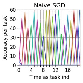
2.3   Functional rather than parameter-level constraints

A neural network can have multiple instantiations with different parameter values that execute the
same overall behavior [Williamson and Helmke, 1995]. Thus explicit constraints aimed at preventing
changes in function should be specified at the functional level, i.e. input-output, rather than at
parameter level, as noted in Ramapuram et al. [2020]. Note the two are related as functional-level
constraints are implemented as parameter-level constraints in parametric models, and parameter-level
constraints also constrain function; the difference lies in that a functional-level constraint can be
implemented as multiple parameter-level constraints but not vice-versa. The stringency of parameter
level regularization may explain its underperformance compared to replay [van de Ven and Tolias,
2019, Chaudhry et al., 2019]. ARM offers the benefit of being data-free, like some parameter level
regularizers, while being a replay method and therefore constraining at functional level.
Like ARM, LwF [Li and Hoiem, 2017] is an example of imposing functional constraints without
needing to explicitly store the seen data distribution. Unlike ARM, the replay samples are taken from
the current batch without optimization. Similarly, ARM is a form of distillation [Hinton et al., 2015].
Parameter-level methods include EWC [Kirkpatrick et al., 2017], SI [Zenke et al., 2017], GEM [Lopez-
Paz and Ranzato, 2017], A-GEM [Chaudhry et al., 2018], Meta Continual Learning [Vuorio et al.,
2018], IMM [Lee et al., 2017], Memory Aware Synapses [Aljundi et al., 2018]. These methods
generally explictly anchor either the values or gradients of parameters from excessively changing.
From an evolutionary perspective, it is overall behavior that is directly implicated for survival, as
opposed to the local behaviour of specific neurons. For example, a major influence on representations
in the brain is optimization for rewards from tasks [Miller and Cohen, 2001].

2.4   Conditionality of recall and top-down modulation

In ARM, recalled samples are optimized given model snapshots separated by training on the current
real batch, and are thus conditioned on the latter. Thus we avoid the replay-all-seen-tasks paradigm
that is inefficient and unsustainable for large numbers of tasks. Furthermore, by generating subsequent
training inputs by backpropagation - analogous to a forward pass in the opposing direction - ARM
exhibits literal top-down modulation of subsequent activations and learning within the tasks network.
Few generative replay methods (section 2.2) consider conditionality on the temporally local envi-
ronment. Rather, most aim to reproduce the full seen data distribution, with the idea that training a
network with replay simulates stationary training when replay is representative [Shin et al., 2017].
Thus randomization is used to select from buffers or choose codes or classes for decoding samples. In
contrast, Aljundi et al. [2019a] is a replay method that selectively replays based on prediction change
caused by training on the current real batch. ARM provides a theoretical argument for why this is
reasonable, as well as using internal generation instead of external buffers or generators.
Human recall is also a response conditioned on the environment as opposed to uniformly sampled
across all knowledge. Memory retrieval is conditioned on current sensory input [Carr et al., 2011].
Top-down modulation is a form of conditionality where activations representing higher-level or
downstream concepts influence the activations of lower-level or upstream representations, reversing
the bottom-up processing direction [Miller and Cohen, 2001]. It is believed that many of the cognitive
capabilities associated with the prefrontal cortex, namely various forms of reasoning, depend on its
top-down attentional modulation of other areas, conditioned on the current goal [Miller and Cohen,
2001, Russin et al., 2020]. Note that the backpropagation algorithm itself can be seen as a form of
attentional modulation of lower-level representations based on higher-level activations. However,
unlike the brain, which is highly recurrent [Kumaran et al., 2016], this top-down modulation is
truncated in that it does not yield subsequent forward pass activations nor additional learning steps.
In ARM, this is corrected as an initial learning step produces recalled inputs, yielding subsequent
activations and an additional learning step for reinforcing these activations. This allows for a chain of
inference induced by training on the environment that is longer than 1 pass over memory.

3     Automatic Recall Machines
A function parameterised by a categorical neural network fθ can be viewed as an importance-weighted
compressed store of previously seen training samples that induces inference on a much greater set.

                                                   4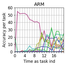
Importance corresponds to training error, as training on samples that yield no error have no impact
on the store. Given the space of outputs, Y = {1, . . . , C}, and space of inputs, for example images
X = [0, 1]3×H×W , define the knowledge of the network as its graph:
                           graph(fθ ) = {(x, y) ∈ X × Y : fθ (x) = y}.                            (1)
When training on real batch B ⊂ D from non-stationary datastream D ⊂ X × Y to obtain updated
parameters θ0 , we would like the difference between old θ and new θ0 to amount to a local change
in knowledge. θ could be the snapshot of parameters immediately preceding θ0 or, more generally,
preceding θ0 by T ≥ 1 timesteps, since we make no assumption that T = 1. Let BX and BY denote
the inputs and output targets of B. Define knowledge preservation or not forgetting as:
                         ∀x̂ ∈ X . ¬ local(x̂; B, fθ , fθ0 ) : fθ (x̂) = fθ0 (x̂)                 (2)
                    where local(x̂; B, fθ , fθ0 ) = fθ (x̂) ∈ BY ∨ fθ0 (x̂) ∈ BY .                (3)
This states that predictions for the input space should be the same for fθ and fθ0 , except inputs
mapped to the classes in B i.e. classes currently being trained. Equation (2) is satisfied iff:
                                     max          D(fθ0 (x̂), fθ (x̂)) = 0,                       (4)
                                         x̂∈X
                                  ¬ local(x̂;B,fθ ,fθ0 )

where D indicates divergence. fθ is a categorical function but in practice produces a distribution over
categories. We use the symmetric Jensen-Shannon divergence:
                                        1
                 D(fθ0 (x̂), fθ (x̂)) = · KL(fθ0 (x̂) k M ) + KL(fθ (x̂) k M ) ,                    (5)
                                        2
where M = 12 · (fθ0 (x̂) + fθ (x̂)). From eq. (4), we see that in order to suppress the forgetting of
non-local knowledge, the maximally violating input should result in no violation. Hence the best
knowledge preserving parameters in each training iteration on original batch B can be given by:
                       "                            !                                         #
                            1    X
        θ∗ = arg min                   L(fθ0 (x), y) +         sup        D(fθ0 (x̂), fθ (x̂)) ,    (6)
                 θ0        N                                   x̂∈X
                                 (x,y)∈B                               ¬ local(x̂;B,fθ ,fθ0 )

where L denotes the original tasks loss, which is cross-entropy in our experiments. This can be
approximated by:
                           "                           !                              #
                                1   X
             θ∗ = arg min                 L(fθ0 (x), y) + λ0 L(fθ0 (x̂∗ ), fθ (x̂∗ ))       (7)
                     θ0        N
                                          (x,y)∈B

                             where x̂∗ =           arg max             D(fθ0 (x̂), fθ (x̂)),                                  (8)
                                                     x̂∈X
                                              ¬ local(x̂;B,fθ ,fθ0 )

with x̂∗ being the maximally violating input. The key idea is replaying maximally violating inputs
with their old targets minimizes the maximal divergence between old model fθ and new model fθ0 ,
thus optimizing for not forgetting via eq. (4). Note no gradient exists for x̂∗ until θ0 6= θ. This
is what is meant by automatic (section 1); the optimization signal during recall (eq. (8)) and from
recall (eq. (7)) scales with the change between θ and θ0 . In practice, we fill a full replay batch of
M > 1 images, B̂X , by maximising:
recall(B̂X ; B, fθ , fθ0 ) =
"                                                                                                           !#
  1 X                                λ1      X                         λ2         X
              D(fθ0 (x̂), fθ (x̂)) +                   L(fθ (x̂), y) +                     L(fθ0 (x̂), y)        + reg(B̂X ; fθ ).
  M                                  C                                 C
     x̂∈B̂X                               y∈set(BY )                          y∈set(BY )
                                                                                                                              (9)
This is eq. (8) applied to each element of the batch with the constraint on local converted into
regularization terms. B̂Y = [fθ (x̂) : x̂ ∈ B̂X ], set(BY ) = {y : y ∈ BY } and C = | set(BY )|.
Regularization across the batch is provided by reg:
                                                                  !
                                            λ4 X
         reg(B̂X ; fθ ) = λ3 H(B̂Y ) −           L(ŷ, argmax(ŷ)) − λ5 L2(B̂X ) − λ6 T V (B̂X ),                            (10)
                                            M
                                                ŷ∈B̂Y

comprising of entropy maximisation with sharpening to prevent duplication, and L2 norm and total
variation minimization to smooth inputs [Mahendran and Vedaldi, 2015, Yin et al., 2019]. H denotes
entropy. The training procedure is summarized by algorithm 1. Standard distillation [Li and Hoiem,
2017] can be incorporated by replaying the generated batch B̂X with real batch BX (line 9).

                                                            5
Algorithm 1: Automatic Recall Machines with distillation
1 Require: randomly initialized fθ , data D, lag T , batch sizes N and M , steps S, rates η0,1 and λ0...6 .
2 θ0 = θ
3 for t ∈ [0, |D|) do
4 B = Dt
1 P
5 θ 0 = θ 0 − η0 ∇θ 0 N (x,y)∈B L(fθ 0 (x), y) . inference and learning on D
6 B̂X = BX [i0..M −1 ], i ∼ U (0, N − 1)
7 for s ∈ [0, S) do
8 B̂X = B̂X + η1 ∇B̂ recall(B̂X ; B, fθ , fθ0 ) . infer recalled samples
X
1
θ0 = θ0 − η0 ∇θ0 M +N
P
9 BX λ0 L(fθ 0 (x̂), fθ (x̂)) . learn on recalled samples
S
x̂∈B̂X
10 if (t + 1) % T = 0 then
11 θ = θ0
4 Experiments
4.1 Protocol
We use standard “class-incremental” training and evaluation protocol on sequential datasets CIFAR10-
5, MiniImageNet-20 and MNIST-5k-5 [Aljundi et al., 2019a, van de Ven and Tolias, 2019], where
suffix indicates the number of tasks. Tasks are sequential and formed by partitioning training classes
equally. Output classes are unconstrained throughout training and evaluation (single head, Farquhar
and Gal [2018]). Batch size is kept constant as it affects effective task training length. As in Aljundi
et al. [2019a], replay begins from the end of the 1st task. The update lag T is set as the number of
training iterations per task (equivalently, updating when a batch contains novel classes) [Aljundi et al.,
2019a] but we also test unit lag. Hyperparameters are selected using validation set, evaluation uses
test set, and our experiments are repeated 5 times. Hyperparameters and ablations are given in the
Appendix.
Few generative methods target class-incremental learning on natural images, which is very difficult in
our online single-pass setting. Other works generally test online generation on digits (MIR [Aljundi
et al., 2019a], GEN [Shin et al., 2017]), pre-processed features [Kemker and Kanan, 2017], or avoid
class-incremental learning by viewing entire datasets as a single task (ADI [Yin et al., 2019]).
4.2 Quantitative results
4.2.1 Comparison with buffered and generative replay
On CIFAR10 and MiniImageNet, replaying 100 recalled images with ARM outperforms experience
replay (ER) with 100 real stored images, regardless of whether MIR is used for the latter (tables 1
and 2). On MiniImageNet, replaying 100 recalled images with ARM achieves comparable perfor-
mance to ER with 500 stored real images, whilst more than halving the use of additional memory.
External generative replay methods GEN and GEN-MIR perform worse than ARM on natural
images (tables 1 and 2), despite incurring greater memory costs. This is because 3 additional
networks must be stored: old and new versions of the generator network and an old version of the
tasks network, whereas ARM uses only the latter. In particular, GEN and GEN-MIR struggled on
MiniImageNet and underperformed the naive SGD baseline. These results support the hypothesis
that for online continual learning on datasets of moderate to high complexity, obtaining meaningful
samples from the existing tasks model is easier than training a separate generator.
On MNIST, external generative experience replay does very well, but the simplicity of the dataset
allows ER methods to outperform while incurring a tenth of the memory (table 3).
4.2.2 Zero additional memory case
Unit lag is perhaps the most interesting variant of ARM from the perspective of biological plausibility,
as the old network is the current network at the start of each training iteration, hence additional memory
cost is 0. Performance drops, as using an extremely proximal version of parameters for distillation
allows for more drift. However, ARM still outperforms ADI and standard distillation (table 4).
6Method +Sample mem. +Model mem. M Accuracy Forgetting Method +Sample mem. +Model mem. M Accuracy Forgetting
#images MB #params MB #images MB #params MB
Naive SGD† 0 0 0 0 0 55.2 ± 5.0 - Naive SGD† 0 0 0 0 0 25.2 ± 4.7 -
ER 1000 3.07 0 0 10 41.3 ± 1.9 23.3 ± 2.9 ER 10000 212 0 0 10 24.8 ± 1.0 23.4 ± 1.2
ER-MIR 1000 3.07 0 0 10 47.6 ± 1.1 17.4 ± 2.1 ER-MIR 10000 212 0 0 10 25.6 ± 0.4 18.6 ± 0.7
iCarl (5 iter) 1000 3.07 0 0 - 32.4 ± 2.1 40.0 ± 1.8 ER 1000 21.2 0 0 10 6.80 ± 0.7 50.4 ± 1.8
GEM 1000 3.07 0 0 - 17.5 ± 1.6 71.7 ± 1.3 ER-MIR 1000 21.2 0 0 10 6.80 ± 0.4 51.6 ± 0.9
ER 200 0.61 0 0 10 27.5 ± 1.2 50.5 ± 2.4 ER 500 10.6 0 0 10 5.60 ± 0.4 55.2 ± 1.2
ER-MIR 200 0.61 0 0 10 29.8 ± 1.1 50.2 ± 2.0 ER-MIR 500 10.6 0 0 10 5.40 ± 0.4 55.8 ± 0.9
iCarl (5 iter) 200 0.61 0 0 - 28.6 ± 1.2 49.0 ± 2.4 ER 100 2.12 0 0 10 4.20 ± 0.4 58.6 ± 0.9
GEM 200 0.61 0 0 - 16.8 ± 1.1 73.5 ± 1.7 ER-MIR 100 2.12 0 0 10 4.00 ± 0.0 59.2 ± 0.9
ER 100 0.31 0 0 10 22.4 ± 1.1 66.2 ± 6.2
ER-MIR 100 0.31 0 0 10 23.6 ± 0.9 61.4 ± 1.8 Naive SGD 0 0 0 0 0 3.80 ± 0.2 51.2 ± 2.0
ER 10 0.03 0 0 10 18.8 ± 0.4 85.0 ± 1.1 GEN 0 0 27.1M 108 10 2.33 ± 0.3 34.3 ± 0.7
GEN-MIR 0 0 27.1M 108 20 2.00 ± 0.0 35.3 ± 0.5
Naive SGD 0 0 0 0 0 15.0 ± 3.1 69.4 ± 4.7 Distill (LwF) 0 0 1.16M 4.63 100 4.89 ± 0.2 41.6 ± 1.6
GEN 0 0 8.63M 34.5 100 15.3 ± 0.5 61.3 ± 5.1 ADI 0 0 1.16M 4.63 100 2.99 ± 0.6 8.11 ± 2.1
GEN-MIR 0 0 9.50M 38.0 40 15.3 ± 1.2 61.0 ± 1.2 ARM 0 0 1.16M 4.63 100 5.53 ± 0.8 11.9 ± 2.7
Distill (LwF) 0 0 1.09M 4.38 100 19.2 ± 0.3 60.9 ± 3.9
ADI 0 0 1.09M 4.38 100 24.8 ± 0.9 12.0 ± 4.5
ARM 0 0 1.09M 4.38 Table 2: Sequential MiniImageNet. † denotes
100 26.4 ± 1.2 8.07 ± 5.2
stationary. 3 task iterations made, as with Aljundi
Table 1: Sequential CIFAR10. † denotes station- et al. [2019a]; stationary uses 3 epochs. Chance
ary. Chance accuracy is 10.0. accuracy is 1.0.
Method +Sample mem. +Model mem. M Accuracy Forgetting Distill (LwF) ADI ARM
#images MB #params MB
Baseline (CIFAR10) 19.2 ± 0.3 24.8 ± 0.9 26.9 ± 1.1
Naive SGD† 0 0 0 0 0 87.1 ± 0.6 -
Unit lag (T = 1) 15.8 ± 2.6 14.4 ± 1.6 16.3 ± 1.8
ER 500 0.39 0 0 10 83.2 ± 1.9 13.4 ± 1.9 No distill - 20.0 ± 0.8 24.4 ± 1.7
ER-MIR 500 0.39 0 0 10 85.6 ± 2.0 10.4 ± 3.3
GEM 500 0.39 0 0 - 86.3 ± 0.1 11.2 ± 0.1
ER 50 0.04 0 0 10 62.8 ± 3.1 42.0 ± 3.7 Table 4: Testing distillation based methods:
ER-MIR 50 0.04 0 0 10 63.8 ± 4.6 40.6 ± 5.9
ER 25 0.02 0 0 10 51.6 ± 2.7 57.0 ± 3.3 unit lag and removing standard distillation.
ER-MIR 25 0.02 0 0 10 51.6 ± 2.6 56.4 ± 3.3
ER 10 0.01 0 0 10 39.2 ± 3.5 72.2 ± 4.1
Naive SGD 0 0 0 0 0 18.8 ± 0.5 95.6 ± 2.7
GEN 0 0 1.14M 4.58 40 79.3 ± 0.6 19.5 ± 0.8
GEN-MIR 0 0 1.08M 4.31 100 82.1 ± 0.3 17.0 ± 0.4
Distill (LwF) 0 0 478K 1.91 10 33.3 ± 2.5 58.0 ± 1.7
ADI 0 0 478K 1.91 10 55.4 ± 2.6 11.5 ± 5.0
ARM 0 0 478K 1.91 10 56.3 ± 2.6 21.8 ± 1.6
Table 3: Sequential MNIST. † denotes stationary. Figure 3: Optimal diversity weight (?) is neg-
Chance accuracy is 10.0. atively correlated with the number of classes.
4.2.3 Benefits of optimized selection and distributed memory
We hypothesized that the performance boost from allowing classes to be selective (ARM, *-MIR)
as opposed to random (ADI, ER, GEN) would be most obvious with a large number of classes.
The benefit of distributed (ARM, ADI, GEN-*) over non-distributed (ER-*) data stores should also
be more obvious due to the lower memory complexity of distributed representations (section 2.1).
Unfortunately, datasets with more classes are also more difficult in general, with lower baseline or
chance performance. However, we were able to verify both these hypotheses on the 100 classes
of MiniImageNet (table 2). The 2.5% accuracy boost from ARM compared to ADI equates to the
learning of 2.5 additional classes or 50% of a task. In contrast, the boost on MNIST equates to only a
tenth of a class or 5% of a task (table 3). On MiniImageNet, storing the old model costs 4.6MB but
achieves comparable performance to storing 500 images at a cost of 10.6MB.
(a) CIFAR10 (b) MiniImageNet
Figure 4: HistoryPof recalled classes throughout training for different diversity weights λ3 . Vertical
1
slices denote M x̂∈B̂X fθ (x̂) per training timestep. Current training classes (diagonal) are not
recalled due to non-locality (eq. (2)). Unseen tasks (lower triangle) are naturally avoided.
7(a) MNIST (b) CIFAR10 (c) MiniImageNet
Figure 5: Recall causes characteristic changes to learning behavior. Tasks are retained beyond their
training window and positive backwards transfer [Lopez-Paz and Ranzato, 2017] is observed.
4.3 Empirical behavior
4.3.1 Tunable diversity of recall
Varying diversity via λ3 biases recall towards sparse or dense (fig. 4a). High λ3 = 16 is optimal
for MNIST and CIFAR10 while low λ3 = 1 is optimal for MiniImageNet (fig. 3), which benefits
more from selectivity as the space of possible choices is much larger. With a low diversity weight
on CIFAR10, we observed a natural prioritization of recent classes (fig. 4a, left). This is likely
due to reduced but present forgetting causing a decrease in the discriminativeness of older class
representations relative to recent classes, resulting in the latter being highlighted in the optimization
for samples with diverging outputs. In the brain, replay is also most prevalent immediately following
an experience, and decays with time [Kudrimoti et al., 1999, Karlsson and Frank, 2009].
4.3.2 Self-reinforcing loop between task performance and recall
Naive SGD exhibits consistent and total forgetting, observable as spiking (fig. 5). In ARM, this is
notably reduced as raised accuracies remain elevated beyond the training window of the task. In
particular, we noted on every dataset that the first task was simultaneously strongly recalled (fig. 4)
and performed (fig. 5) throughout training, far beyond its own training window. The model tended to
fixate on this strongly recalled task to the detriment of performance on other tasks, which were also
not as strongly recalled. The interplay between performance and recall is expected as recall in ARM
depends entirely on the implicit memory of the tasks model; if a class is not at all retained by the
tasks model, optimization cannot recover meaningful samples for that class from the weights.
This forms a parallel with the biological brain, where increased hippocampal replay leads to increased
task performance or reward [Schuck and Niv, 2019] and vice versa [Mattar and Daw, 2018].
4.3.3 Abstract nature of recall
Images from real BX provide a favorable initialization in the optimization for maximally interfered
B̂X , since interference scales with the amount of feature overlap between them. For MNIST, the
recalled images are clearly reminiscent of the class of their associated target (fig. 2). For CIFAR10
and MiniImageNet, this is not the case, as the recalled images resemble their initialized images with
added noise. However, we found that training on recalled samples produced gradients that were
consistently more correlated with those produced from training on real images from the target class
than real images from the originator class, with strongest correlations in the highest layers (fig. 6).
Layer Corr. class 1 Corr. class 2 Layer Corr. class 1 Corr. class 2
Conv 1 0.034 ± 0.281 0.205 ± 0.254 Conv 1 0.016 ± 0.270 0.084 ± 0.275
Conv 2 0.036 ± 0.262 0.259 ± 0.214 Conv 2 0.001 ± 0.263 0.080 ± 0.261
Conv 3 0.048 ± 0.315 0.344 ± 0.234 Conv 3 -0.017 ± 0.312 0.060 ± 0.323
Conv 4 0.036 ± 0.362 0.366± 0.277 Conv 4 -0.046 ± 0.364 0.040 ± 0.388
Conv 5 0.012 ± 0.308 0.419 ± 0.210 Conv 5 -0.052 ± 0.313 0.096 ± 0.332
FC 0.002 ± 0.365 0.687 ± 0.143 FC -0.096 ± 0.351 0.137 ± 0.395
All 0.032 ± 0.278 0.355 ± 0.196 All -0.030 ± 0.279 0.071 ± 0.298
(a) Hard targets (one-hot) B̂Y (b) Soft targets B̂Y
Figure 6: Despite x̂ resembling class 1 at pixel level (a), training on x̂ produces gradients more
correlated with training on real images of class 2 than real images of class 1, with correlation being
strongest in the highest layers of the network. Hard targets (b) are considered as well as soft (c) for
fairness, as real samples use hard targets. Results shown on CIFAR10 using 1K random samples of x̂.
8This was observed across all datasets and architectures, including both convolutional ResNet and
multilayer perceptrons. Gradients within each layer were normalized for correlation, so this behavior
is not attributable to varying magnitudes. Rather, it indicates that similarities in output targets have
greater influence than similarities in input space in the computation of gradients, supporting the
argument that recalled targets are material and should be optimized rather than arbitrary (section 2.4).
Thus we found that it was not necessary for input samples to empirically resemble a particular class
for the representation of that class to be reinforced, and it was the upper or abstract layers of the
network where the most meaningful representational changes were induced by recall.
In the brain, mental imagery is thought not to propagate to the retina [Pearson et al., 2015], which has
led to the idea of replay from intermediate levels in neural networks [van de Ven et al., 2020]. However,
this requires pre-training and fixing parameters unaffected by replay, due to lack of protection from
forgetting. ARM demonstrates that replaying samples at input-output level, and thus protecting the
trained network end-to-end, has effects that can nonetheless be characterized as abstract.
4.3.4 Natural avoidance of unseen classes
ARM does not include any constraints on avoiding unseen classes. Remarkably, we discover that it
naturally does so, across diversity weights (fig. 4). This is likely because output nodes corresponding
to unseen classes have relatively undiscriminative representations, having thus far been trained not to
activate, and are therefore de-prioritized in the optimization for samples with diverging outputs.
5 Conclusion
Avoiding catastrophic forgetting in artificial neural networks naturally gives rise to recall mechanisms
reminiscent of human cognition. Internally generated, conditional replay is a promising approach
that reduces catastrophic forgetting, memory complexity, and outperforms other forms of generative
replay on natural images. Recalled samples can be deceptive at pixel level and require an analysis of
gradients to understand the relation to training on real images.
Broader Impact
This work deals with artificial neural networks internally generating imagined data. The pursuit of
human-level imagination, and cognitive abilities more generally, may allow machines to replace
humans in jobs that are currently considered protected from automation due to the creative aspect.
However, this offers potential benefits including efficiency and reducing the burden of work. The
success of neural network art and computer graphics in general has shown that not all decisions must
be consciously made by a human for creative output to have value. In addition, removing the need to
explicitly store buffered data helps algorithms overcome data protection requirements. Research at
the intersection of machine and biological intelligence has the potential to give back to neuroscience
and further the understanding of our own cognition, which is a deeply compelling objective.
Acknowledgments
With thanks to Alexei Efros for many spirited debates, and Andrew Zisserman, Philip Torr, Oliver
Groth, Christian Rupprecht and Yuki Asano for feedback. First author is funded by EPSRC.
References
Rahaf Aljundi, Francesca Babiloni, Mohamed Elhoseiny, Marcus Rohrbach, and Tinne Tuytelaars.
Memory aware synapses: Learning what (not) to forget. In Proceedings of the European Conference
on Computer Vision (ECCV), pages 139–154, 2018.
Rahaf Aljundi, Eugene Belilovsky, Tinne Tuytelaars, Laurent Charlin, Massimo Caccia, Min Lin,
and Lucas Page-Caccia. Online continual learning with maximal interfered retrieval. In Advances
in Neural Information Processing Systems, pages 11849–11860, 2019a.
Rahaf Aljundi, Min Lin, Baptiste Goujaud, and Yoshua Bengio. Gradient based sample selection
for online continual learning. In Advances in Neural Information Processing Systems, pages
11816–11825, 2019b.
9Craig Atkinson, Brendan McCane, Lech Szymanski, and Anthony Robins. Pseudo-recursal: Solving
the catastrophic forgetting problem in deep neural networks. arXiv preprint arXiv:1802.03875,
2018.
Yoshua Bengio, Aaron Courville, and Pascal Vincent. Representation learning: A review and new
perspectives. IEEE transactions on pattern analysis and machine intelligence, 35(8):1798–1828,
2013.
Margaret F Carr, Shantanu P Jadhav, and Loren M Frank. Hippocampal replay in the awake state: a
potential substrate for memory consolidation and retrieval. Nature neuroscience, 14(2):147, 2011.
Arslan Chaudhry, Marc’Aurelio Ranzato, Marcus Rohrbach, and Mohamed Elhoseiny. Efficient
lifelong learning with a-gem. arXiv preprint arXiv:1812.00420, 2018.
Arslan Chaudhry, Marcus Rohrbach, Mohamed Elhoseiny, Thalaiyasingam Ajanthan, Puneet K
Dokania, Philip HS Torr, and Marc’Aurelio Ranzato. Continual learning with tiny episodic
memories. arXiv preprint arXiv:1902.10486, 2019.
Sen Cheng and Loren M Frank. New experiences enhance coordinated neural activity in the
hippocampus. Neuron, 57(2):303–313, 2008.
Sebastian Farquhar and Yarin Gal. Towards robust evaluations of continual learning. arXiv preprint
arXiv:1805.09733, 2018.
Robert M French. Using semi-distributed representations to overcome catastrophic forgetting in
connectionist networks. 1991.
Hagar Gelbard-Sagiv, Roy Mukamel, Michal Harel, Rafael Malach, and Itzhak Fried. Internally
generated reactivation of single neurons in human hippocampus during free recall. Science, 322
(5898):96–101, 2008.
Alex Graves, Greg Wayne, and Ivo Danihelka. Neural turing machines. arXiv preprint
arXiv:1410.5401, 2014.
Geoffrey Hinton, Oriol Vinyals, and Jeff Dean. Distilling the knowledge in a neural network. arXiv
preprint arXiv:1503.02531, 2015.
Nitin Kamra, Umang Gupta, and Yan Liu. Deep generative dual memory network for continual
learning. arXiv preprint arXiv:1710.10368, 2017.
Mattias P Karlsson and Loren M Frank. Awake replay of remote experiences in the hippocampus.
Nature neuroscience, 12(7):913, 2009.
Ronald Kemker and Christopher Kanan. Fearnet: Brain-inspired model for incremental learning.
arXiv preprint arXiv:1711.10563, 2017.
James Kirkpatrick, Razvan Pascanu, Neil Rabinowitz, Joel Veness, Guillaume Desjardins, Andrei A
Rusu, Kieran Milan, John Quan, Tiago Ramalho, Agnieszka Grabska-Barwinska, et al. Overcoming
catastrophic forgetting in neural networks. Proceedings of the national academy of sciences, 114
(13):3521–3526, 2017.
Hemant S Kudrimoti, Carol A Barnes, and Bruce L McNaughton. Reactivation of hippocampal cell
assemblies: effects of behavioral state, experience, and eeg dynamics. Journal of Neuroscience, 19
(10):4090–4101, 1999.
Dharshan Kumaran, Demis Hassabis, and James L McClelland. What learning systems do intelligent
agents need? complementary learning systems theory updated. Trends in cognitive sciences, 20(7):
512–534, 2016.
Frantzeska Lavda, Jason Ramapuram, Magda Gregorova, and Alexandros Kalousis. Continual
classification learning using generative models. arXiv preprint arXiv:1810.10612, 2018.
Sang-Woo Lee, Jin-Hwa Kim, Jaehyun Jun, Jung-Woo Ha, and Byoung-Tak Zhang. Overcoming
catastrophic forgetting by incremental moment matching. In Advances in neural information
processing systems, pages 4652–4662, 2017.
10Timothée Lesort, Hugo Caselles-Dupré, Michael Garcia-Ortiz, Andrei Stoian, and David Filliat. Gen-
erative models from the perspective of continual learning. In 2019 International Joint Conference
on Neural Networks (IJCNN), pages 1–8. IEEE, 2019a.
Timothée Lesort, Alexander Gepperth, Andrei Stoian, and David Filliat. Marginal replay vs condi-
tional replay for continual learning. In International Conference on Artificial Neural Networks,
pages 466–480. Springer, 2019b.
Zhizhong Li and Derek Hoiem. Learning without forgetting. IEEE transactions on pattern analysis
and machine intelligence, 40(12):2935–2947, 2017.
David Lopez-Paz and Marc’Aurelio Ranzato. Gradient episodic memory for continual learning. In
Advances in Neural Information Processing Systems, pages 6467–6476, 2017.
Aravindh Mahendran and Andrea Vedaldi. Understanding deep image representations by inverting
them. In Proceedings of the IEEE conference on computer vision and pattern recognition, pages
5188–5196, 2015.
Marcelo G Mattar and Nathaniel D Daw. Prioritized memory access explains planning and hippocam-
pal replay. Nature neuroscience, 21(11):1609–1617, 2018.
Michael McCloskey and Neal J Cohen. Catastrophic interference in connectionist networks: The
sequential learning problem. In Psychology of learning and motivation, volume 24, pages 109–165.
Elsevier, 1989.
Earl K Miller and Jonathan D Cohen. An integrative theory of prefrontal cortex function. Annual
review of neuroscience, 24(1):167–202, 2001.
Volodymyr Mnih, Koray Kavukcuoglu, David Silver, Alex Graves, Ioannis Antonoglou, Daan
Wierstra, and Martin Riedmiller. Playing atari with deep reinforcement learning. arXiv preprint
arXiv:1312.5602, 2013.
Joseph O’Neill, Timothy J Senior, Kevin Allen, John R Huxter, and Jozsef Csicsvari. Reactivation
of experience-dependent cell assembly patterns in the hippocampus. Nature neuroscience, 11(2):
209–215, 2008.
Joel Pearson, Thomas Naselaris, Emily A Holmes, and Stephen M Kosslyn. Mental imagery:
functional mechanisms and clinical applications. Trends in cognitive sciences, 19(10):590–602,
2015.
Jason Ramapuram, Magda Gregorova, and Alexandros Kalousis. Lifelong generative modeling.
Neurocomputing, 2020.
Sylvestre-Alvise Rebuffi, Alexander Kolesnikov, Georg Sperl, and Christoph H Lampert. icarl:
Incremental classifier and representation learning. In Proceedings of the IEEE conference on
Computer Vision and Pattern Recognition, pages 2001–2010, 2017.
Matthew Riemer, Ignacio Cases, Robert Ajemian, Miao Liu, Irina Rish, Yuhai Tu, and Gerald Tesauro.
Learning to learn without forgetting by maximizing transfer and minimizing interference. arXiv
preprint arXiv:1810.11910, 2018.
Anthony Robins. Catastrophic forgetting, rehearsal and pseudorehearsal. Connection Science, 7(2):
123–146, 1995.
Edmund T Rolls, Alessandro Treves, and Martin J Tovee. The representational capacity of the
distributed encoding of information provided by populations of neurons in primate temporal visual
cortex. Experimental Brain Research, 114(1):149–162, 1997.
David Rolnick, Arun Ahuja, Jonathan Schwarz, Timothy Lillicrap, and Gregory Wayne. Experience
replay for continual learning. In Advances in Neural Information Processing Systems, pages
348–358, 2019.
Jacob Russin, Randall C O’Reilly, and Yoshua Bengio. Deep learning needs a prefrontal cortex.
2020.
11Andrei A Rusu, Neil C Rabinowitz, Guillaume Desjardins, Hubert Soyer, James Kirkpatrick, Koray
Kavukcuoglu, Razvan Pascanu, and Raia Hadsell. Progressive neural networks. arXiv preprint
arXiv:1606.04671, 2016.
Daniel L Schacter, Donna Rose Addis, Demis Hassabis, Victoria C Martin, R Nathan Spreng, and
Karl K Szpunar. The future of memory: remembering, imagining, and the brain. Neuron, 76(4):
677–694, 2012.
Nicolas W Schuck and Yael Niv. Sequential replay of nonspatial task states in the human hippocampus.
Science, 364(6447):eaaw5181, 2019.
Hanul Shin, Jung Kwon Lee, Jaehong Kim, and Jiwon Kim. Continual learning with deep generative
replay. In Advances in Neural Information Processing Systems, pages 2990–2999, 2017.
Alyssa H Sinclair and Morgan D Barense. Surprise and destabilize: prediction error influences
episodic memory reconsolidation. Learning & Memory, 25(8):369–381, 2018.
William E Skaggs and Bruce L McNaughton. Replay of neuronal firing sequences in rat hippocampus
during sleep following spatial experience. Science, 271(5257):1870–1873, 1996.
Gido M van de Ven and Andreas S Tolias. Generative replay with feedback connections as a general
strategy for continual learning. arXiv preprint arXiv:1809.10635, 2018.
Gido M van de Ven and Andreas S Tolias. Three scenarios for continual learning. arXiv preprint
arXiv:1904.07734, 2019.
Gido M van de Ven, Hava T Siegelmann, and Andreas S Tolias. Brain-like replay for continual
learning with artificial neural networks. 2020.
Risto Vuorio, Dong-Yeon Cho, Daejoong Kim, and Jiwon Kim. Meta continual learning. arXiv
preprint arXiv:1806.06928, 2018.
Robert C Williamson and Uwe Helmke. Existence and uniqueness results for neural network
approximations. IEEE Transactions on Neural Networks, 6(1):2–13, 1995.
Justin N Wood. A smoothness constraint on the development of object recognition. Cognition, 153:
140–145, 2016.
Hongxu Yin, Pavlo Molchanov, Zhizhong Li, Jose M Alvarez, Arun Mallya, Derek Hoiem, Niraj K
Jha, and Jan Kautz. Dreaming to distill: Data-free knowledge transfer via deepinversion. arXiv
preprint arXiv:1912.08795, 2019.
Friedemann Zenke, Ben Poole, and Surya Ganguli. Continual learning through synaptic intelligence.
In Proceedings of the 34th International Conference on Machine Learning-Volume 70, pages
3987–3995. JMLR. org, 2017.
12A Appendix
A.1 Datasets
Dataset Tasks Classes Classes per task #Train #Test #Val Batch size |B|
CIFAR10 5 10 2 47.5K 10K 2.5K 10
MiniImageNet 20 100 5 45.6K 12K 2.4K 10
MNIST 5 10 2 5K 10K 3K 10
Table 5: Dataset statistics.
Datasets are summarized in table 5 and follow Aljundi et al. [2019a]. Pre-processing was not used
except resizing MiniImageNet images to 84x84 as standard.
A.2 Evaluation
Average accuracy and forgetting (average drop in accuracy) were measured on a held-out test set at
the end of training on all tasks, as defined in Chaudhry et al. [2019].
Average accuracy. Let ai,j denote performance on the test set of task j after training on task i. The
average accuracy after task T is:
T
1 X
AT = aT,j . (11)
T j=1
Forgetting. Average forgetting after task T is:
T −1
1 X T
FT = fj (12)
T − 1 j=1
where fji = max al,j − ai,j . (13)
l∈{1,··· ,i−1}
A.3 Architectures and memory computations
Following Aljundi et al. [2019a], ResNet18 was used for CIFAR10 and MiniImageNet, and a multi-
layer perceptron with two hidden layers was used for MNIST. The number of parameters for each is
given in tables 1 to 3. To compute auxiliary memory usage, we assumed 3 bytes (RGB) or 1 byte
(grayscale) per pixel for sample memory, and 4 bytes (single precision floating point) per parameter
for model memory.
A.4 Hyperparameters
Dataset η0 η1 λ0 : B̂X λ0 : BX λ1 λ2 λ3 λ4 λ5 λ6 S
MNIST 0.05 25.0 1.0 1.0 1.0 0.1 16.0 0.1 1.0 1.0 10
CIFAR10 0.01 10.0 1.0 1.0 1.0 0.1 16.0 0.1 1.0 1.0 10
MiniImageNet 0.01 10.0 1.0 2.0 1.0 0.1 1.0 1.0 1.0 1.0 10
Table 6: ARM hyperparameters.
Hyperparameter values were selected based on performance on a held-out validation set. A grid search
was conducted on CIFAR10 for λ1...4 and other values were finalized by ablation. Hyperparameters
for ARM experiments in tables 1 to 3 are given in table 6. Experiments in table 4 use the same values
except λ4 = 1.0 for no distill, and an additional weight of 8.0 on D (eq. (9)) for unit lag, as we found
it was beneficial to increase the emphasis on maximal divergence in this case. Hyperparameter values
for ADI and LwF were determined in the same manner. The implementation of Aljundi et al. [2019a]
was used for ER and GEN experiments.
A.5 Code
The implementation can be found at www.github.com/xu-ji/ARM.
13A.6 Ablation
Accuracy Forgetting
Baseline (CIFAR10) 26.4 ± 1.2 8.07 ± 5.2
λ1 = 0, λ2 = 0 22.8 ± 1.8 29.1 ± 2.0
λ3 = 0 15.3 ± 1.3 4.17 ± 0.9
λ4 = 0 25.7 ± 2.0 6.69 ± 5.4
λ5 = 0 25.8 ± 1.2 6.95 ± 5.1
λ6 = 0 26.4 ± 1.7 6.36 ± 3.7
M = 150 (+50) 26.3 ± 0.9 16.5 ± 5.5
M = 50 (-50) 24.4 ± 1.2 5.71 ± 4.5
S = 20 (doubled) 25.1 ± 1.1 8.11 ± 7.2
S = 5 (halved) 24.6 ± 1.5 13.5 ± 8.4
Cross-entropy as D 24.6 ± 1.2 24.9 ± 5.2
Random noise init B̂X 16.0 ± 1.4 4.00 ± 1.1
Recall 2x per t 17.5 ± 0.6 0.57 ± 0.5
Recall 4x per t 17.4 ± 1.0 0.44 ± 0.9
Table 7: Ablation study on CIFAR10. Each result makes a change from the baseline.
The contributions of different ARM implementation details were measued with ablation (table 7).
Among the least important was image regularization; L2 norm (λ5 ) and TV minimization (λ6 ) were
added mainly for fairness with ADI, which also uses them. ARM still outperformed ADI without
them. The most important factors were initializing recalled samples from the real batch instead of
random noise, and using entropy weight (λ3 ) to minimize duplication.
M is used to denote auxiliary replay batch size. Note the material “size” for replay is not M , but
additional persistent memory size. Deliberate subsampling of the buffer (M less than size of buffer)
is used in Aljundi et al. [2019a], which prevents identical replay batches across training iterations.
This does not apply to ARM as replay images are not sampled from a fixed buffer. On CIFAR10, we
found an increase in performance up to M = 100 and diminishing returns thereafter.
Our implementation does not provide a formal guarantee of not forgetting as we only recall once
per training iteration, taking a single learning step towards minimizing divergence (algorithm 1,
line 9). We tested increasing the number of training steps from recall, looping from line 9 to line 6
in algorithm 1. This was found to lead to very strong recall of the first task throughout the training
sequence, despite high λ3 (fig. 7), and decreased overall performance (table 7). ARM typically
demonstrates a warm-up phase with fixation on the first task gradually reducing to accommodate
other tasks (fig. 5), which was suppressed in this case (fig. 7b). This result underlines the need to
consider both forgetting and accuracy, as a near eradication of forgetting (< 1% average drop in
accuracy, table 7) is not necessarily indicative of optimal overall performance. In summary, balanced
training with one recall batch per real batch was found to perform best in our experiments.
(a) (b)
Figure 7: CIFAR10 with 2 recalls per timestep t. Contrast with fig. 4a right, and fig. 5b.
14A.7 Gradients study
Layer Corr. class 1 Corr. class 2 Layer Corr. class 1 Corr. class 2
Conv 1 0.061 ± 0.316 0.246 ± 0.287 Conv 1 0.065 ± 0.319 0.212 ± 0.302
Conv 2 0.032 ± 0.274 0.282 ± 0.241 Conv 2 0.022 ± 0.273 0.262 ± 0.259
Conv 3 0.028 ± 0.326 0.414 ± 0.258 Conv 3 0.034 ± 0.315 0.381 ± 0.273
Conv 4 -0.031 ± 0.264 0.474 ± 0.198 Conv 4 -0.040 ± 0.247 0.433 ± 0.216
Conv 5 -0.181 ± 0.195 0.556 ± 0.142 Conv 5 -0.200 ± 0.190 0.505 ± 0.186
FC -0.014 ± 0.084 0.726 ± 0.084 FC -0.019 ± 0.070 0.655 ± 0.156
All -0.036 ± 0.218 0.439 ± 0.177 All -0.043 ± 0.212 0.401 ± 0.197
(a) Hard targets (one-hot) B̂Y (b) Soft targets B̂Y
Table 8: MiniImageNet.
Layer Corr. class 1 Corr. class 2 Layer Corr. class 1 Corr. class 2
FC 1 0.022 ± 0.178 0.255 ± 0.176 FC 1 0.013 ± 0.182 0.055 ± 0.196
FC 2 0.012 ± 0.168 0.325 ± 0.228 FC 2 0.015 ± 0.207 0.072 ± 0.246
FC 3 0.002 ± 0.264 0.675 ± 0.160 FC 3 0.004 ± 0.311 0.100 ± 0.293
All 0.012 ± 0.181 0.418 ± 0.181 All 0.011 ± 0.216 0.076 ± 0.233
(a) Hard targets (one-hot) B̂Y (b) Soft targets B̂Y
Table 9: MNIST.
Computing correlations for fig. 6 and tables 8 and 9 involved gradients computed from 1K real
samples and 1K recalled samples per dataset. The underlying models were taken from the end of
training and parameters were fixed. Gradients for each parameter block (i.e. weights and biases)
were linearized and normalized. 2 dot products were computed per parameter block and recalled
sample, between the gradients induced by recall and the gradients induced by training on each of 2
randomly selected real samples belonging to the recalled sample’s originator class (class 1) and target
class (class 2) respectively. Results were collected per layer and averaged over recalled samples and
parameter blocks.
15You can also read