Machine learning on DNA-encoded libraries: A new paradigm for hit-finding
←
→
Page content transcription
If your browser does not render page correctly, please read the page content below
Machine learning on DNA-encoded libraries: A new
                                            paradigm for hit-finding
                                            Kevin McCloskey1,+ , Eric A. Sigel2,3,+ , Steven Kearnes1 , Ling Xue2 , Xia Tian2 , Dennis
                                            Moccia2,4 , Diana Gikunju2 , Sana Bazzaz2 , Betty Chan2 , Matthew A. Clark2 , John W.
                                            Cuozzo2,3 , Marie-Aude Guié2 , John P. Guilinger2 , Christelle Huguet2,3 , Christopher D.
                                            Hupp2 , Anthony D. Keefe2 , Christopher J. Mulhern2,3 , Ying Zhang2 , and Patrick Riley1,*
                                            1
                                              Google Research Applied Science, Mountain View, CA, USA
arXiv:2002.02530v1 [q-bio.QM] 31 Jan 2020

                                            2
                                              X-Chem, Waltham, MA, USA
                                            3
                                              ZebiAI, Waltham, MA, USA
                                            4
                                              Cognitive Dataworks, Amesbury, MA , USA
                                            +
                                              Contributed equally to this work.
                                            *
                                              pfr@google.com

                                            ABSTRACT

                                            DNA-encoded small molecule libraries (DELs) have enabled discovery of novel inhibitors for many distinct protein targets of
                                            therapeutic value through screening of libraries with up to billions of unique small molecules. We demonstrate a new approach
                                            applying machine learning to DEL selection data by identifying active molecules from a large commercial collection and a
                                            virtual library of easily synthesizable compounds. We train models using only DEL selection data and apply automated or
                                            automatable filters with chemist review restricted to the removal of molecules with potential for instability or reactivity. We
                                            validate this approach with a large prospective study (nearly 2000 compounds tested) across three diverse protein targets:
                                            sEH (a hydrolase), ERα (a nuclear receptor), and c-KIT (a kinase). The approach is effective, with an overall hit rate of ∼30%
                                            at 30 µM and discovery of potent compounds (IC50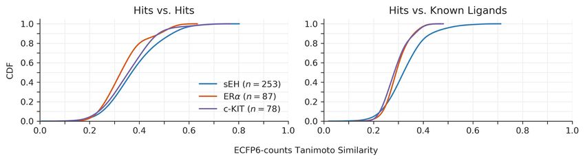
methods like random forests14, 16 ; however, the benefits of custom graph-based architectures become clear with large17 or highly
structured10 data, and DEL selection data is both.
    In this work, we demonstrate a new application of DEL selection data for discovering hits outside the compounds in the DEL
(Figure 1). First, affinity-mediated selections of the DEL under several conditions were performed with each target. Second,
the sequencing readout was processed and aggregated (see Methods). Third, a machine learning model was trained on the
aggregated selection data (using no prior off-DNA activity measurements) and used to virtually screen large libraries (∼88 M)
of easily synthesizable or inexpensive purchasable compounds. Fourth, automated diversity filters, reactive substructure filters,
and a chemist review restricted to elimination of molecules with potential instability or reactivity were applied to the top
predictions of the model. Finally, the selected compounds were tested experimentally.
    We show that graph convolutional neural network (GCNN) models16 trained with this approach generalize well to new
chemical spaces and have much stronger prospective performance than simpler baseline models. For GCNN models applied
to three different protein targets, we report hit rates for the best-performing target of 72% at 30 µM, 33% at 10 µM, and
29% at 1 µM. This is in contrast to traditional HTS (without ML), which normally reports hit rates of ∼1%18, 19 . Our results
demonstrate that this approach significantly expands the utility of DEL selection data by identifying hits in low-cost compound
libraries, producing structurally diverse starting points for both tool compound discovery and lead generation at a fraction
(∼ 25%) of the cost of typical DEL-based hit finding.

Results
Discovering potent ligands
Three therapeutic protein targets were screened: Soluble Epoxide Hydrolase (sEH) is a target for cardiovascular diseases20 ,
Tyrosine-protein kinase KIT (c-KIT) is a target for multiple pathologies including gastrointestinal stromal tumors21 , and
Estrogen Receptor Alpha (ERα) is a target for multiple pathologies including breast cancer22 .
    Two types of ML models were trained on the DEL selection data to classify compounds: Random Forest (RF)23 and
GCNN16 . The training data were preprocessed with disynthon aggregation (see Methods) to handle noise in DNA-sequencing
counts of individual library members, e.g. due to undersampling of the DEL selection output (see Figure 1). Notably, only
the DEL selection data and ML techniques described herein were used in building these models—no known ligand data were
used beyond the choice of the competitive inhibitors used in the DEL selections, and no explicit representation of the protein
targets nor 3D data were used. In fact, the authors building the GCNN models were intentionally blinded to the names and
nature of the targets at the time of model building. To cleanly assess the quality of the model predictions, we avoided subjective
selection of the most chemically attractive compounds from the predictions. To identify molecules for purchase and testing,
we started with the top predicted molecules and applied diversity, logistical, structural filters and a restricted chemist review
(see Methods). Though not automated in this experiment, this limited chemist review could be automated. All compounds
successfully acquired or synthesized were experimentally validated.
    Performance of an ML model is dependent on the data set it is trained on. In a traditional DEL screening approach, a single
selection campaign is generally sufficient for hit identification against the target of interest. To ensure this is equally true for
training predictive models, two separate DEL selections were performed months apart on sEH. This experiment showed that the
two separate training sets were equivalent with respect to model training (see Methods and Extended Data Figure 7).
    Experimental validation followed a traditional two step approach: single-point inhibition assays were run first, followed
by dose–response assays to confirm hits from the initial assays (see Methods). Dose–response potency values are reported as
the concentration required for 50% inhibition (IC50 ). The experimental hit rates and potencies are reported in Figure 2 and
cover 1885 unique compounds from two readily accessible, low-cost libraries: Mcule24 and a proprietary single reaction virtual
library (XVL; see Methods). Results from these two screening libraries have been combined for the main figures in this article.
Notably, all the experimental validations in this work are biochemical activity or ligand displacement assays, reducing the
likelihood of false positive hits that are inactive (non-binders, allosteric binders or silent binders).
    Across the three protein targets, we identified 304 ligands with better than 10 µM potency, and 165 with better than 1 µM
potency. The GCNN models achieved substantially higher hit rates and better potencies than the RF models. While the hit
rates varied across protein targets, the GCNN model still identified 78 hits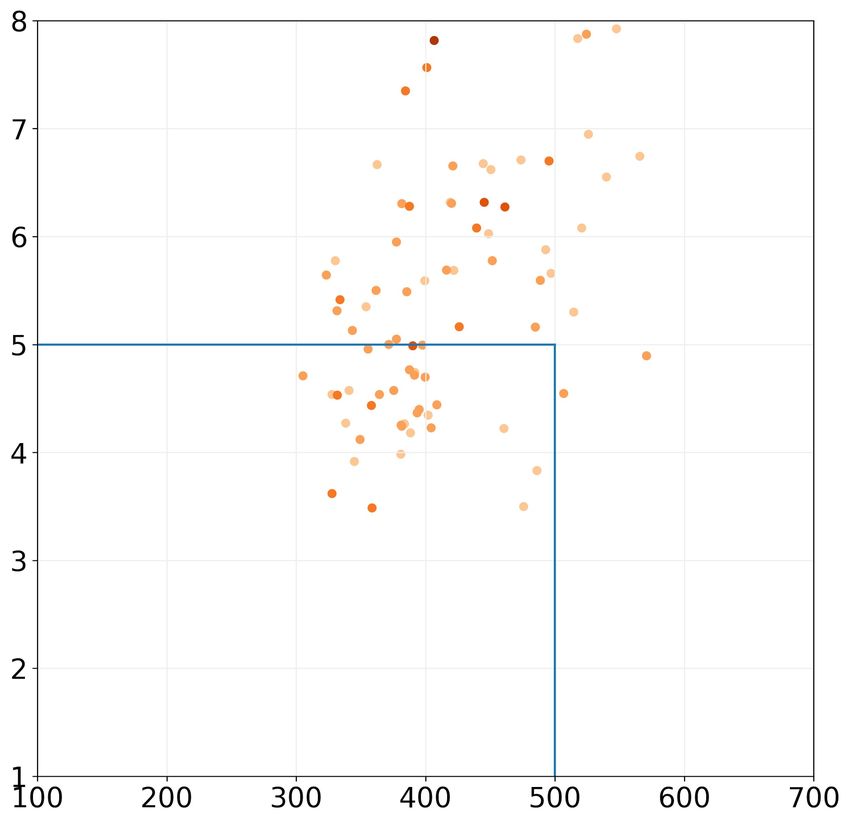
similarity search yielded no hits with detectable activity. Because this approach found zero hits, we did not repeat this baseline
for the other targets.

Analysis of confirmed hits discovered by ML
As drug discovery campaigns move from hit-finding into lead optimization, the structural diversity of the hits matters: diverse
hits act as insurance against local minima in the multi-objective lead optimization landscape26 . Despite its large size (up
to ∼1011 molecules), a DEL represents a minute fraction of the universe of small, drug-like molecules (estimated at 1033
molecules27 ), so the degree to which the ML model is accurate far from the training data is paramount. Yet—across many
applications—ML models often fail to generalize when tested on data distributions different from the training data28, 29 .
    The development of simple metrics to evaluate similarity and diversity of small molecules remains an unsolved cheminfor-
matics problem. No single metric has captured all the nuances, including differences in molecular size and domain/target-specific
knowledge of what substitutions have similar effects. The most commonly used metric is Tanimoto similarity on Extended-
Connectivity Fingerprints30 (ECFP) and their “functional class” counterpart (FCFP), see Methods for details. Another way to
analyze similarity is with Bemis–Murcko scaffolds31 , which define a central structure that can be decorated with functional
groups.
    Figure 3 depicts the cumulative hit rate and potency as a function of similarity to the nearest neighbor in the training set.
While there is evidence of a drop off in hit rate as compounds become dissimilar from the training data, the hit rates remain
useful even at less than 0.4 ECFP Tanimoto similarity to the training set (22, 28, and 5 hits with better than 30 µM potency for
sEH, ERα and c-KIT respectively); this suggests that GCNN models have the ability to generalize to unseen regions of chemical
space. Many potent hits were found far from the training set (e.g., the hit least similar to ERα training data—with ECFP
Tanimoto similarity of only 0.29 to the training set—had an IC50 of 20 nM). Extended Data Figure 2 includes similar analysis
with FCFP and produces comparable conclusions about generalization far from the DEL. Overall, there was no meaningful
correlation between the biochemical IC50 of identified hits and ECFP Tanimoto similarity to the DEL selection training set: the
largest R2 (squared regression correlation coefficient) on any target for GCNN predicted hits and RF predicted hits were 0.001
and 0.183 respectively. Extended Data Figure 4 shows distributions of similarity between confirmed hits and nearest training
set compounds, while Extended Data Table 1 highlights a selection of hits along with their nearest neighbors in the training set
(to ground these similarity numbers with specific examples). Of the Bemis–Murcko scaffolds found in the confirmed hits, only
42.7% (GCNN) and 60.8% (RF) were also contained in the training set.
    We applied diversity filtering (see Methods) in selecting compounds for testing. The final hits maintain diversity, as
illustrated by Extended Data Figure 6(b) and scaffold analysis: the 418 hits with ≤30 µM potency identified from GCNN
predictions were distributed among 370 unique Bemis–Murcko scaffolds, while the 170 hits identified from RF predictions
were distributed among 166 scaffolds.
    The confirmed hits are also structurally novel: only 2.2% (GCNN) and 3.0% (RF) of hit scaffolds were previously reported
in ChEMBL32 for these targets and Extended Data Figure 6(b) shows distributions of similarity between confirmed GCNN hits
and the nearest ChEMBL ligand (see Methods).

Discussion
Overall, we have demonstrated a new virtual screening approach that couples DEL selection data with machine learning and
automated or automatable filters to discover diverse, novel hits outside the DEL. This approach is effective on three diverse
protein targets. Because of the generalization of the ML models, practitioners have significant power in choosing a virtual
library. They could restrict screening to molecules with desirable properties, such as synthesizability, commercial availability,
presence of favored substructures, specific molecule property ranges, or dissimilarity to known ligands. In this work, we focused
on purchasable or easily-synthesizable molecules which tended to have drug-like properties. This avoids the time-consuming
and expensive process of building new chemical matter into a DEL library and performing new selections, or incorporating new
molecules into an HTS screening library. This ability to consider compounds outside of the DEL is the biggest advantage of our
approach; notably, this approach can be used at a fraction of the cost of a traditional DEL screening followup, driven primarily
by the large difference in synthesis cost (see Extended Data Table 3).
    The success of this approach is attributable to at least three factors: First, the past few years have seen the rise of more
powerful machine learning methods for many problems. For hit-finding in particular, we provide the first large scale prospective
evidence of modern graph based neural networks having a significant advantage over simpler methods. Second, DEL selection
generates both the large quantity and the high quality of data points that is essential for the training of performant machine
learning models. Lastly, large make-on-demand small molecule libraries (proprietary or commercially available) provide
a source of low-cost, structurally diverse compounds for virtual screening. Just as Lyu et al.33 showed effective use of
commercially available libraries for a computational molecular docking screen, we have shown the utility of these libraries for
machine learning driven screens.

                                                                                                                             3/19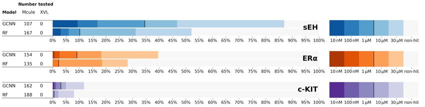
We believe the ability of a model trained on binding data to predict activity comes in part from classification criteria that
include DEL selection with a competitive binder (which may or may not be a small molecule) present in the target active site
of interest. Future application of this approach could explore areas complementary to traditional HTS (as non-ML virtual
screening has34 ), as well as integration with lead generation and optimization in combination with machine driven exploration
of chemical space (such as Zhavoronkov et al.35 ). We expect the impact of this approach to expand as DEL selections are used
to measure properties beyond competitive on-target binding; for example, some absorption, distribution, metabolism, excretion,
and toxicity (ADMET) properties may be assayable as DEL affinity-mediated screens.
    The trends of more powerful machine learning and larger, more diverse make-on-demand libraries will continue, suggesting
that the utility of the approach demonstrated here will grow over time. Further, with growth in the quality of the models and the
number of targets to which they are applied, we hope to impact later stages of the drug discovery process.

Methods
Machine learning and cheminformatics
Classification of Disynthons from Selection Data
Sequencing data for each selection condition was compiled as summed counts for all combinations of two building blocks
across all cycle combinations. For example, for a three cycle library of the form A-B-C, sums aggregating counts for the
A-B, A-C, and B-C disynthons were generated. Counts and statistics based on these counts (factoring in DNA sequencing
depth and library sizes) were used along with a cutoff to calculate a binary designation (enriched/not enriched) for each
disynthon/condition pair. The conditions included: target only, target and competitive inhibitor, and no target (matrix only)
control. Additionally, a binary indicator of promiscuity was calculated through an historic analysis of dozens of targets. First, a
promiscuity ratio for each disynthon was calculated by taking the number of protein targets selected via immobilization on any
Nickel IMAC resin where that disynthon was enriched and dividing by the total number of targets selected via immobilization
on any Nickel IMAC resin where that disynthon had been screened to date. Then, a cutoff was applied and any disynthons with
a higher ratio were considered promiscuous binders. Altogether, this procedure resulted in the assignment of each disynthon to
one of five classes: competitive hit, non-competitive hit, promiscuous binder, matrix binder, or non-hit. Competitive hits (the
“positive” class for machine learning) included disynthons that (1) were enriched in the target condition, (2) were not enriched
in the “matrix only” and “target and competitor” conditions, and (3) demonstrated a low promiscuity ratio.
Random forest models
The training data were divided into training and test sets. The number of competitive binder training examples used for the RF
models that were experimentally validated were 100 000, 87 729, and 100 000 for sEH, ERα, and c-KIT respectively. Test set
size and composition varied, with sEH, ERα, and c-KIT sets containing approximately 100 000, 10 000, 1000 positive examples,
and 190 000, 125 000, 10 000 negative examples respectively. To address memory limitations during fitting, RF models were
trained using 10 different random samples of competitive binder examples (positive examples were each included twice in
the training set) in combination with four random samples of 500 000 negative examples, resulting in a total of 40 different
training sets. Fingerprint representations for all molecules were generated using the RDKit36 implementation of 1024-bit binary
Morgan Circular Fingerprints with radius 2 (ECFP4)30 . Models were trained using the RandomForestClassifier class
in scikit-learn37 , with the following non-default hyperparameters: n_estimators=1000, min_samples_split=5,
n_jobs=6, max_features=’sqrt’, random_state=42. Performance was defined as the enrichment over random
chance of positive examples (examples predicted at ≥ 0.5) in the test set. For each target, the top performing model was used
to select predicted hits for experimental validation.
GCNN models
Architecture. The GCNN was a “weave” graph-convolutional neural network, specifically the “W2N2” variant with input
features and hyperparameters as specified by Kearnes et al.16 While the final linear layer in that work was used to make
multi-task binary classification predictions, here the final linear layer was used to make predictions on the five mutually
exclusive classes described above, trained with softmax cross entropy loss.
Cross-validation.      A k-fold cross validation scheme which split the DEL data into train, tune, and test splits was used for the
GCNN model. Each of the k folds was specified as a grouping of one or more of the DNA-encoded libraries. The groupings of
the libraries into folds were determined by plotting the first three Principal Components of the ECFP6 2048-bit binary vectors
of a random sample of disynthons from each DNA-encoded library. After plotting, the libraries that clustered visually were
grouped into the same fold, with ambiguities being resolved by grouping together libraries with similar combinatorial chemistry
reactions. k − 2 folds were then used for training each fold of the GCNN, with one tune fold reserved for training step selection,
and one test fold reserved (but ultimately not used in this study). In the c-KIT and ERα models, 10% of all the DEL selection
data stratified by each of the 5 classes (randomly sampled by hash of molecule ID) were reserved as an “ensemble holdout” set

                                                                                                                              4/19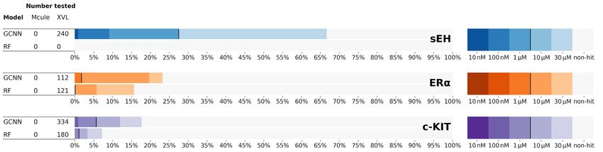
(see Extended Data Figure 3(b)). Due to third party use restrictions, for the ERα and c-KIT models a handful of productive
DNA-encoded libraries were withheld from the GCNN training data, but they were used in fitting the Random Forest model.
The number of competitive binder training examples used for the GCNN models that were experimentally validated were
355 804, 74 741 and 50 186 for the sEH, ERα, and c-KIT targets respectively.

Oversampling during training.       The vast majority of the training data is in the NON_HIT class, and the cross-validation
folds varied substantially in size. To improve training convergence time and stability of the GCNN, oversampling of the
under-represented classes and cross-validation folds was used. The mechanism of oversampling was to constrain each stochastic
gradient descent mini-batch to have equal numbers of disynthons from each class and cross-validation fold. Some fold/class
combinations had fewer than 10 disynthons and were not used. Thus, mini-batch sizes varied slightly by cross-validation fold
and protein target: the mini-batch size was the number closest to 100 that was evenly divisible by the number of fold/class
combinations with at least 10 disynthons.

Step selection and ensembling.      After training one model for each cross-validation fold, the model weights at the training
step with the maximum ROC-AUC38 for the competitive hits class on the tuning set were selected. To generate model
predictions on the Mcule and virtual library datasets for experimental validation, the median prediction for the compound
across cross-validation fold models was used.

Performance.    The average cross-validation ROC-AUC was ∼ 0.8. The ensembled model for c-KIT and ERα evaluated on
the “ensemble holdout” reached a ROC-AUC of ∼ 0.99. See Extended Data Figure 3 for details.

Compounds selected by similarity search
To further determine contribution of machine learning on our ability to select potent molecules, a parallel experiment using
Tanimoto similarity to positive training examples was conducted. Training structures were chosen from the pool of structures
used in generation of GCNN models for ERα, detailed as follows. Directed sphere exclusion39 was used with Tanimoto
similarity (ECFP6) cutoff of 0.35, ranked by the degree of enrichment in the target selection and the exemplar with highest
enrichment from each of 994 clusters was chosen. The Mcule catalog was then searched for similars to the 994 training
examples (molecules with >15 business day delivery time were excluded). Results were filtered to include compounds with
ECFP6 Tanimoto scores of ≥ 0.55. Directed sphere exclusion was again applied to the original list of Mcule similars using an
ECFP6 Tanimoto cutoff of 0.35 and ranking by maximum similarity to the training examples. From each of the resulting 114
clusters, the exemplar with the highest similarity to any input molecule was chosen. 107 compounds were received and tested.
This method produced no molecules with detectable activity.

Selection of diverse predicted compounds
Selection of compounds for order or synthesis was made for each model from those with a prediction score over a specified
cutoff (GCNN: 0.8, RF: 0.7 for Mcule and 0.5 for XVL) from either the Mcule catalog or from the XVL. Removal of duplicated
scaffolds (generated using the ’RDKit Find Murcko Scaffolds’ Knime node) was performed on some predictions, retaining
the more highly predicted structure. For GCNN Mcule selection, directed sphere exclusion clustering with ranking by model
prediction score was applied using ECFP6 Tanimoto similarity with cutoffs determined empirically to reduce the number of
molecules to hundreds or low thousands (GCNN Mcule sEH: 0.3, c-KIT: 0.5, ERα: 0.45). For both RF and GCNN Mcule
selection, hierarchical clustering was used as needed to further reduce to approximately 150 clusters. The most highly predicted
compound was selected from each cluster. For Mcule orders, compounds weighing >700 Dalton, less than a minimum MW
ranging from 190-250 Daltons (varied by target and model), and/or those with too few heavy atoms (≤ 10) were removed.
Molecules containing silicon were removed. For all orders except sEH GCNN, Mcule molecules reporting delivery times
of greater than 14 business days were excluded. To limit depletion of stocks, XVL compounds were filtered to limit the use
of any single building block; the compound with the highest prediction score for any given building block was selected. To
avoid synthesis problems, XVL compounds with reactants containing multiple reactive groups (e.g. two carboxylic acids) were
removed. For sEH XVL predictions, the top 150 remaining compounds were chosen and an additional 105 compounds were
chosen by binning prediction scores into 21 bins (size 0.05, between 0.8 and 1.0) and choosing 5 randomly from each bin. The
“Match_PAINS.vpy” script provided with Dotmatics Vortex was applied for some compound purchase and synthesis requests.
For both Mcule and XVL, an additional non-systematic visual filtering was performed by a chemist with or without the aid of
substructure searches that was restricted to removal of molecules with the potential for instability or reactivity.

Molecular similarity comparisons
Quantification of molecular structure similarity used Tanimoto similarity on extended-connectivity fingerprints30 with radius 3
(ECFP6). In this work we use a count-based representation (to better capture differences in molecular size with repeated
substructures compared to binary fingerprints) and unhashed fingerprints (to avoid hash collisions). ECFP6-counts vectors were

                                                                                                                           5/19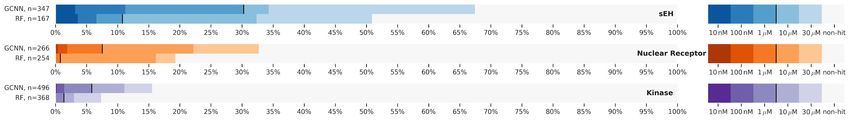
generated with RDKit36 using the GetMorganFingerprint() method with useCounts=True argument. Functional-
Class Fingerprints (FCFP) are related to ECFP, but atoms are grouped into functional classes such as “acidic”, “basic”,
“aromatic”, etc before substructures are enumerated30 . Molecules which are similar structurally but have substitutions of
similar atoms will look much more similar with FCFP than ECFP. FCFP6-counts (also with radius 3) were generated with
GetMorganFingerprint() with useCounts=True and useFeatures=True arguments. Tanimoto similarity for
two counts vectors (also commonly referred to as “1 - Jaccard Distance”) is defined as the sum of the element-wise minimum
of their counts divided by the sum of the element-wise maximum of their counts. A similarity value of 1.0 indicates identical
structures (ignoring chirality), while 0.0 means that no substructures are shared. Nearest neighbors for hits in the training data
were found using brute force exact search40 over the fingerprints.

Deep neural network architecture choice
The experimentally validated results reported in this manuscript were derived from models trained on CPUs. GCNN models
were trained to convergence on 100 CPU replicas for each fold, taking about a week for each model. Fully-connected deep
neural networks (DNN) models trained on ECFP430 bit vectors were considered for experimental validation but did not perform
as well as GCNN in cross-validation. Extended Data Figure 3 compares cross-validation performance of GCNN and DNN
models (with ReLu-activated layers of size 2000, 100), as quantified by ROC AUC38 . The cross-validation results in panel
(a) of Extended Data Figure 3 come from models not used in this study’s experimental results. They were trained on Tensor
Processing Units41 , on which the DNN and GCNN models converged in 2–3 hours, and the AUC reported is the mean AUC
from 10 models trained from scratch with different random seeds. Each of the 10 models converged 8 independently randomly
initialized sets of model weights and used the mean of the predictions from these 8 sets of weights as their overall prediction.

ChEMBL searches for published inhibitors
For sEH, a search for “epoxide hydrolase” was conducted through the ChEMBL32 website at https://www.ebi.ac.uk/
chembl/. Targets were narrowed by organism to homo sapiens, and target entries for other proteins were removed. Bioactivity
results were retrieved for the relevant target entry. Results were limited to Ki , Kd and IC50 values (i.e. percent inhibition
values were removed). All values qualified with ‘>’ or ‘≥’ were removed, as were compounds reported with Ki , Kd and IC50
>10 µM. All remaining (1607 compounds) were used for similarity comparison. Target specific searches were conducted for
ERα (’Estrogen Receptor’) and c-KIT (’KIT’); identification of published actives followed this same procedure producing
2272 and 1288 compounds respectively.

Reproducibility of training data
Two DEL selections were performed on sEH months apart. Disynthon aggregation and labeling as described above resulted in
training labels (as determined by thresholded enrichment values) that cross-predicted each other almost perfectly. We quantified
this cross-prediction performance by calculating the Area Under the Curve (AUC) of the Receiver Operator Characteristic (ROC)
curve38 . Using the first DEL selection’s positive-class enrichment values as a ranking function to predict the positive-class
binary training label of the second DEL selection achieved a ROC-AUC equal to 0.97, and predicting the first DEL selection’s
training label from the second DEL selection’s enrichment values achieved 0.99 (See Extended Data Figure 7).

Experimental
On-demand synthesis of virtual library compounds
A virtual library (XVL) comprising 83.2 M compounds was enumerated as the product of amide formation of all compatible
building blocks available in the X-Chem in-house inventory. Small libraries of compounds chosen via machine learning
prediction and filtering were synthesized in parallel on a micromole scale (about 1 µmol). The synthesis was performed in 96
well plates using a conventional synthesis protocol with DMT-MM as the coupling agent. The crude reaction mixtures were
filtered through filter plates fitted with an alumina plug. The semi-purified reaction mixtures were analyzed using LC-MS to
evaluate the reaction efficiency. The eluents were collected in 96 well receiving plates and diluted to 1 mM solution in DMSO
that was used directly for the primary biochemical assay. A small number of XVL compounds (4) identified by both GCNN
and RF models for ERα were synthesized and tested independently for each model and are reported separately in the figures
and supplementary data.

Affinity-mediated selection
All affinity-mediated selections included between 31 and 42 DEL libraries synthesized as described in Cuozzo et al.42 . For
each target, purified protein (sEH: 1 µM, c-KIT (wild type): 3 µM, ERα (wild type): 8 µM) each containing a His6 tag were
incubated in solution with DNA-encoded library (40 µM) for 1 hour in a volume of 60 µL in 1x selection buffer. 1x selection
buffer consisted of HEPES (20 mM), potassium acetate (134 mM), sodium acetate (8 mM), sodium chloride (4 M), magnesium
acetate (0.8 mM), sheared salmon sperm DNA (1 mg/mL, Invitrogen AM9680), Imidazole (5 mM), and TCEP (1 mM) at
pH 7.2. 1x selection buffer for sEH additionally included Pluronic F-127 (0.1%) and 1x selection buffer for ERα and c-KIT

                                                                                                                             6/19
additionally included Tween 20 (0.02%). For each target, an additional selection condition containing both target and 40–100
µM of a competitive inhibitor of the target was run in parallel. The competitive inhibitor was pre-incubated with the target in 1x
selection buffer for 0.5 hour prior to addition of the DNA-encoded library. For each target, an additional selection condition
containing no target was run in parallel. For each selection condition (no target, target or target with competitive inhibitor), a
separate ME200 tip (Phynexus) containing 5 µL of nickel affinity matrix was pre-washed 3 times in 200 µL of appropriate, fresh
1x selection buffer. The affinity matrix used for sEH and c-KIT was HIS-Select HF Nickel Affinity Gel (Sigma H0537) and the
affinity matrix used for ERα was cOmpleteTM His-Tag Purification Resin (Sigma 5893682001). Each selection was separately
captured with 20 passages over the appropriate ME200 tip for a total of 0.5 hour. The bound protein/library captured on the
ME200 tip was washed 8 times with 200 µL of appropriate, fresh 1x selection buffer. Bound library members were eluted by
incubating the ME200 tip with 60 µL of 1x fresh, selection buffer at 85°C for 5 min. The solution from the heat elution was
incubated with 20 passages over a fresh, pre-washed ME200 tip containing 5 µL of nickel affinity matrix to remove any eluted
protein. This selection process was run a second time using the eluate of the first selection in place of the input DNA-encoded
library and using no target, fresh target or fresh target with competitive inhibitor as appropriate. The eluate of the second round
of selection was PCR amplified in a volume of 200 µL with 5’ and 3’ primers (0.5 µM each) and 1x Platinum PCR Supermix
(Invitrogen 11306-016) with 15–25 cycles of [denaturation 94°C for 30 sec, annealing 55°C for 30 sec, and extension 72°C for
120 sec] until the double-stranded amplification products were clearly visible on an ethidium-stained 4% agarose gel. These
primers include Illumina READ1 or READ2 sequences as required for sequencing on an Illumina HiSeq 2500. PCR-amplified
selection output was then sequenced on an Illumina HiSeq 2500. Sequence read numbers (in millions) of the selections ([target,
no target control, target + competitive inhibitor]) were [93, 95, 90] for sEH, [41, 18, 39] for c-KIT, and [56, 31, 65] for ERα.
Sequence data were parsed, error-containing sequences were disregarded, amplification duplicates were removed and building
block and chemical scheme encodings were decoded and reported along with associated calculated statistical parameters.

Biochemical assays
sEH assay. The IC50 values for soluble epoxide hydrolase compounds were determined using the biochemical activity assay
described by Litovchick et al.43
c-KIT wild type assay. The IC50 values for c-KIT were determined using an ADP-Glo assay. Recombinant kinase domain
was diluted in assay buffer, 20 mM HEPES pH 7.5, 10 mM Mg acetate, 100 mM Na acetate, 1 mM DTT, 0.1% Pluronic F127,
such that the final assay concentration was 30 nM. Serially diluted test compounds were then added to the assay plate. Both
ATP and peptide substrate were then added to a final concentration of 100 µM each. The reaction was incubated for 1 hour at
room temperature and then terminated by the addition of ADP-Glo reagent and kinase detection reagents (Promega). The final
reaction volume was 12 µL. A luminescence plate reader was used to measure the signal generated by the ADP-Glo reagents
and the data points were plotted against compound concentrations.
ERα wild type assay.      Two assays were used in the course of this work reflecting availability of two different reagents.
Consistency of results between the two assays was validated with a reference compound.
    Inhibition values for ERα compounds were determined using a homogeneous time-resolved fluorescence energy transfer
assay (HTRF). Recombinant GST-tagged ERα (Thermo Fisher Scientific) was diluted into nuclear receptor assay buffer
(Thermo Fisher Scientific) containing a terbium-labeled anti-GST antibody (Thermo Fisher Scientific). Serial dilutions of test
compounds dissolved in DMSO or DMSO-only controls were dispensed into the assay plate in a volume of 120 nL and then
6 µL of GST-tagged ERα/terbium anti-GST antibody was added to the wells and incubated for 15 minutes at room temperature.
The final assay concentrations of GST-tagged ERα/antibody were 2.1 nM and 2 nM respectively. A volume of 6 µL fluorescent
ligand was then added to each well to a final concentration of 3 nM and the plates were further incubated at room temperature
for 4 hours to allow binding to reach equilibrium. HTRF signal was measured using an excitation wavelength of 337 nm and
emission wavelengths of 490 nm/520 nm on a fluorescent plate reader. The 520 nm emission signal was normalized using the
490 nm signal and plotted against compound concentrations.
    For assaying compounds chosen by the similarity search, we used a fluorescence polarization based protocol using
recombinant His-tagged ERα (in-house generated). The final assay concentrations of His-tagged ERα and fluorescent ligand
were 5 nM and 3 nM, respectively, in a total reaction volume of 12 µL. Compounds were pre-incubated with receptor for
15 minutes at room temperature prior to addition of the fluorescent ligand. After further incubation for one hour, the fluorescence
polarization signal was measured using an excitation wavelength of 485 nm and emission wavelength of 535 nm.

Assay cascade and reported potency values
In the first round of experiments for each target, single-point inhibition assays were run, and those ligands meeting the thresholds
listed in Extended Data Table 2 were re-tested with at least two 10-point dose–response curves. IC50 values were calculated
by fitting the data points to a sigmoidal curve using a four-parameter logistic model. To best utilize available budget for
dose–response curves in this study, these thresholds were decided after the single-point assays were run, solely based on the

                                                                                                                               7/19
number of molecules that would consequently receive dose–response testing. When reporting hit potencies and hit rates in
figures and text of this work, we aggregated data from both single-point inhibition assays and full dose–response curves. All
potencies reported as under 10 µM are the geometric mean of at least two validated (10-point curve) IC50 values. Dose–response
curves were validated and IC50 values excluded where the Hill slope of logistic fit < 0.5 or > 3.0 or R2 < 0.8 (when inhibition
>50% at max concentration) or R2 < 0.6 (when inhibition ≤50% at max concentration). Hits reported as 30 µM potency come
from one of the following three categories: 1) geometric mean of least two (10-point curve) IC50 values was less than 30 µM 2)
only one of the tested dose–response curves resulted in a valid IC50 (ranging from 13 nM to 28.43 µM)) or 3) single-point
inhibition assays (at 10 µM or 30 µM) showed > 50% inhibition but the compound was not re-tested with full dose–response
curves due to resource constraints.
Data availability
Chemical structures and experimentally determined potency values for tested compounds are available in a supplementary
CSV; 89 of 1992 (4.5%) have been structure-anonymized due to similarity to molecular intellectual property related to either
partnered or internal drug development programs.
Code availability
scikit-learn RandomForestClassifier was used to generate the RF predictions. A custom tensorflow implementation of the
Kearnes et. al. “W2N2” graph convolutional neural network16 was used to generate the GCNN predictions.
References
1. DiMasi, J. A., Grabowski, H. G. & Hansen, R. W. Innovation in the pharmaceutical industry: New estimates of R&D costs.
J. Heal. Econ. 47, 20–33 (2016).
2. Clark, M. A. et al. Design, synthesis and selection of DNA-encoded small-molecule libraries. Nat. Chem. Biol. 5, 647–654
(2009).
3. Goodnow, R. A. J., Dumelin, C. E. & Keefe, A. D. Dna-encoded chemistry: enabling the deeper sampling of chemical
space. Nat Rev Drug Discov 16, 131–147 (2017).
4. Harris, P. et al. DNA-encoded library screening identifies benzo[b][1,4]oxazepin-4-ones as highly potent and monoselective
receptor interacting protein 1 kinase inhibitors. J Med Chem 59, 2163–2178 (2016).
5. Machutta, C. A. et al. Prioritizing multiple therapeutic targets in parallel using automated dna-encoded library screening.
Nat. communications 8, 16081 (2017).
6. Harris, P. A. et al. Discovery of a First-in-Class receptor interacting protein 1 (RIP1) kinase specific clinical candidate
(GSK2982772) for the treatment of inflammatory diseases. J. Med. Chem. 60, 1247–1261 (2017).
7. Belyanskaya, S. L., Ding, Y., Callahan, J. F., Lazaar, A. L. & Israel, D. I. Discovering drugs with DNA-Encoded library
technology: From concept to clinic with an inhibitor of soluble epoxide hydrolase. Chembiochem 18, 837–842 (2017).
8. Satz, A. L., Hochstrasser, R. & Petersen, A. C. Analysis of current DNA encoded library screening data indicates higher
false negative rates for numerically larger libraries. ACS Comb. Sci. 19, 234–238 (2017).
9. Kuai, L., O’Keeffe, T. & Arico-Muendel, C. Randomness in DNA encoded library selection data can be modeled for more
reliable enrichment calculation. SLAS Discov 23, 405–416 (2018).
10. Gilmer, J., Schoenholz, S. S., Riley, P. F., Vinyals, O. & Dahl, G. E. Neural message passing for quantum chemistry.
In Precup, D. & Teh, Y. W. (eds.) Proceedings of the 34th International Conference on Machine Learning, vol. 70 of
Proceedings of Machine Learning Research, 1263–1272 (PMLR, International Convention Centre, Sydney, Australia,
2017).
11. Smith, J. S., Isayev, O. & Roitberg, A. E. ANI-1: an extensible neural network potential with DFT accuracy at force field
computational cost. Chem. Sci. 8, 3192–3203 (2017).
12. Schütt, K. T., Sauceda, H. E., Kindermans, P.-J., Tkatchenko, A. & Müller, K.-R. SchNet - a deep learning architecture for
molecules and materials. J. Chem. Phys. 148, 241722 (2018).
13. Li, X. et al. DeepChemStable: Chemical stability prediction with an Attention-Based graph convolution network. J. Chem.
Inf. Model. 59, 1044–1049 (2019).
14. Wu, Z. et al. MoleculeNet: a benchmark for molecular machine learning. Chem. Sci. 9, 513–530 (2018).
8/1915. Lenselink, E. B. et al. Beyond the hype: deep neural networks outperform established methods using a ChEMBL bioactivity
benchmark set. J. Cheminform. 9, 45 (2017).
16. Kearnes, S., McCloskey, K., Berndl, M., Pande, V. & Riley, P. Molecular graph convolutions: moving beyond fingerprints.
J. computer-aided molecular design 30, 595–608 (2016).
17. Ma, J., Sheridan, R. P., Liaw, A., Dahl, G. E. & Svetnik, V. Deep neural nets as a method for quantitative structure–activity
relationships. J. chemical information modeling 55, 263–274 (2015).
18. Bender, A. et al. Which aspects of hts are empirically correlated with downstream success? Curr. Opin. Drug Discov. Dev.
11, 327 (2008).
19. Clare, R. H. et al. Industrial scale high-throughput screening delivers multiple fast acting macrofilaricides. Nat. communi-
cations 10, 11 (2019).
20. Imig, J. D. & Hammock, B. D. Soluble epoxide hydrolase as a therapeutic target for cardiovascular diseases. Nat. reviews
Drug discovery 8, 794 (2009).
21. Rubin, B. P., Heinrich, M. C. & Corless, C. L. Gastrointestinal stromal tumour. The Lancet 369, 1731–1741 (2007).
22. Thomas, C. & Gustafsson, J.-Å. The different roles of er subtypes in cancer biology and therapy. Nat. Rev. Cancer 11, 597
(2011).
23. Breiman, L. Random forests. Mach. Learn. 45, 5–32 (2001).
24. Kiss, R., Sandor, M. & Szalai, F. A. http://mcule.com: a public web service for drug discovery. J. cheminformatics 4, P17
(2012).
25. Lipinski, C. A., Lombardo, F., Dominy, B. W. & Feeney, P. J. Experimental and computational approaches to estimate
solubility and permeability in drug discovery and development settings. Adv. drug delivery reviews 23, 3–25 (1997).
26. Bleicher, K. H., Böhm, H.-J., Müller, K. & Alanine, A. I. A guide to drug discovery: hit and lead generation: beyond
high-throughput screening. Nat. reviews Drug discovery 2, 369 (2003).
27. Polishchuk, P. G., Madzhidov, T. I. & Varnek, A. Estimation of the size of drug-like chemical space based on gdb-17 data.
J. computer-aided molecular design 27, 675–679 (2013).
28. Zadrozny, B. Learning and evaluating classifiers under sample selection bias. In Proceedings of the twenty-first international
conference on Machine learning, 114 (ACM, 2004).
29. Sugiyama, M. & Müller, K.-R. Input-dependent estimation of generalization error under covariate shift. Stat. & Decis. 23,
249–279 (2005).
30. Rogers, D. & Hahn, M. Extended-connectivity fingerprints. J. chemical information modeling 50, 742–754 (2010).
31. Bemis, G. W. & Murcko, M. A. The properties of known drugs. 1. molecular frameworks. J. medicinal chemistry 39,
2887–2893 (1996).
32. Gaulton, A. et al. The chembl database in 2017. Nucleic acids research 45, D945–D954 (2016).
33. Lyu, J. et al. Ultra-large library docking for discovering new chemotypes. Nature 566, 224–229 (2019).
34. Ferreira, R. S. et al. Complementarity between a docking and a high-throughput screen in discovering new cruzain
inhibitors. J. medicinal chemistry 53, 4891–4905 (2010).
35. Alex Zhavoronkov, A. A. M. S. V. V. A. A. A. V. A. V. A. T. D. A. P. M. D. K. A. A. Y. V. A. Z. R. R. S. A. Z. L. I. M. B.
A. Z. L. H. L. R. S. D. M. L. X. T. G. . A. A.-G., Yan A. Ivanenkov. Deep learning enables rapid identification of potent
ddr1 kinase inhibitors. nature biotechnology 37, 1038–1040 (2019).
36. Landrum, G. et al. Rdkit: Open-source cheminformatics (2006).
37. Pedregosa, F. et al. Scikit-learn: Machine learning in python. J. machine learning research 12, 2825–2830 (2011).
38. Fawcett, T. An introduction to roc analysis. Pattern recognition letters 27, 861–874 (2006).
39. Gobbi, A. & Lee, M.-L. Dise: directed sphere exclusion. J. chemical information computer sciences 43, 317–323 (2003).
40. Wu, X., Guo, R., Simcha, D., Dopson, D. & Kumar, S. Efficient inner product approximation in hybrid spaces. arXiv
preprint arXiv:1903.08690 (2019).
41. Jouppi, N. P. et al. In-datacenter performance analysis of a tensor processing unit. In 2017 ACM/IEEE 44th Annual
International Symposium on Computer Architecture (ISCA), 1–12 (IEEE, 2017).
9/1942. Cuozzo, J. et al. Discovery of a potent BTK inhibitor with a novel binding mode by using parallel selections with a
dna-encoded chemical library. Chembiochem 18, 864–871 (2017).
43. Litovchick, A. et al. Encoded library synthesis using chemical ligation and the discovery of seh inhibitors from a
334-million member library. Sci. reports 5, 10916 (2015).
44. Clopper, C. J. & Pearson, E. S. The use of confidence or fiducial limits illustrated in the case of the binomial. Biometrika
26, 404–413 (1934).
Acknowledgements
We acknowledge: AstraZeneca for providing reagents used in screening of both ERα and c-Kit; Zan Armstrong for help
with visual design of figures; the X-Chem Library Synthesis and Design teams for the DEL libraries; the X-Chem Scientific
Computing team for analytical tools and database capabilities; the X-Chem Lead Discovery team for input and contributions
to the X-Chem DEL tagging strategy, target screening and DEL selection analysis. Rick Wagner, Terry Loding, Allison
Olsziewski, Anna Kohlmann, Jeremy Disch and Belinda Slakman for valuable input and support during this study and the
writing of this manuscript.
Author contributions statement
P.R. and E.A.S. conceived and directed the study. K.M., S.K., E.A.S., L.X., C.J.M., Y.Z. developed the cross-validation scheme
for GCNN and/or the disynthon classification scheme used in both models. K.M. and S.K. trained the GCNN models. D.M.
and L.X. trained the RF models. E.A.S., L.X. and C.D.H. applied pre-arranged structural filtering to model predictions. X.T.
performed compound synthesis and characterization of virtual library compounds. D.G., S.B. and B.C. performed activity
assays. M.-A.G. performed statistical calculations on DEL data. A.D.K. identified suitable protein targets and selection output
datasets. J.P.G. performed DEL affinity-mediated selections. E.A.S. and M.A.C. designed the similarity search baseline
experiment. K.M., S.K., E.A.S., C.J.M., C.H. performed analysis of activity assay results. K.M., P.R., S.K., E.A.S., C.H.,
J.W.C., D.G., J.P.G., Y.Z., A.D.K. and C.J.M. wrote the paper.
Additional information
Competing interests
All authors are current or former employees of X-Chem, Inc. or Google LLC as noted in their author affiliations. X-Chem
is a biotechnology company that operates DNA-encoded library technology as part of its business. X-Chem has filed a PCT
application covering the use of DEL data with machine learning for hit identification (PCT/US2018/028050, inventors E.A.S.,
L.X., D.M., C.J.M.). Google is a technology company that sells machine learning services as part of its business. Portions of
this work are covered by issued US Patent No. 10,366,324 ("Neural Network for Processing Graph Data", P.R. is an inventor)
and a pending unpublished US patent application, both filed by Google. ZebiAI is a biotechnology company that applies
machine learning to DEL selection data as part of its business. Cognitive Dataworks is a commercial consulting and software
company.
Figures
10/19(a) Disynthon
DEL selection and
aggregation and ? ×100
positives
Chemical tag sequencing
building blocks ×13 labeling
×7
DNA tag A B C ? ×80
×6
×18
? ×9
negatives
×3
~108 unique molecules ×9
×2
? ×5
×4
~106 sequence reads ~106 labeled disynthons
(b)
Predictions on Experimental
Machine learning virtual libraries, validation of
model training (e.g., Mcule) predicted hits
ML
model
Figure 1. Schematic example of machine learning models trained on DEL data. (a) Starting with a DEL containing ∼108
unique molecules, an affinity-mediated selection is performed against the target and the DNA tags for retained molecules are
PCR-amplified and sequenced. After removal of PCR-amplification duplicates, reads for each library member are then
aggregated across shared two-cycle disynthon representations. These disynthons are labeled as positive or negative based on
calculated enrichment scores. Aggregation is performed for every possible pair of synthons; i.e., some disynthons aggregate
over the central synthon(s). The figure shows an example for a three-cycle DEL, but we also used two-cycle and four-cycle
libraries; overall, we ran selections for ∼40 libraries covering ∼1011 unique molecules. Note that additional counter-selections
may be run to provide richer labels, e.g., inclusion of a known competitive inhibitor. (b) The labeled disynthon representations
are used as training data for machine learning models. The trained models are then used to predict hits from virtual libraries or
commercially available catalogs such as Mcule. Predicted hit compounds are ordered or synthesized and tested experimentally
to confirm activity in functional assays.
Number tested
Model Mcule XVL
GCNN
RF
107
167
240
0
sEH
0% 5% 10% 15% 20% 25% 30% 35% 40% 45% 50% 55% 60% 65% 70% 75% 80% 85% 90% 95% 100% 10 nM 100 nM 1 µM 10 µM 30 µM non-hit
GCNN
RF
154
135
112
121
ER
0% 5% 10% 15% 20% 25% 30% 35% 40% 45% 50% 55% 60% 65% 70% 75% 80% 85% 90% 95% 100% 10 nM 100 nM 1 µM 10 µM 30 µM non-hit
GCNN
RF
162
188
334
180
c-KIT
0% 5% 10% 15% 20% 25% 30% 35% 40% 45% 50% 55% 60% 65% 70% 75% 80% 85% 90% 95% 100% 10 nM 100 nM 1 µM 10 µM 30 µM non-hit
Figure 2. Numbers tested along with hit rates and potencies across three therapeutic protein targets for two machine-learning
models. Compounds came from Mcule, a commercial provider, and a proprietary virtual library (XVL). Lower concentrations
correspond to more potent hits and are represented by darker colors; a black vertical line marks the 1 µM threshold in each bar
chart. Note that some compounds appeared in multiple target/model (e.g., “sEH/GCNN”) buckets, such that the number of
unique molecules is slightly smaller than the sum of the counts shown here (1885 vs. 1900).
11/19sEH ER c-KIT
100% 30 µM Clopper Pearson 95% CI 100% 30 µM Clopper Pearson 95% CI 100% 30 µM Clopper Pearson 95% CI
90% 1 µM 90% 1 µM 90% 1 µM
cumulative hit rate
80% 80% 80%
70% 70% 70%
(a) 60%
50%
60%
50%
60%
50%
40% 40% 40%
D
30%
20%
E 30%
20%
30%
20%
10% 10% 10%
10 4 10 4 10 4
10 10 10
log potency (M)
5 5 5
(b) 10 6 10 6 10 6
10 7 10 7 10 7
10 8 IC50
1-point assay
10 8 IC50
1-point assay
10 8 IC50
1-point assay
10 9 10 9 10 9
0.10
0.20
0.30
0.40
0.50
0.60
0.70
0.80
0.90
1.00
0.10
0.20
0.30
0.40
0.50
0.60
0.70
0.80
0.90
1.00
0.10
0.20
0.30
0.40
0.50
0.60
0.70
0.80
0.90
1.00
ECFP6-counts Tanimoto similarity to training set nearest neighbor
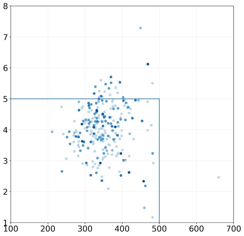
Figure 3. Cumulative hit rates of GCNN-predicted compounds (a), along with a scatter plot of hits (b), on a shared x-axis of
ECFP6-counts Tanimoto similarity of compounds to the training DELs. The cumulative hit rate plots show the hit rates for
compounds with ≤ a given (x-axis) similarity to the training set. For example, the observed sEH hit rate at 1 µM was 29.7%
(point D for sEH, 347 compounds tested), but when only considering compounds that have ≤ 0.40 similarity to the training set
nearest neighbor (point E, 36 compounds tested), the hit rate drops to 22.2%. Error bands are Clopper–Pearson intervals44 at
95% confidence.
IC50 Nearest
Target Confirmed Hit Similarity
(nM) ChEMBL Hit
sEH 1 0.39 (0.4)
sEH 2 0.44 (0.65)
ERα 8 0.26 (0.28)
ERα 20 0.2 (0.27)
c-KIT 9 0.3 (0.33)
c-KIT 21 0.23 (0.25)
Table 1. Examples of potent hits for each target. For each hit compound, we show the closest previously known ChEMBL hit
as measured by Tanimoto on ECFP6-counts fingerprints. Similarity values are given as ECFP6-counts (FCFP6-counts). A
redacted set of hits and nearest neighbors for all targets is given in the Supplementary Information.
12/19(a)
(b)
Extended Data Figure 1. Hit rates and potencies broken out by Mcule (a) and XVL (b) compounds.
13/19sEH ER c-KIT
100% 30 µM Clopper Pearson 95% CI 100% 30 µM Clopper Pearson 95% CI 100% 30 µM Clopper Pearson 95% CI
90% 1 µM 90% 1 µM 90% 1 µM
cumulative hit rate
80% 80% 80%
70% 70% 70%
(a) 60%
50%
60%
50%
60%
50%
40% 40% 40%
30% 30% 30%
20% 20% 20%
10% 10% 10%
10 4 10 4 10 4
log potency (M)
10 5 10 5 10 5
(b) 10 6 10 6 10 6
10 7 10 7 10 7
10 8 IC50
1-point assay
10 8 IC50
1-point assay
10 8 IC50
1-point assay
10 9 10 9 10 9
100% 30 µM Clopper Pearson 95% CI 100% 30 µM Clopper Pearson 95% CI 100% 30 µM Clopper Pearson 95% CI
90% 1 µM 90% 1 µM 90% 1 µM
cumulative hit rate
80% 80% 80%
70% 70% 70%
(c) 60%
50%
60%
50%
60%
50%
40% 40% 40%
30% 30% 30%
20% 20% 20%
10% 10% 10%
10 4 10 4 10 4
log potency (M)
10 5 10 5 10 5
(d) 10 6 10 6 10 6
10 7 10 7 10 7
10 8 IC50
1-point assay
10 8 IC50
1-point assay
10 8 IC50
1-point assay
10 9 10 9 10 9
100% 30 µM Clopper Pearson 95% CI 100% 30 µM Clopper Pearson 95% CI 100% 30 µM Clopper Pearson 95% CI
90% 1 µM 90% 1 µM 90% 1 µM
cumulative hit rate
80% 80% 80%
70% 70% 70%
(e) 60%
50%
60%
50%
60%
50%
40% 40% 40%
30% 30% 30%
20% 20% 20%
10% 10% 10%
10 4 10 4 10 4
log potency (M)
10 5 10 5 10 5
(f) 10 6 10 6 10 6
10 7 10 7 10 7
10 8 IC50
1-point assay
10 8 IC50
1-point assay
10 8 IC50
1-point assay
10 9 10 9 10 9
100% 30 µM 100% 30 µM 100% 30 µM
90% 1 µM 90% 1 µM 90% 1 µM
cumulative hit rate
80% Clopper Pearson 95% CI 80% Clopper Pearson 95% CI 80% Clopper Pearson 95% CI
70% 70% 70%
(g) 60%
50%
60%
50%
60%
50%
40% 40% 40%
30% 30% 30%
20% 20% 20%
10% 10% 10%
10 4 10 4 10 4
log potency (M)
10 5 10 5 10 5
(h) 10 6 10 6 10 6
10 7 10 7 10 7
10 8 IC50
1-point assay
10 8 IC50
1-point assay
10 8 IC50
1-point assay
10 9 10 9 10 9
0.10
0.20
0.30
0.40
0.50
0.60
0.70
0.80
0.90
1.00
0.10
0.20
0.30
0.40
0.50
0.60
0.70
0.80
0.90
1.00
0.10
0.20
0.30
0.40
0.50
0.60
0.70
0.80
0.90
1.00
Tanimoto similarity to training set nearest neighbor
Extended Data Figure 2. Cumulative hit rates of model-predicted compounds (a), (c), (e), (g), along with scatter plots of
hits (b), (d), (f), (h)) on a shared x-axis of Tanimoto similarity of compounds to the training DELs. GCNN-predicted
compounds in (a), (b) use ECFP6-counts fingerprints for x-axis similarity. GCNN-predicted compounds in (c), (d) use
FCFP6-counts fingerprints for x-axis similarity. RF-predicted compounds in (e), (f) use ECFP6-counts fingerprints for x-axis
similarity. RF-predicted compounds in (g), (h) use FCFP6-counts fingerprints for x-axis similarity. The cumulative hit rate
plots show the hit rates for compounds with ≤ a given (x-axis) similarity to the training set. Error bands are Clopper–Pearson
intervals44 at 95% confidence.
14/191.0
sEH 1.0
ER 1.0
c-KIT
GCNN avg=0.78, DNN avg=0.76 GCNN avg=0.83, DNN avg=0.79 GCNN avg=0.82, DNN avg=0.77
0.9 0.9 0.9
GCNN test set AUC
0.8 0.8 0.8
(a)
0.7 0.7 0.7
0.6 0.6 0.6
0.5 0.5 0.5
0.5 0.6 0.7 0.8 0.9 1.0 0.5 0.6 0.7 0.8 0.9 1.0 0.5 0.6 0.7 0.8 0.9 1.0
DNN test set AUC DNN test set AUC DNN test set AUC
1.0 1.0 1.0
0.9 0.9 0.9
0.8 0.8 0.8
GCNN AUC
(b)
0.7 0.7 0.7
0.6 0.6 0.6
tune set avg=0.81 tune set avg=0.8
tune set avg=0.77 ensemble_holdout set avg=0.96 ensemble_holdout set avg=0.96
0.5 0.5 0.5
tune set tune ensemble_holdout post_ensemble tune ensemble_holdout post_ensemble
split split
Extended Data Figure 3. Comparison of cross validation model performance, between (a) a GCNN model and a DNN
model (see Methods), and (b) on holdout sets evaluated on the models used to make experimentally validated predictions.
Extended Data Figure 4. Similarity between confirmed hits and nearest training examples from GCNN predictions. (Top
row) Distributions of ECFP6-counts Tanimoto similarity between confirmed hits and the most similar compound in the training
set. (Bottom row) Distributions of ECFP6-counts Tanimoto similarity between confirmed hits and the most similar positive
training example. In all plots, the distribution mean is indicated with a vertical black line.
15/19sEH ER⍺ c-KIT
253 / 253 73 / 87 78 / 78
(100%) (83.9%) (100%)
Crippen LogP
Molecular weight
Extended Data Figure 5. Scatter plot of molecular weight and calculated Crippen LogP for confirmed active ligands
predicted by GCNN. Blue lines indicate Lipinski "Rule of 5" thresholds. Inset in gray boxes are the portion of hits at 30 µM
that have 1 or fewer "Rule of 5" violations.
colab: https://colab.corp.google.com/drive/12l4HmCVORKvWFZV2kV1nJ7K6GZDr7Aqn#scrollTo=Avbdwc72DDMe
(a) (b)
(c) 0.24 0.32 0.49 0.55 0.64
(0.28) (0.42) (0.55) (0.68) (0.76)
Extended Data Figure 6. Similarity between confirmed GCNN hits. (a, b) Cumulative distribution functions (CDFs) of
maximum ECFP6-counts Tanimoto similarity between compounds for each target. For each compound, the maximum
similarity to (a) other hits or (b) known ligands for the same target is reported. The number of known ligands for each target is
as follows: 1607 (sEH), 2272 (ERα), 1288 (c-KIT). A redacted set of hit structures and the full set of known ligands for each
target are available as Supplementary Information. (c) Examples of hit–hit pairs for sEH are shown to illustrate similarity at a
variety of Tanimoto levels; similarity values are given as ECFP6-counts (FCFP6-counts).
16/19You can also read