Bayesian gaussian finite mixture model - Journal of Physics: Conference Series - IOPscience
←
→
Page content transcription
If your browser does not render page correctly, please read the page content below

Journal of Physics: Conference Series

PAPER • OPEN ACCESS

Bayesian gaussian finite mixture model
To cite this article: J Mirra and S Abdullah 2021 J. Phys.: Conf. Ser. 1725 012084

View the article online for updates and enhancements.

                               This content was downloaded from IP address 46.4.80.155 on 06/05/2021 at 04:51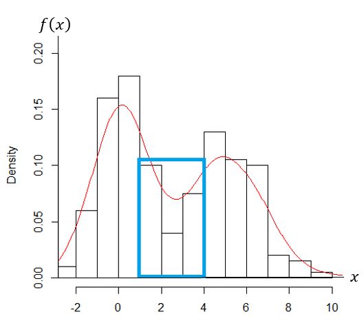
2nd BASIC 2018                                                                                                  IOP Publishing
Journal of Physics: Conference Series                         1725 (2021) 012084          doi:10.1088/1742-6596/1725/1/012084

      Bayesian gaussian finite mixture model

                         J Mirra and S Abdullah
                         Department of Mathematics, Faculty of Mathematics and Natural Sciences (FMIPA),
                         Universitas Indonesia, Depok 16424, Indonesia

                         Corresponding author’s email: sarini@sci.ui.ac.id

                         Abstract. In data analysis it is common to assume that data are generated from one population.
                         However, due to some underlying factors, data might come from several sources that should be
                         considered as several sub-populations. Partitioning methods such as k-means clustering, as well
                         as hierarchical clustering, are two commonly used methods for identifying data grouping. The
                         grouping is done based on distance between observations. We discuss alternative means of data
                         grouping, based on data distribution, known as Finite Mixture Model. Parameter estimation will
                         be done using the Bayesian approach. Incorporation of prior distribution on the parameter of
                         interest will complete data information from the sample, resulting in updated information in the
                         form of posterior distribution. Gaussian distribution is assumed for the sampling model. Markov
                         Chain Monte Carlo with Gibbs Sampling algorithm is implemented for sampling from the
                         posterior distribution. Data on wave sensitivity on monkeys’ eyes were used to illustrate the
                         method.

                         Keywords: Monte Carlo, prior distribution, posterior distribution, sampling model, simulation

      1. Introduction
      Statistical methods that are often used in data grouping include the k-means and hierarchical clustering
      method. These methods assume that data comes from one population, that is, data follows a certain
      distribution. Thus, the groupings are based solely on the distance between observations. We argue that
      this approach is not suitable for heterogeneous data. Partitioning data based on the distribution seemed
      to be more appropriate, as distribution preserve patterns in data, which is often ignored in methods that
      rely on distance measurement.
          For example, as illustrated in our simulated data displayed in figure 1, data in the region of the blue
      box will be considered as one group, since their values are close, if we are using the distance-based
      method for grouping. However, it is clearly seen that part of this data is more likely under the density
      line of the first distribution (the one with the higher density for mode), and the rest is under the density
      of the second distribution (the one with the lower density for mode). Thus, a density-based clustering is
      sought for grouping this type of data.
          Finite mixture models (FMM) [1] is flexible to model large heterogeneous data [2].
      The heterogeneity might be due to some underlying, or latent, factors that assuming data comes from
      just one population may lead to unreliable analysis results. Although the number of groups, hereafter
      will be called sub-populations, are usually unknown, in FMM it is given. Therefore, some options for
      sub-population number will be given, starting from 1, and will stop until the optimal number is reached.
      The optimal number is determined using the Goodness of Model (GoF) fit information criterion.

              Content from this work may be used under the terms of the Creative Commons Attribution 3.0 licence. Any further distribution
              of this work must maintain attribution to the author(s) and the title of the work, journal citation and DOI.
Published under licence by IOP Publishing Ltd                          1
2nd BASIC 2018 IOP Publishing
Journal of Physics: Conference Series 1725 (2021) 012084 doi:10.1088/1742-6596/1725/1/012084
Figure 1. Example of data that generated from a mixture of
two distributions. x represents the realization of the data value,
represents the density distribution of x.
While frequentist approach is common in conventional statistical parameter estimation, it relies
heavily on data quality. For example, in maximum likelihood method, the estimated parameters are
obtained by maximizing the likelihood function, which is formed by the joint distribution of the sample
data. On the other hand, Bayesian approach offers a measure of flexibility in parameter estimation [3].
By flexibility we meant that the estimated parameters are obtained not based solely on data, but also
taking into account other sources of information, such as experts’ opinions, or the results from similar
previous studies to complete the information from a data sample. This additional information is known
as prior, accommodated in the model through specification of prior distribution for the parameters of
interest. Combining the prior information and sampling model (from sample data) results in a posterior
distribution, that can be viewed as an updated information in which our inference will be based on.
Since in addition of sample data it also considers the prior information, we consider the Bayesian
approach to be more comprehensive than the frequentist approach, and shall thus implement this method
in this study. While others may argue that there is a possibility of unreliable prior information that will
eventually lead to less accurate results compared to just relying on data, under the Bayesian procedure,
the resulting posterior is optimal, considering the condition set by the prior [4]. Moreover, if the quality
of prior information is questionable, we can always set the prior distribution to be vague, known as a
flat or uninformative prior [5]; thus, the posterior will be dominated by the information from the sample
data, as in frequentist approach. This property leads to the flexibility of the Bayesian approach.
An analytic solution to the posterior distribution is often difficult to obtain. Thus, we implemented
numerical simulation through Markov Chain Monte Carlo (MCMC) with Gibbs Sampling to sample
parameters from their posterior distribution [6-8]. As an example of application of Gaussian Bayesian
FMM, we use data on the sensitivity level wave of monkeys’ eyes [9].
2. Statistical methods
2.1. Finite mixture model
Let data consists of observations on one numerical measurement, say , that is,
. Assume that data might come from sub-populations ( will be determined
22nd BASIC 2018 IOP Publishing
Journal of Physics: Conference Series 1725 (2021) 012084 doi:10.1088/1742-6596/1725/1/012084
later) with each population is represented by the density with is the parameter(s) of
sub-population , . Then, the finite mixture model is as follows:
(1)
where
is the density function,
is the weight of each sub-population, such
that
! " # # !and
is the mean parameter in each subpopulation .
This equation describes the combining of probability density function of each formed sub-population.
Each sub-population is assigned the proportion (weight) that reflects the chance of each group
representing the overall data. Assuming Gaussian distribution for the sampling model, takes the
form of a Gaussian probability density function, where the parameter may differ between sub-
populations.
According to the model, in order to assign each observation to the suitable sub-population, the
parameter needs to be estimated. Furthermore, once all the sub-populations have been formed, the
characteristics of those sub-populations must be determined, thus requiring the estimation of parameter
. Parameter estimation through Bayesian approach will be discussed in the subsequent section.
2.2. Bayesian gaussian finite mixture model
According to the sampling model in equation 1, the parameters to be estimated are the sub-population
weights and the sub-population characteristics . Thus, prior distribution as an initial information
on those parameters should be specified, namely the prior distribution. Since is the weight, it is
reasonable to choose Dirichlet distribution [10] -which can be viewed as generalization of a two-class
Bernoulli distribution for , that is
$!%&'( (2)
where ( ) )
is the hyper-parameter representing the initial belief on how to distribute all
!observations into sub-populations. The functional form of Dirichlet distribution is
,- .
* +
, where * means proportional to. We only consider the functional form, and ignore
the constant terms, due to the difficulty on estimating the combined constant terms later in the posterior
distributions (known as the normalizing constant). However, as the distributional shape is determined
by the functional form, and the solution is based on numerical simulation, this approach is acceptable.
Meanwhile, the prior for !the mean of sub-population is assumed to follow a Gaussian
distribution with mean / and variance 0/ , as the following:
<
1 7 89 :; 46
; / =
2 3456 5
(3)
<
* 89 :; 46
; / =.
5
Rewriting the sampling model in equation 1, we obtain the likelihood as the following:
> 0/
0/
(4)
@A .B- 6
+
4 ? 3 89 :; 4 6 =
32nd BASIC 2018 IOP Publishing
Journal of Physics: Conference Series 1725 (2021) 012084 doi:10.1088/1742-6596/1725/1/012084
D 6
AEF@A .B-
* . 89 C; G (5)
456
Applying the Bayes rule,
9HIJ8KLHK * 9KLHK!M!NLO8NLPHHQ
* R
we obtain the posterior distribution of and is as the following:
D @ 6
,- . AEF A .B- T
* 89 :; 46
; / =!S +
R
89 :; 6 =!S!!+
-
5 45
D @ 6
AEF A .B- T U,- .
!!!!!!! 89 :; 4 6
; / =!S
89 :; 456
=!S +
-
(6)
5
posterior for mean, posterior for proportion,
Posterior distribution for proportion follows a Dirichlet distribution, %&'M V (, and posterior
distribution for mean is a normal distribution. Samples of parameters will be drawn from the posterior
distribution using numerical approach, through MCMC with Gibbs Sampling.
2.3. Markov Chain Monte Carlo
MCMC simulation is often used in Bayesian inference, especially if the posterior distributions of the
parameters observed have a complicated form. Using MCMC will accrue to a sequence of random
sample which correlates, that is, the value of the j-th sample of , for each of its element, !, is updated
by sample from the previous iteration. The sampling procedure is using Gibbs sampling, which the
algorithm is presented below (algorithm 1).
Algorithm 1. MCMC with Gibbs Sampling.
/ / / / /
Input: Initial values for and :
!and
, and the number of iterations W.
Sampling Steps:
/ / / / / /
Sample from a complete posterior distribution of X
.
/ / / / /
Sample from a complete posterior distribution of X
.
…
/ / /
Sample
from a complete posterior distribution of
.
.
/ /
Sample from a complete posterior distribution of
.
.
/ /
Sample from a complete posterior distribution of
. X
.
…
Sample
from a complete posterior distribution of
.
. .
Repeat Sampling steps until W iterations are completed.
Output: A sequence of Y< Z[ [2nd BASIC 2018 IOP Publishing
Journal of Physics: Conference Series 1725 (2021) 012084 doi:10.1088/1742-6596/1725/1/012084
Not all samples are used for inference. The first W/ \ W samples were considered as burn-in; usually
the values are still fluctuating (not convergent). The remaining W ; W/ samples that show convergence
will be used for further analysis.
Since the number of sub population is specified when building the model, an evaluation on the fitness
of the model needs to be done. Model assessment is conducted using Akaike's Information Criterion
(AIC). The AIC for model with sub-population is,
]^_
;`abcd d V `e
(7)
where ;`abcd d is the fitted model’s deviance measuring the fitness of the model to data
(d d ) are the estimated values of , and `e
is the number of parameters to be estimated,
measuring the complexity of the model. A small value of AIC indicates fitness of the model; thus, an
optimal model is the result of a trade-off between maintaining model fitness and simplicity.
3. Results and discussion
We implemented the method on wavelength sensitivity in a monkey’s eyes [9], consists of
48 measurements. A sample of 150,000 iterations were drawn from the posterior distribution, including
50,000 first iterations as burn-in. The number of sub-populations was initially set to 2 and was increased
one at a time, then stopped when the optimum number of sub-populations is reached. The AIC for each
model was recorded. Fitting model with the assumption that data come from 2 sub population,
we obtained the following result, as summarized in table 1.
Around 60% of the data was more likely to be assigned to sub-population 1, the group with mean
sensitivity wavelength of 536.8, with its 95% range of values (credibility interval) from 535.1 to 538.6.
The remaining 40% of the data was in sub-population 2, a group with a higher sensitivity wavelength at
548.9 (mean), with the 95% credibility interval from 546.2 to 551.2.
The non-overlap of the coverage values of both sub populations, as also shown in figure 2, implies
the goodness of fit of the model. The AIC of 271.9 cannot be solely used to assess the model’s fit, as it
needs to be compared with the other model for the relative comparison. However, checking on the
convergence of the iteration, FMM with 2 sub population seems fit the data well, as the implied by the
unimodality of density of each parameter shown in figure 3.
Table 1. Estimated model’s parameters for FMM with 2 sub population. P[.] is the proportion
of data that assigned to sub population [.], lambda [.] is the mean of sensitivity wavelength
for sub population [.], Std. dev. is the standard deviation of the estimates.
Node Mean Std. dev. 2.5% Median 97.5%
P[1] 0.5983 0.087 0.4199 0.601 0.7599
P[2] 0.4017 0.087 0.2407 0.399 0.5803
Deviance 266.9 10.86 255.8 263.9 299.0
lambda[1] 536.8 0.9065 535.1 536.7 538.6
lambda[2] 548.9 1.295 546.2 548.9 551.2
Sigma 3.777 0.6311 2.935 3.664 5.441
52nd BASIC 2018 IOP Publishing
Journal of Physics: Conference Series 1725 (2021) 012084 doi:10.1088/1742-6596/1725/1/012084
Figure 2. Boxplot of wavelengths sensitivity values (lambda) in
two sub populations based on FMM.
Figure 3. Density plot of model’s parameters for FMM with `. f axis represents sample of size
100,000 of the corresponding parameter from its posterior distribution, the y axis represents the
density of the parameter. P[1] and P[2] are the weights for sub-populations 1 and 2, respectively;
deviance is the deviance associated with the corresponding formed sub-populations, lambda [1] and
lambda [2] are the wavelength sensitivity values for sub-populations 1 and 2, respectively; sigma is
the standard deviation of wavelength sensitivity in each sub-population.
Proceeding further with g !assuming that data might be better modelled with 3 sub-populations,
the distribution of wavelength sensitivity in those three sub populations is shown in figure 4.
According to figure 4, it is seen that there are overlapping between sub-population 1 and sub-
population 2, and also between sub-population 2 and sub-population 3. The AIC is 263, smaller than the
AIC for model with 2 sub-populations, yet the difference seems insignificant.
Further checking on the characteristics of each sub-population is summarized in table 2. The 95%
credible interval for wavelength sensitivity in sub-population 1 is between 532 and 537.9, overlapping
with the credible interval for sub-population 2 (536.5 to 548.2). A similar condition occurs for data in
sub-populations 2 and 3. Therefore, we stopped fitting the model to 3 sub-populations, and conclude
that a 2 sub-population model is a better fit to the data.
62nd BASIC 2018 IOP Publishing
Journal of Physics: Conference Series 1725 (2021) 012084 doi:10.1088/1742-6596/1725/1/012084
Figure 4. Distribution of wavelength sensitivity with assumption that data was from three sub
populations. Lambda is the wavelength sensitivity measurement in the sub-populations.
Table 2. Estimated model’s parameters for FMM with 3 sub-populations. P[.] is the proportion
of data that assigned to sub population [.]; lambda [.] is the mean sensitivity wavelength
for sub-population [.], Std. dev. is the standard deviation of the estimates.
Node Mean Std. dev. 2.5% Median 97.5%
P[1] 0.4227 0.1538 0.07998 0.4408 0.675
P[2] 0.2377 0.143 0.01424 0.2233 0.5574
P[3] 0.3395 0.09233 0.1588 0.3393 0.5211
Deviance 255.7 16.96 224.9 257.0 291.6
lambda[1] 535.5 1.525 532.0 535.6 537.9
lambda[2] 541.2 3.073 536.5 541.0 548.2
lambda[3] 549.6 1.29 547.1 549.7 551.9
Sigma 3.3 0.7202 2.206 3.23 4.992
4. Conclusion
In this study we demonstrated data groupings based on density through the finite mixture model,
with Bayesian approach. As the number of optimal sub-populations is not known, then several options
should fit, starting with 2 sub-populations and adding one at a time. The model is then further assessed
by the trade-off between the information criterion and interpretability of the resulting sub-population,
that is, the optimal subgroupings should not overlap, as well as the convergence of the iterations.
Implementation on wavelength sensitivity on a monkey’s eyes resulted in 2 sub-populations, implying
that data was more likely to be generated by two different processes.
72nd BASIC 2018 IOP Publishing
Journal of Physics: Conference Series 1725 (2021) 012084 doi:10.1088/1742-6596/1725/1/012084
References
[1] McLachlan G J and Peel D 2004 Finite Mixture Models (London: John Wiley & Sons)
[2] Kappe E, DeSarbo W S and Medeiros M C 2019 J. Bus. Econ. Stat. 38 1-24
[3] Wagenmakers E J, Lee M, Lodewyckx T and Iverson G J 2008 Bayesian Evaluation of
Informative Hypotheses (New York: Springer) pp 181-207
[4] Hoff P D 2009 A First Course in Bayesian Statistical Methods Volume 580 (New York: Springer)
[5] Lambert P C, Sutton A J, Burton P R, Abrams K R and Jones D R 2005 Stat. Med. 24 2401-28
[6] Smith A F and Roberts G O 1993 J. R. Stat. Soc. Ser. B Methodol. 55 3-23
[7] Gelfand A E 2000 J. Am. Stat. Assoc. 95 1300-4
[8] Carlo C M 2004 Markov Chain Monte Carlo and Gibbs Sampling (New York: Springer Verlag)
p. 581
[9] Bowmaker J K, Jacobs G H and Mollon J D 1987 Proc. Royal Soc. B 231 383-90
[10] Huang J 2005 Maximum Likelihood Estimation of Dirichlet Distribution Parameters available at
https://www.semanticscholar.org/paper/Maximum-Likelihood-Estimation-of-Dirichlet-
Huang/f2d1ae94b3ba484d89b95365b5500a1ef0c87150
8You can also read