Calling All Issuers: The Market for Debt Monitoring

Calling All Issuers:
 The Market for Debt Monitoring*

 HUAIZHI CHEN
 University of Notre Dame

 LAUREN COHEN
 Harvard Business School and NBER

 WEILING LIU
 Northeastern University

 This draft: June 1, 2021

*
 Acknowledgements: We would like to thank Rajesh Aggarwal, Emily Brock (Director, Federal Liaison
Center of the Government Finance Officers Association), Julia Cooper (Director of Finance, City of San
José), Zhi Da, Daniel Garrett, Tiantian Gu, Michael Loguercio (Munistat), Andrew Kalotay (Andrew
Kalotay Associates), Dermott Murphy, Giang Nyguyen, Peter Orr (Intuitive Analytics), Michael Pacella
(Assistant Superintendent for Business at Pine Bush Central School District), Richard Ryffel (First Bank),
Sophie Shive, and seminar participants at the Municipal Finance Workshop, University of Notre Dame, and
Northeastern University for helpful comments and suggestions. We also thank Yixuan Li for providing
valuable research assistance. Please send correspondence to Huaizhi Chen (University of Notre Dame, 238
Mendoza College of Business, Notre Dame, IN 46556, phone: 574-631-3385, email: hchen11@nd.edu), Lauren
Cohen (Harvard Business School, Baker Library 279, Soldiers Field, Boston, MA 02163, phone: 617-495-
3888, email: lcohen@hbs.edu), and Weiling Liu (Northeastern University, 414F Hayden Hall, Boston,
Massachusetts 02115, phone: 617-373-4739, email: w.liu@northeastern.edu).

Calling All Issuers:
 The Market for Debt Monitoring

 ABSTRACT

Almost 95% of long-term municipal bonds have callable features, and despite low interest
rates, we find that a substantial fraction of local governments exercise these options with
significant delays. Using data from 2001 to 2018, we estimate that U.S. municipals lost
over $31 billion from delayed refinancing, whereas U.S. corporates lost only a comparative
$1.4 billion. We present evidence that these delays are related to gaps in localized debt
monitoring of issuers by their underwriters. For instance, when a bond’s call unlocks in
the fiscal year-end calendar month of a local government – a particularly busy time for
finance departments – the decision to call is delayed significantly longer. A significantly
longer delay also occurs when a municipality is faced with an abnormally large number of
calls all coming due at once. These effects are magnified in smaller municipalities, staffed
with smaller finance departments. Moreover the market for underwriters (outside
monitors), is a dispersed one exhibiting substantial variation in local specialization. While
the municipality-underwriter relationship is quite sticky over time - with 87% of a
municipality’s bonds being issued with the same underwriter over our sample period – it
is the locally specialized underwriters who are in particular associated with the least
amount of delays. This positive local specialization impact is accentuated especially for
the smallest issuers.

JEL Classification: G10, G12, H11, H74

Key words: Monitoring, State and Local Borrowing, Underwriters, Government Financing.

I. Introduction

 Over the last two decades, market interest rates have fallen to unprecedented levels,
creating unique opportunities for borrowers to refinance at more advantageous rates. In
the bond market, the optimization of this decision involves coordination from issuers and
their financial underwriters. While prior literature has shown that excessive advance
refunding of municipal bonds with locked call options destroys value, in this paper, we
evaluate the decision to call and refinance currently callable bonds. In contrast to the
corporate bond market, we find that although the vast majority of these municipal bonds
contain a call feature (nearly 95%), there are systematic, and large savings left unutilized
by a sizable number of issuers. Many municipals over time, location, and bond-issue size
do not call their bonds in a timely manner, even after their bonds have become callable,
resulting in significant value lost for their municipalities.

 We estimate that, between January 1, 2001 and December 31, 2018, $1.74 billion
USD is lost in the municipal market by issuers each year due to late calls. Over our sample
period, this amounts to a total of $31 billion USD, even after accounting for conservative
estimates of issuance fees and other transaction costs. This is in stark contrast to delays
in the corporate bond market, where we estimate a comparably miniscule loss of $78
million per year.

 Delays in municipal calling vary within and across bond issue sizes, municipal
issuer sizes, geographic locations, sample periods, bond structures, bond purposes, and
credit ratings. To explain why some municipals are more likely to delay calling than others,
we show that issuers have varying workloads over time and are slower to call when they
are especially busy – for instance, just at the fiscal year-end, and when the municipality
is experiencing a wave of reissuances to manage all at once.

 While competitive underwriters that monitor this market for transactions can help
remedy inattentiveness, their relationships to municipal issuers vary greatly ex ante and
in turn affect the efficacy of debt monitoring. We show that municipals have sticky
relationships with their lead underwriters over time, and in turn, the issuers who rely
heavily on underwriters that are less active in their geographic region are significantly
more likely to have delays in calling.

 Calling All Issuers - 1

We begin our analysis by characterizing bonds in the municipal market at the time
when the bond first becomes callable- i.e. their unlock date. We find that municipal bonds
tend to have coupon rates fixed at around 5% and call prices fixed at par principal value.
In contrast, their average issuance yields have generally fallen over our sample. For
example, the offering yields are as low as 1.5% in 2019 for AAA-rated bonds. These
empirical facts imply that there may be substantial issuer savings to be gained through
refinancing as soon as these bonds are unlocked.

 Next, we outline our theoretical framework for valuing the call option. From the
perspective of the issuer, the embedded call is an American call option on a non-callable
but otherwise identical bond. The strike price is the call price of the bond. To calculate
the market implied value of the call options, we assume that municipal short rates follow
a one factor random walk with a lower bound at zero. For simplicity, we also assume a
flat yield curve and a semi-annual volatility of 40 basis points. We calculate the expected
exercise values and continuation values of the call option for a range of different market
rates, coupon rates, and times-to-maturity. Then, to estimate the empirical value lost by
municipals each year, we take our valuation surface to the data: we group the panel of
callable bonds in each year by buckets and match them with our theoretical estimates
based upon coupon rate, market yield corresponding to their credit rating, and the number
of remaining coupon payment periods. Summing up across all callable bonds outstanding
per year with investment grade credit ratings, we find that the value lost is roughly $1.74
billion dollars per year. We conduct a similar estimation exercise using corporate bonds
in the same sample period, and find a significantly lower magnitude of $78 million per
annum.

 In the remainder of the paper, we explore a variety of factors associated with the
municipalities, bond issues, and timing of call delays across geographies and that may
explain the observed variation in the decision to delay bond calls. First, we consider a set
of basic bond characteristics, controlling for state, year, bond type, and initial rating fixed
effects. We find that bonds are significantly more likely to experience delays in
redemptions when they receive a credit downgrade, have more time remaining until
maturity, have a smaller issuance size, pay smaller coupons, or have a lower offering yield.
However, even controlling for these bond characteristics and fixed effects, there is still

 Calling All Issuers - 2

substantial unexplained variation in calling delays; the R-squared from the full
specification regression explaining delays is only 14%. Motivated by these persistent and
systematic delays, we next explore the municipal issuer and financial agents involved in
the decision to call a municipal bond to attempt to better understand who – and at what
points – the delays might be most closely associated with.

 Calling a bond is a multi-dimensional decision (often involving a paired re-financing)
that requires the time and energy of the issuers. Supporting this, over our sample period,
we find that on average it takes seven months for an issuer to call a bond after its call
option unlocks. We find that issuers who have a heavier workload, defined as having more
bonds that are callable in a year than their average over the last ten years, take longer to
refinance their bonds. During fiscal year ends, local governments face tighter time
constraints as they prepare and submit their annual budgets.1 Consistent with this, we
find that general obligation bonds that become callable during the month of the fiscal
year end are delayed by an additional two months (t=2.21). In contrast, revenue bonds –
whose signing authorities are not the local government (e.g., Yankee Stadium), and so are
not tied to taxpayer funding or follow the same fiscal calendar, do not exhibit these year-
end patterns.

 Financial underwriters are key monitors in the municipal market, as they specialize
in bond valuation and can earn commissions by refinancing callable bonds. While issuers
can always switch underwriters – stemming from either side of the match deciding to re-
solve with a new issuer/underwriter - we find that the underwriter-issuer relationship is
empirically remarkably sticky. On average, over our sample, an issuer uses the same lead
underwriter for 87% of its bonds. Moreover, we find that an issuer who remains in the
same “sticky” underwriter relationship at the time their bond becomes unlocked is 8.1
percentage points more likely to delay calling than an issuer who has switched its
underwriter since issuance.

 That said, we do find that there is an underlying empirically observed geographic-
specialization of certain underwriters by region. In particular, while there are certain

1
 We would like to thank Julia Cooper, Director of Finance for the City of San José, for the suggestion that
fiscal calendars and workload causes calling delays at some offices, especially for smaller issuers.

 Calling All Issuers - 3

underwriters with national level presence (e.g., Citibank, JP Morgan, and Merrill Lynch),
we show that many other underwriters have specific regional focuses – being very active
in some regions, while essentially non-existent in others. One example of this is Dougherty
& Company LLC, which has written over $5.2 billion USD of municipal bonds in North
and South Dakota but does not underwrite bonds in any other state. In regressions, we
find that bonds using underwriters who have a larger local presence are significantly less
likely to delay calling. Within each state, the largest underwriter by total volume
underwritten per year is associated with a bond that is 8.4 percentage points (t=9.33) less
likely to delay compared to a bond associated with the smallest underwriter.

 Interestingly, however, if the issuer is tied to an underwriter (monitor) with a
significant local presence, this delayed call behavior disappears. Finally, supporting the
theory of sticky relationships, we examine the fall of Lehman and Bear Stearns – who
themselves were significant municipal bond underwriters market while going concerns. We
find that when municipal issuers who had utilized these banks as lead underwriters were
forced to abruptly re-solve and find new ones following these banks’ respective
bankruptcies, these municipalities experienced a significant increase in their likelihood to
delay (vs. all other issuers at the same time, and they themselves pre-respective-
bankruptcy).

 There are other players in the market for municipal debt monitoring of local
governments, as well. The most central of these external agents in this market are
Municipal Financial Advisors – taking the role of advisor to municipalities regarding
issuance, re-issuance, calling, terms, underwriter choice, etc.2 We explore this relationship,
as well. In initial findings, we find that the relationship between the municipality and
financial advisor – much like that with the underwriter – is empirically very sticky over
time, and exhibits regional focus. However, the use of a financial advisor by a municipality
does not seem to substantially alleviate the calling delays we observe in the data.

2
 Specialized municipal-finance legal counsel are additional external agents utilized by certain municipalities.
They commonly advise on issues including tax-efficiency, ongoing disclosure, and other considerations of
the offering/re-issuance/calling. However, from our conversations with municipalities and advisors, they
do not commonly take a large role in advising the decision to call.

 Calling All Issuers - 4

Ultimately, the decision to refinance is a crucial one for institutions, especially in
low interest rate environments, because it could save issuers billions of dollars in borrowing
costs. In the municipal market, these savings could translate into improvements for public
projects or could lower required future tax burdens for constituents. To our knowledge,
we are the first to document the substantial value destroyed by security issuers who delay
the decision to utilize refinancing options. Moreover, we find evidence that a number of
markers of imperfect market monitoring are significantly related to these calling delays.
Further exploration into the remarkably sticky underwriter-issuer relationships, their
genesis, reinforcing equilibria (including the role of municipal advisors), along with the
full range of their implications for states’, cities’, hospitals’, public-works’ and all
municipal issuers’ quantities and rates of financing has first-order implications for
understanding growth more broadly.

 The rest of the paper proceeds as follows. We discuss related literature in Section
II, discuss our data sources in Section III, and present our findings, including on the
impacts of our novel mechanisms of workload, busy-ness of the municipality, and outside
debt monitoring, in Section IV. Finally, Section V concludes.

II. Literature

 Our paper contributes to several literatures. Foremost, toward the field of public
finance, we document the current debt refinancing channel of inefficiencies in state and
local governments. Past works have examined bonds that engage in advanced refunding’s
as spurred by short-comings in municipal cash-flows. In a paper most closely related to
our work, Ang, Green, Longstaff, and Xing (2017) find that financially constrained
municipals are likely to refund their debt before the bond’s call option unlocks (i.e.
employing an advanced refunding) and a substantial number of these advance refunding’s
occur at a net present value loss. This follows other works on advanced refundings:
(Dammon and Spatt (1993), Kalotay and May (1998), and Kalotay and Abreo (2010)).
Additionally, Butler, Fauver, and Mortal (2009); Gao, Murphy, and Qi (2019b); and
Nakhmurina (2020) demonstrate that municipal governance is significantly related to

 Calling All Issuers - 5

bond market outcomes. Other examples of municipal market inefficiencies include Garrett
(2021), which studies dual advisors; Cornaggia, Hund, and Nguyen (2020), which studies
bond insurance; and Dagostino (2018), which studies bank financing. We differ from these
prior works by showing that a significant number of municipals delay in the utilization of
bond call options after their respective unlocks (i.e. employing a current refunding), and
this results in substantial implied losses for municipalities. The municipal bonds that drive
this loss are well represented across time, issuer size, bond size, geography, bond structure,
and funding purpose – and in recent times comprise a much larger set of bonds. We
utilize these samples to give insight into how underwriter relationship in the municipal
securities market affect an issuer’s ability to effectively manage finances.

 This issuer monitoring channel ties our study to a literature on security issuances
in the financial markets. Altinkilic and Hansen (2000) and Yasuda (2005) examine
underwriters and their respective issuance fees of corporate bonds. A line of research
including Hansen and Torregrosa (1992), Ritter and Welch (2002), Ljungqvist, Jenkinson,
and Wilhem (2003), and Drucker and Puri (2005) investigate the interactions between
investment bank underwriters and their corporate clients. Additional evidences from
Burch, Nanda, and Warther (2005) show that there are significant costs for issuers who
switch from existing underwriter relationships. Similar to our examination of municipal
underwriting relationships, Fernando, May, and Megginson (2012) examines the collapse
of Lehman Brothers on their respective corporate investment banking relationships.
Equity in firms that had strong ties to the aforementioned investment bank had strong
abnormal negative returns in the days surrounding its respective bankruptcy.

 Lastly, we add to a set of papers that specifically seeks to understand refinancing
decisions by agents. There is a substantial literature on personal debt refinancing from
interest rate fluctuations. For example, Agarwal, Amromin, Ben-David, Chomsisengphet,
Piskorski, and Seru (2017) and Defusco and Mondragon (2020) investigate channels that
prevent agents from optimally refinancing mortgage debt. In the corporate market, Becker,
Campello, Thell, and Yan (2018) show that longer maturity and lower quality bonds are
more likely to be issued with a callable feature. Specific to the municipal market, studies
using a limited subset of available bond issues highlight the unique factors that drive bond
issuances. These examples include political considerations (Vijayakumar, 1995) and issuer

 Calling All Issuers - 6

characteristics (Moldogaziev and Luby, 2012). In contrast to these previous case studies
of the municipal market, we utilize the most comprehensive set of U.S. bonds outstanding
between 2000 and 2018. To our knowledge, we are the first paper to quantify the large
and economically meaningful value lost through delays in municipal redemptions, and the
underwriters’ roles in monitoring for call-option delays.

III. Data
 Our main dataset comes from Mergent’s Municipal Bond database, which covers
the majority of municipal bonds outstanding and includes bonds dating back to the 1800s.
For each bond, we observe issuance information including issuer, state, coupon, par value,
issuing yield, maturity date, project type, dated date, as well as information on the
underwriters and advisors. For each bond, we also observe the date in which the call
option was unlocked and if it was either partially or fully redeemed at specific redemption
dates.

 The coverage of the Mergent data on the US municipal issuance market is
comprehensive. We compare the aggregate value of bonds outstanding from Mergent
against the Securities Industry and Financial Markets Association’s annual report, and
we find that the two time series have roughly the same magnitudes. We also verify the
calling status of bonds in Mergent against Bloomberg for all bonds with over $1.5 million
USD of par value outstanding. If the bond was reported to have been called in Bloomberg
but not in Mergent, then we supplement the Mergent data with Bloomberg information
on both the call date and called amount.

 Our main analysis is conducted on the set of long term (with maturities of at least
10 years) callable bonds whose call options were unlocked between January 1, 2001 and
December 31, 2018. In order to have a uniform sample, we remove all bonds that had a
super sinker provision, defaulted, or were issued in one of the following territories: Puerto
Rico, Virgin Islands, Guam, and Detroit. Furthermore, in order to keep the call decision
straightforward, we remove bonds that were issued with variable rates, make whole
provisions, as well as put options. Finally, we drop very small bonds (CUSIP level) with
par amounts less than 150,000 USD; and in regression analyses, since we include credit
 Calling All Issuers - 7

quality fixed effects, we only keep bonds that had credit ratings within a year of their
issuance.3 Our final sample covers 194,159 unique bonds and 25,523 unique issuers. Table
1 summarizes some of the key characteristics of our main sample. We see that in our
sample, bonds on average have an offering price of $101.13, a coupon rate of 4.72%, and
an offer size of $4.39 million.

 Finally, our bond credit ratings come from Standard & Poor’s Capital IQ database.
For each bond in our main sample, we obtain the rating at the time of issuance as well as
at the time when the call option was unlocked. If a rating is missing at the time of a
bond’s issuance, we use the rating from within one-year of the bond’s issuance date.

IV. Results

IV.1 Delays in Calling
IV.1.1 Summary
 Between 2001 and 2018, we find that a large fraction of callable municipal bonds
delay redemption- waiting at least one year after their call option unlocks to call. Figure
1 shows the total par value of currently callable bonds (blue line) and the portion of these
bonds that still did not call by the end of the year (orange line). We see that while
aggregate total dollar bond volume has been trending up steadily since 2001, it has
declined since the financial crisis in 2008-2009. This said, the uncalled-portion remains a
sizable majority of the portion-value. In 2018, for instance, roughly $75 billion USD of
municipal bonds had call features which were unlocked, but most of these bonds still did
not redeem their call option over the following year. This pattern is consistent over the
last ten years, showing that many municipal bonds do not call promptly after their
unlocking date.
 While a large portion of municipal bonds do not call over our sample, this is not
typical of all bond markets. As a benchmark in Figure 2, we show the estimated call-value
lost from municipal bonds (blue line) compared to corporate bonds (orange line). We see

3
 Regression results are consistent if we include these unrated bonds as a separate dummy category, and
they can be shared upon request.

 Calling All Issuers - 8

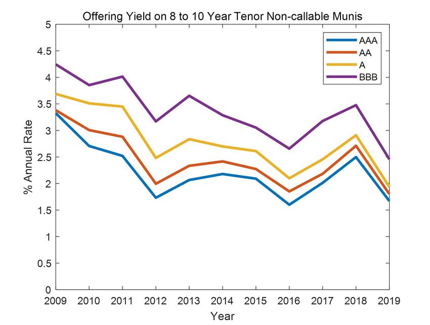
that, despite the much larger size of the corporate bond market (and that over half of
these bonds (and rising) also contain callable features), there is comparatively significantly
less value lost due to any delay in calling behavior over the same period and economy-
wide interest rate trends. This is consistent with a different behavioral disposition
regarding the timeliness of exercising the valuable option to call between corporate vs.
municipal issuers.4 One possible explanation for the differences between these two markets
is the sophistication of issuers and the underwriters that advise them on calling decisions;
we will test this hypothesis in Section IV.3.
 Over our data sample period of 2001-2018, several market conditions made it
optimal for municipal bonds to refinance. While issuance yields declined for all segments
of credit ratings in the municipal debt market, coupon rates of the existing callable debts
remained fixed around 5%, and there were significant tenors remaining after the call
options were unlocked. Figure 3 shows the coupon rate at issuance (Panel A) and the
remaining number of years to maturity at time of unlock (Panel B). We see that the mean
and median of coupon rates centers at 5% with most coupon rates falling between 4% and
6%. In addition, Panel B shows that the number of years remaining in unlocked bonds
ranged from 0 to 30, and most bonds have a significant amount of time left over so that
refinancing should be a key consideration.
 For refinancing to be optimal, bond yields must be low enough to offset future
coupon payments. In Figure 4, we show the offering yield of bonds offered between 2009
and 2018 over different credit rating buckets. While lower rated bonds naturally have
higher yields to compensate for their credit risk, we see that yields are low relative to the
average 5% coupon rates and have generally trended downwards across all bond ratings.
For example, while AAA bonds were issued with a yield of roughly 4.25% in 2009, they
were issued with a yield of 2.5% in 2019. This implies that, over time, there is a sizable
and rising premium for issuers redeeming and creating new issues.

IV.1.2 Comparison to Advance Refunding

 It is important to distinguish between refunding prior to the call unlock date (an
advance refunding) versus calling after the call option has unlocked (a current refunding).

4
 We detail our method of calculating value lost in Section IV.2.

 Calling All Issuers - 9

Delays to current refunding coexist with but are separate from advance refundings, which
are essentially synthetic early calls and are another key feature of the municipal market,
especially prior to 2018 when tax-exempt advance refundings was eliminated by The Tax
Cuts and Jobs Act of 2017.5 The set of advance refunded bonds and bonds with calling
delays are mutually exclusive. Since advance refunded bonds must call at the original
bond’s first call date, their calls are never delayed by definition. Therefore, all of our
results are empirically distinct (by construction) from advance refundings.

 That said, we were interested to explore the two phenomena more deeply to
understand any potential relationships in the data. Issuers that advance refund tend to
look different from those that call with delays. They are attentive to interest rates and
seek to benefit from reduced cash outflows (Ang et al. 2017). Conversely, as we find in
Section IV.3, issuers that delay calling appear to be less attentive to financial
opportunities and are more reliant on external financial agents to help them refund.
Consistent with this, we find that while a small number of issuers do both advance
refundings and delay current refundings, the overwhelming majority strongly prefer one
to the other - the correlation between percent of advance refundings and percent delays
within an issuer in our sample is -0.7. Finally, as we find in Tables 5 and 6, bonds which
are advance refunded have characteristics which are generally the opposite of bonds that
delay calling. For example, they tend to have larger coupons and have larger par amounts
than bonds which are called with a significant delay.

IV.1.3 Variation across States, Bond Types, and Credit Ratings

 In this section, we examine how calling delays vary within a number of observable
bond characteristics. In particular, we explore whether the delay in calling exists both
across and with three different dimensions: state of issue, bond type, and credit rating.
While there is significant variation across each of these categories, there is also significant
variation within each of them. So, across municipalities within the same state, within the

5
 Figure A1 shows the annual par amount of advance refunded bonds over time, and we see that there is a
steep drop in recent years beginning in 2018 due to the tax reform. While municipal bonds can still be
advance refunded into taxable bonds, these are less attractive to some investors, and thus, less attractive
to municipals as well.

 Calling All Issuers - 10

same bond type, and with the same credit rating, we see a large amount of variation in
calling behavior across municipalities.
 To begin the exploration, Table 2 summarizes the variation in delay to calling
across states, sorted by the size of each state’s municipal bonds outstanding. California,
New York, and Texas have the largest number of bonds outstanding with $344.6, $324.8,
and $232.0 billion outstanding, respectively. We see that there is significant variation in
the percent of bonds which delay by at least one year (Column 4) as well as the percent
that never call (Column 5). For example, while 35% of bonds are delayed in California,
only 12% are delayed in Connecticut. Figure 5 visually depicts the variation in the delay
to call across states. In Panel A, we show the percent of bonds that call with at least one-
year delay by state, and we see that there is substantial variation. While states like
California, Arkansas, and Mississippi delay more than 24% of their callable bonds, states
like Nevada and Utah delay less than 19% of their bonds. In Panel B, we show the percent
of bonds that never call at all, and we see a very similar pattern. States like Arkansas
never call at least 14% of their bonds, while states like Nevada never call less than 10%
of their bonds.
 Next, we find that there is variation in the decision to call across the funding
sources of municipal bonds. We see in Table 3 that 52% of bonds that are funded through
special taxes experienced redemption delays of one year or more. On the other hand, 18%
of General Obligation (GO) bonds, despite having the safest and lowest default probability,
experience redemption delays of one year or more. In fact, 11% of GO bonds with call
options unlocked between 2009 and 2018 never call.
 Finally, Table 4 summarizes the delay in calling by each bond’s credit rating at
the time when the call option unlocked.6 We see that despite having extremely high credit
quality, over 25% of bonds with a AAA rating delayed calling over our sample.
Furthermore, nearly 10% of AAA bonds never call. Likelihood of delay then broadly rises
as the credit quality declines. For example, over 31% of BBB rated bonds call with delays.

6
 We also break down the categories by whether the bond was downgraded prior to the unlock date. We
find that while downgraded bonds were more slightly likely to delay, downgrades do not explain a lot of
variation in calling delays. In general, for bonds with contemporaneous ratings of BBB or higher, the
likelihood of delay is similar for downgraded and non-downgraded bonds.

 Calling All Issuers - 11

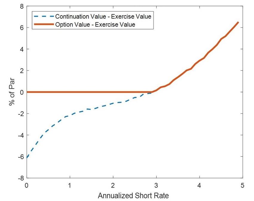
IV.2 Calculating Value Lost from Delay
IV.2.1 Understanding the Decision to Call
 In this section, we will consider the issuer’s decision to call a bond after its call
option has been unlocked. To begin, let’s consider a hypothetical 5% coupon bond with a
callable option. For simplicity, we assume that the callable option allows the issuer to call
the bond at par starting from a set date, which we will refer to as the unlock date. Panel
A of Figure 6 shows the expected cash flows if an issuer chooses to never exercise the call
option. In this case, the issuer receives the offering price at the beginning of the bond
issue and pays 5% coupon payments to the investors until the maturity date, when he
also returns the principal. On the contrary, if a call option is exercised, as shown in Panel
B of Figure 6, then the issuer pays off the principal before the maturity date. In this case,
the issuer can reissue the remaining cash flows at the current market price. If current
yields are lower than the coupon rate, then this bond can issue at a price higher than par
and capture a price premium. The exercise of the option is determined by how much of a
premium over par the subsequent coupon payments are currently valued at.
 The issuer essentially has an American call option on a non-callable but otherwise
identical bond, which pays coupons from the unlock date to the maturity date. At each
coupon payment date, there is an Exercise Value for exercising as well as a hypothetical
Continuation Value for not exercising the call and waiting till the next payment date
(assuming that the issuer only exercise at these intervals). If the continuation value is
greater than the exercise value, then the issuer should wait to redeem the bond. If the
exercise value is lower than the continuation value, then the issuer should exercise the
call option. If the issuer chooses to wait instead, then the differential between the Exercise
Value and the Continuation Value is lost.

IV.2.2 Valuing the Call Option
 We estimate the value of the call option using simple option value techniques. To
start, we chose a risk neutral dynamic for the market municipal rate, where we assume
that the market muni rate is a one factor random walk with a bound at zero. The yield

 Calling All Issuers - 12

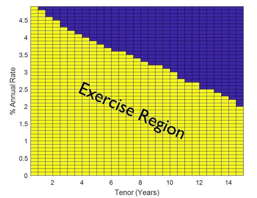
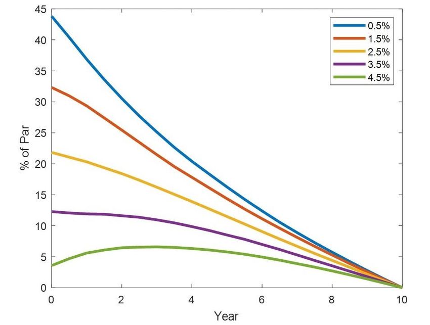
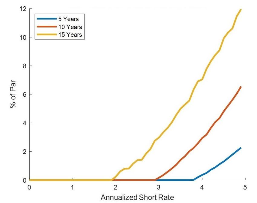
curve is flat, and we use 40 basis points as the volatility of the random walk.7 In Panel A
of Figure 7, we show the expected exercise values for different initial rates. The x-axis
shows the number of years from the unlock date, and in this example, we assume that
there are ten years left until the bond matures. Generally, for lower rates, the expected
exercise value is higher at the beginning of the bond’s life, because calling it captures more
value from coupon payments. Calling the bond at par on its maturity date at year ten
yields zero value.
 Next, we calculate the value lost when not exercising a call option. In Panel B of
Figure 7, for year zero, we plot the difference between the continuation value and the
exercise value in blue, and we plot the difference between option value and exercise value
in red. If current rates are high, then it is optimal to not exercise the option. In this case,
the value of the option and the continuation value are the same, and the issuer should
wait to call. On the other hand, when rates are low, then it is advantageous to immediately
exercise. Therefore, the option value is the same as the exercise value. When the exercise
value exceeds the continuation value, the value lost by not exercising is shown as the
difference between the red and the blue lines.
 Finally, we can calculate the optimal exercise bound for different rates and different
tenors. To do this, we follow the simulation methodology outlined in Longstaff and
Schwartz (2001). Figure 8 shows the time value of the call option for bonds with different
remaining maturities. For longer tenor bonds, it is only optimal to call when the rates are
sufficiently low. For shorter tenor bonds, the cost of losing a coupon payment exceeds the
option value of the bond going more into the money, and therefore, it is often more
optimal to exercise immediately even at higher rates. We can calculate the optimal
exercise regions for a range of different durations, current market issuance rates for similar
securities, and coupon rates. Figure 9 shows the two-dimensional optimal exercise region
for 5% semi-annual coupon bonds in yellow. In the next section, we generate this surface
for a cube of maturities, market rates, and coupon rates, and we match it to the empirical
data.

7
 This choice of volatility exceeds the physical standard deviation experienced by muni yields in the past
10 years. The semi-annual realized standard deviation of ten-year muni yields was about 30 basis per every
6 months. The options-implied volatility from the newly callable bonds is about 10 to 20 basis points.

 Calling All Issuers - 13

IV.2.3 Estimating Empirical Values
 In this section, we estimate the value lost from delays to exercise. We first take
the panel of callable bonds outstanding each year. Then, we group them into bins matched
by coupon rates (every 10 basis points), market yield (every 10 basis points), and the
number of coupon payment periods. 8 Using the aforementioned Merton model, we
estimate the optimal exercise value for each bin and the cost of delaying to exercise.
Finally, we sum the cost of delayed exercise for all callable bonds per year with investment
grade credit ratings from S&P.

 We find that the value lost from not exercising call options between 2001 and 2018
is large and economically meaningful. In Figure 2, we plot the dollar value estimated loss
from the delay to exercise. The annual value lost assuming a conservative 2% par value
issuance fee is shown in blue.9 We see that it begins at $0.24 billion dollars per year in
2001 and then rises to as high as $3.2 billion per year in 2012. To benchmark this figure,
we also plot a similar dollar value estimate of corporate bonds in orange over the identical
period, with similarly calibrated volatility and coupon rates. We estimate a significantly
lower magnitude for value lost in corporate bonds. These two estimates together indicate
that the variation in delays are specific to the municipal bond market.

IV.3 Explaining Variation in Delay

 Thus far, we have found that across the universe of municipal bonds, a sizable
percentage delay calling or do not call at all, which is generally suboptimal behavior given
the low interest rate environment over our sample period. Moreover, we observe
substantial variation in calling behavior across states, bond types, and credit ratings. In
this section, we explore whether there are factors systematically related to the bonds,
times, and agents involved in its issuance that can help understand the decisions to delay
calling behavior in more depth.

8
 For computational simplicity, we approximate all bonds as having semi-annual paying coupons.
9
 Based on issuance fees by state, our empirical data finds 1.2% fees on average, so this is a more conservative
estimate.

 Calling All Issuers - 14

To do this, we will use the following regression specification:

 , , = + + + , , + , , 

where , , is a dummy for delay of one year or more after bond has unlocked in
state s and year t ; and refer to state and year fixed effects respectively; and , , is
a vector of characteristics including: bond traits, proxies for issuer attention, underwriter
characteristics, and the persistence in relationship between a bond’s issuer and its
underwriter.

IV.3.1 Explaining Delays using Baseline Bond Characteristics
 In Table 5, we begin by examining how the variation in delay to call is related to
an initial set of observable traits of the municipal bond, within the state of issuance, bond
type, and credit rating. The dependent variable is a dummy for whether the bond, at the
time when its call option unlocks, delays the decision to call by at least one year.
Independent variables include: a dummy for whether the bond was downgraded prior to
its unlock date, remaining days-to-maturity after unlock, log size of issuance, coupon rate,
and offering yield. In these baseline regressions, based on our findings in Section IV.1, as
mentioned, we additionally control for state fixed effects, project type fixed effects, and
initial credit rating fixed effects, along with year of unlock fixed effects.

 From Table 5, we delays are positively related to both credit downgrades and
remaining months-to-maturity, while being negatively related to the size of the issuance,
coupon rates, and offering yield. Thinking through these initial relations, as there is more
of a premium to capture when coupon rates are higher than market rates, for instance, it
may not be a surprise that coupon rates are negatively and significantly related to delays
in Column 1. Next, from Column 2, as the coefficient is negative and significant, this is
consistent with the market offering a premium, or lower yields, to issuers who seem less
likely to call their bonds in a timely manner. However, as the R-squared is only 11%,
delays are likely not expected, nor completely priced in, at the time of issuance.

 When a bond is downgraded over its life, the issuer is suggested to have experienced
a credit-deterioration and is thus likely to face higher yields at refinancing. As shown in
Column 3, it is then not surprising that bonds with downgrades are 5.2% more likely to

 Calling All Issuers - 15

delay calling. As discussed in Section IV.2, as the remaining duration of the bond becomes
larger, there is more potential value in waiting to call. Consistent with this, in Column 4,
the coefficient on days-to-maturity is positive; however, it is not statistically significant
on its own at the 95% confidence interval (only in the multivariate full specification in
Column 6). Finally, in column 5, the size of the bond issuance is negatively and
significantly related to delays. This may be expected for a number of reasons – e.g., as
larger bond issues are likely more financially important and salient to issuers and
underwriters, one might expect them to be ceteris-paribus less likely to be neglected to be
called.

 In the last column of Table 6, we add all the baseline explanatory variables
simultaneously. We find that the coefficients generally remain the same, although the
coefficients on coupon and offering yield are halved in the joint specification. We interpret
this as due to the positive correlation between these two variables. In addition, days-to-
maturity becomes a significant predictor of delays in the multivariate specification. While
the fixed effects have an R-squared of 8% on their own, we see that adding these additional
factors significantly increases the r-squared to 14%.

 In Table 6, we then move on to comparing the traits of delayed calling behavior of
bonds with those of advance refunded bonds. Generally, we find that the characteristics
of advance refunded bonds are opposite to those of delayed bonds. From Columns 1-5, we
see that unlike delayed bonds, advance refunded bonds have larger coupons, have larger
offering yields, are less likely to be downgraded, have fewer days until maturity, and are
larger in size. These characteristics imply a bigger cash flow benefit to calling as soon as
possible, and they are consistent with the advance refundings being done by more
attentive municipals, which are cash constrained and looking to benefit from reduced net
cash outflows in the near future.

 Taken together, we find that several traits of municipal bond issuances, including
their coupon rates and offering sizes, are associated with their future calling delay. These
traits are quite different from advance refunded bonds. However, even after accounting
for these baseline traits, there is significant variation in the decision to call. In the next
section, we propose novel mechanisms that can explain calling delays: the roles of issuer

 Calling All Issuers - 16

workload and attentiveness, along with variation in the scope of external-agent debt
monitoring, and we will show that they both add significant richness and predictive power
in explaining the observed calling delay behavior of municipalities.

IV.4 The Roles of Workload, Attentiveness, and Debt Monitoring
IV.4.1 Issuer Workload and Attentiveness

IV.4.1.1 Fiscal Year-Ends
 Over our sample period, issuers on average call a bond seven months after the bond
becomes callable. This implies that the calling transaction is not immediate, but rather,
it may take some time to process. At a minimum, an evaluation of market rates and some
financial calculus are necessary in order to understand whether and when a bond should
be called. Moreover, as bonds are typically refunded through a new offering, it may take
time to decide how to structure the refunding bond. If an issuer is preoccupied with other
work or deadlines, they may be slower to call their bonds.
 For many local governments, the end of their state’s fiscal calendar is exactly this
type of time. Moreover, fiscal year-end is an especially busy time specifically for the
finance department, given their central role in the preparation, aggregation, processing,
and revision of annual municipal budgets across each division into the municipal-wide
fiscal budget. If this is the case, and it is not costless to temporarily modulate the size of
its staff month-by-month to accommodate both expected and unexpected work-flow
shocks, then there is a higher likelihood that the finance departments will face less time
(on average, all-else-equal) to attend to other activities. They may thus be less timely in
evaluating bond calls, and this may especially be true for smaller municipals with tighter
staffs.
 We test this hypothesis in Table 7. Namely, in Column 1, we regress the average
wait time between the unlock date and the day the bond is called on Fiscal calendar
dummies. Month before FY End, FY End, and Month after FY End are dummy variables
equal to one if the month that the bond’s call option unlocked was the month before its
state’s fiscal year end, the month of the fiscal year end, or the month after the fiscal year
end, respectively. We find that, controlling for other bond characteristics and fixed effects,

 Calling All Issuers - 17

bonds that are unlocked at fiscal year-end are on average delayed by an additional two
months (t=2.21). This suggests that, perhaps due to limited attention, the delay is not
immediately remedied in the month following the year end deadlines.
 In Columns 2 and 3 of Table 7, we test the hypothesis that smaller issuers,
presumably with less staff and financial expertise, are more adversely affected by fiscal
year end deadlines. In these specifications, we include a dummy for small issuer, which is
defined as one if it issued fewer than five bond issues over the sample period. We also
interact this dummy with year-end indicators in Column 3. First, from Column 2, small
issuers on average take significantly longer than others to call their bonds.
 Exploring more deeply in Column 3, we see two additional patterns. First, small
issuers experience roughly the same fiscal year end delays in the month of the fiscal year
end as larger issues (FY End coefficient + Small*FY End coefficient – while larger in
point estimate, is statistically equivalent). However, in addition to this, these small issuers
experience a strong and prolonged additional delay starting from the month before fiscal
year end (Coefficient on the interaction term of Small * Month before FY End of 0.449
(t=2.58)).
 Stepping back, the sum of the results in Columns 1-3 suggest that the especially
busy times of year for these issuers’ finance departments in particular – fiscal year-ends -,
coincide with delays to the exercise of call options, being especially true for smaller staffed-
issuing municipalities.
 Finally, in Column 4, we conduct a falsification test using revenue bonds. Revenue
bonds – unlike many other categories of municipal bonds – are not governed by the local
government but by the board of the project itself (e.g., hospital, road, nursing home
facility).
 As an example, consider a revenue bond from our sample in which the issuer was
the Port Authority of NY and NJ. It is the Port Authority Board of Commissioners listed
at the end of the bond issuance document, and deciding to call. Rather than following
New York’s fiscal year, which ends March 31, the Port Authority has a fiscal year that
ends on December 31, as reflected in its annual budget as well as the bond’s financial
operating filings. Thus, we would not expect this bond to follow New York State’s fiscal
cycle but rather that of its issuing entity.

 Calling All Issuers - 18

The results of this sample-wide falsification test are reported in Column 4 of Table
7. Reassuringly, we find no significant effect of local government fiscal calendars on calling
delays for revenue bonds.

IV.4.1.2 Workload Shocks due to Abnormal Unlocked Volume
 Depending on factors such as local budgets and bond ballot outcomes, municipal
borrowing may be lumpy and thus issuers may have years in which more bonds are
unlocked than normal. This leads to an even workload over time – often determined a
decade or more in the past when original issuance occurred. Nevertheless, these spikes in
workload could result in more calling delays, similar to the fiscal year-end result patterns
in Table 7. We explore this phenomenon in Table 8.
 In Table 8, for each bond at its call unlock date, we explore how a bond’s calling
delay is related to the abnormal workload its municipality is experiencing in the year of
its unlocking vis-à-vis the municipality’s normal level of refinancing. In Column 1, we
define issuer workload as the difference between the number of unlocked bonds and the
average number of unlocked bonds the issuer had to consider over the past ten years.
When this difference is larger, it implies a larger than usual workload. We find that
controlling for other bond characteristics, for each standard deviation increase in issuer
workload (3.1 bonds), the bond experiences roughly half a month additional delay time.
This effect is even stronger in Column 3 (roughly 30% larger), when we only consider
issuers who have had at least one callable bond to consider within the last ten years.
 In Columns 2 and 4, we then break down the proxy for issuer workload into its
individual components. We find that issuers who have had a larger numbers of bonds
unlock in recent times are significantly less likely to delay (Prev 10y Avg of Num Issues
Unlocked), consistent with larger municipals having more experienced and familiar
bandwidth for calling bonds. However, even controlling for this, we find that issuers who
have more bonds to consider calling in that given year (Num Issues Unlocked) are
significantly more likely to delay. Finally, in Column 4, we consider the subset of issuers
that had at least one bond unlock within the last ten years, and again we find that the
effect of the number of bonds unlocked in that given year is slightly stronger.
 In sum, the relationships from Tables 7 and 8 - attempting to proxy for issuer
workload and times of busy-ness using its work calendar and current workload – are
 Calling All Issuers - 19

consistent with both of these impacting the calling behavior that we find across
municipalities and over time. Overall, we find consistent evidence that when an issuer has
more constraints on its time, it is likely to result in, and elongate, a delay in its calling
decision.

IV.4.2 Debt Monitoring and the Role of Underwriters
 In the municipal finance market, underwriters play a critical role in the decision to
refund a municipal bond. They are not only responsible for issuing the bond, but they
also have incentives to monitor the bond over time and make sure it is not leaving money
on the table. When an underwriter helps a municipal call an old bond and refinance with
a new bond, they can earn a commission by underwriting the new issue. In this subsection,
we will consider how these key market monitors – and rich aspects of their relationships
to individual municipalities – are associated with calling delays.

 We begin by exploring first the basic industrial organization of municipal
underwriting. Empirically, underwriters vary substantially in terms of size as well as
geographic concentration. As a demonstration, in Figure 10, we plot the regional
dominance of three medium to large municipal underwriters in the United States:
Citigroup, Morgan Keegan, and Dougherty & Company LLC. Regional dominance is
defined as the ratio of the underwriter’s dollar amount underwritten in a state, divided
by the amount written by the state’s largest underwriter. For example, if Morgan Keegan
was the largest underwriter in Tennessee, it would have a regional dominance ratio of 1.
In contrast, if it did not underwrite at all in Tennessee, it would have a regional dominance
ratio of 0.

 As Figure 10 shows, some large firms like Citigroup (Panel A) write bonds all
around the country but are especially dominant in some regions, such as on the East and
West Coasts. In contrast, firms like Morgan Keegan and Dougherty are more narrowly
focused but very dominant in one geographic area. In particular, Morgan Keegan is
dominant in the South while Dougherty is heavily focused specifically in North and South
Dakota. Figure 10 highlights the geographical segmentation that characterizes municipal
finance markets. Moreover, it brings up the possibility that specialization (concentration)
in a specific region – such as that which Dougherty engages in - may offer a comparative

 Calling All Issuers - 20

advantage of specialized knowledge of local markets (to the extent it could be value-
relevant).

 To test whether underwriters’ geographic concentration affects calling delays, we
create a state-level measure of underwriter rank. In particular, for each state and year,
we sort the active underwriters by the total dollar amount underwritten in that state,
and we create a percentile measure of their size. For example, in 2009, if there were 100
active firms in Tennessee and Morgan Keegan underwrote more than all but 10 other
firms, then it would be in the 90th percentile and have a rank of 0.9.

 In Table 9, we explore the relationship between local underwriter concentration
and the delayed calling behavior of client municipalities. From Table 9, we find significant
evidence that bonds underwritten by locally dominant underwriters are less likely to delay
calling, even after controlling for underwriter fixed effects. First, in Column 1 of Table 9,
we regress a dummy for a bond with a calling delay of greater than one year on the
percentile rank of the bond’s lead underwriter. Consistent with the theory that locally
dominant underwriters pay more attention to their local bonds, we find that bonds are
significantly less likely to delay if they used an underwriter with a higher rank. The top
underwriter in the state (with a rank of 1) is associated with a bond that is 8 percentage
points (t=9.33) less likely to delay compared to a bond associated with the smallest
underwriter (with a rank of 0).

 Interestingly, it is not the overall national size of the underwriter but rather the
relative size of the underwriter in the local market that matters. To test this, in Column
2 of Table 9, we add underwriter fixed effects in addition to the underwriter rank, and we
still find a negative, significant coefficient on underwriter rank. This suggests that even
within a given underwriter, the local specialization of that underwriter in the given market
matters. For example, even if two bonds used the same underwriter, such as Citigroup,
the bond which is located in a state that Citigroup is the top underwriter (has a rank of
1) would be five percentage points (t=3.47) less likely to delay than a bond located in a
state that Citigroup is bottom (has a rank of 0).

 In addition to the local size of the underwriter, we find that generally more
competitive markets are associated with fewer calling delays. In Table 9, Column 3, we

 Calling All Issuers - 21

include the number of active underwriters in the state as an additional covariate. We find
that bonds whose call options are unlocked in markets with more underwriters are
significantly less likely to delay calling. Even controlling for state fixed effects, we find
that each additional underwriter is associated with a 1.2 percentage point (t=2.23) smaller
probability of calling delay. Finally, in Column 4, we add in the rank of the underwriter
along with the number of active underwriters, and we find that both variables are
negatively and significantly related to calling delays.

IV.4.3 Persistence in Underwriter and Issuer Relationships
 While some underwriters are less efficient at monitoring than others, ultimately,
bond issuers can choose their agents and always have the option of switching underwriters.
Relatedly, underwriters themselves are open to actively approach municipalities that use
their competitor underwriters to generate new business. The decision to switch may be
particularly poignant if not switching can cost them millions in borrowing costs. In this
section, we explore the nature of municipality-underwriter relationships.

 The first strong empirical regularity we find is that most municipal issuers are slow
to switch lead underwriters, and these persistent, sticky relationships can help explain
part of the variation in calling delays. This may be because issuers prefer the underwriter
for other reasons other than refinancing efficiency (e.g., some other bundled good or service
– either observable or unobservable - that the underwriter provides), or because they are
not aware that there are better underwriters in the market. In addition, small or
infrequent issuers may not be able to offer enough business to attract the largest
underwriters.

 Table 10 provides summary statistics for the market, and initial evidence of this.
In particular, from Table 10, on average each municipal issues 87% of all of its bonds
using the same lead underwriter. To control for the fact that some issuers may only sell
a few bonds or sell many bonds at once as part of the same series, we restrict our sample
to issuers who have issued at least 20 (Row 2), 40 (Row 3), or 60 bonds (Row 4). We see
that a pattern of persistent relationships holds even after restricting our sample to issuers
with at least 60 bonds: on average, they underwrite over than half of their bonds using

 Calling All Issuers - 22

the same underwriter. Finally, we show that issuers who use Bear Stearns (Row 5) and
Lehman (Row 6) have very persistent relationships. We will later use this observation to
examine shocks to the underwriter-issuer relationship.
 Next, we create a measure that captures the persistence of the issuer’s relationship
with its underwriter, and we show that persistence of the underwriter relationship is
associated with more delays. For each issuer and underwriter pair, our measure is
calculated as the dollar-weighted percentage of all bonds that are underwritten by the
same lead underwriter. To ensure that this relationship is relevant at the time of the
refinancing decision (i.e., no look-ahead bias), we examine data solely looking backward
at each point in time from the last ten years prior to the bond’s call unlock date. For
example, suppose a bond’s call option unlocked in 2001, and the given municipality
underwrote 10 billion dollars of bonds with Lehman from 1991 to 2000. If the bond’s issuer
issued 40 billion dollars of bonds total over 1991 to 2000, then we would measure its
persistence with Lehman as 10/40 or 0.25.
 We find that bonds that use a persistent underwriter are significantly more likely
to delay calling, holding as else equal. In Figure 11, for instance, we show a scatterplot of
our underwriter persistence measure versus a dummy equal to one if the bond delayed
calling by at least one year. We see that there is a strong and positive linear relationship.
Next, we test this relationship more formally in Table 11. From Column 1 of Table 11,
controlling for state, year, credit rating, and capital purpose fixed effects, we find that
when a bond comes from an issuer that relies heavily on its lead underwriter (persistence
of one), it is eight percentage points more likely to delay calling than if it used an
underwriter that it no longer uses (persistence of zero). In column 2, we further show that
underwriter persistence adds additional explanatory power even controlling for the other
bond characteristics from Table 5.
 Lastly, in Column 3 of Table 11 we explore to what extent local expertise -
positively associated with monitoring in Table 10 – helped to mitigate the impact of sticky
relationships. This is to say, if the long-standing, sticky relationship were with a locally
specialized underwriter, would that attenuate this negative association of monitoring.
From Column 3 of Table 11, that is exactly what appears to happen. As in Table 10, have
a locally specialized underwriter (all else equal) reduces the incidence of call delays on a
municipal’s bonds. Moreover, the sticky relationship that results in significantly more
 Calling All Issuers - 23