Munich, 4-5 July 2019 Rational Inattention and Migration Decisions - Simone Bertoli, Jesús Fernández-Huertas Moraga, and Lucas Guichard - ifo Institut
←
→
Page content transcription
If your browser does not render page correctly, please read the page content below
Munich, 4–5 July 2019

Rational Inattention and Migration Decisions
Simone Bertoli, Jesús Fernández-Huertas Moraga, and Lucas Guichard
Rational inattention and migration decisions∗
Simone Bertolia , Jesús Fernández-Huertas Moragab , and Lucas Guicharda,c
                        a
                            Université Clermont Auvergne, CNRS, IRD, CERDI†
                                   b Universidad   Carlos III de Madrid‡
                                                    c IAB§

                                                 Abstract

       We analyze the implications of introducing a cost related to acquiring information on
       the attractiveness of the alternative destinations in the decision problem that migrants
       face. This extension of the canonical model entails that individuals with stronger priors
       about the identity of their utility-maximizing alternative rationally gather less informa-
       tion. The theoretical model gives us an analytical expression for the expected value of
       information that can be computed from past migration data. The econometric analysis
       reveals that migration flows originating from countries characterized by stronger priors
       are significantly less responsive to variations in economic conditions at destination.

Keywords: international migration; information; gravity equation.
JEL codes: F22; D81; D83.

   ∗
      The Authors are grateful to Rabah Arezki, Erhan Artuç, Vianney Dequiedt, Lionel Fontagné, Joël
Machado, Thierry Mayer, David McKenzie, Çağlar Özden, Panu Poutvaara, Ariell Reshef, Victor Stephane,
Jérôme Valette, and to the participants at seminars at CERDI, the World Bank, Université Paris 1 Panthéon-
Sorbonne, IAB and to the IZA-CREA Workshop on “Gravity equations in International Economics: When
Trade Meets Migration” (University of Luxembourg) for their comments; the Authors are also grateful to
Sergio Correia, Paulo Guimarães and Thomas Zylkin for sharing the Stata command ppmlhdfe with us
before it became publicly available, and to Olivier Santoni fo providing valuable research assistance; Si-
mone Bertoli acknowledges the support received from the Agence Nationale de la Recherche of the French
government through the program “Investissements d’avenir ” (ANR-10-LABX-14-01), and from the Institut
Universitaire de France; Jesús Fernández-Huertas Moraga acknowledges the financial support from the Min-
isterio de Economı́a, Industria y Competitividad (Spain), grants ECO2016-76402-R and MDM 2014-0431,
and from the Comunidad de Madrid, MadEco-CM (S2015/HUM-3444); the usual disclaimers apply.
    †
      CERDI, Avenue Léon-Blum, 26, F-63000, Clermont-Ferrand; email: simone.bertoli@uca.fr.
    ‡
      Madrid, 126, E-28903, Getafe (Madrid); email: jesferna@eco.uc3m.es.
    §
      Regensburger Strasse, 104, D-90478 Nuremberg; email: lucas.guichard2@iab.de.

                                                      1
“Before making a choice, one may have an opportunity to study the actions and their payoffs; however, in
most cases it is too costly to investigate to the point where the payoffs are known with certainty. As a
result, some uncertainty about the payoffs remains when one chooses among the actions even if complete
information was available in principle.”
(Matějka and McKay, 2015, p. 272)
1 Introduction
The canonical micro-foundations of a gravity equation for international migration draw on
discrete choice models à la McFadden, which were initially conceived to describe consumption
choices, that assume that the decision maker costlessly observes the realizations of the payoff
associated to each alternative in the choice set before selecting her preferred option. This
analytical choice is not immaterial, as “[c]onsumers are continually making choices among
products, the consequences of which they are dimly aware” (Nelson, 1970, p. 311), and
this just partial awareness, a fortiori, applies to individuals that have to decide where to
migrate. The uncertainty surrounding the utility associated to the various countries of
destination might not be entirely resolved when a migrant has to come up with a solution
to the location-decision problem that she faces,1 and the size of the remaining uncertainty
could be endogenously determined by migrants’ choices to refine their knowledge about the
actual attractiveness of the various destinations, as the initial quote by Matějka and McKay
(2015) suggests.2 The literature on rational inattention (Sims, 1998, 2003), which has been
recently applied to discrete choice situations (Matějka and McKay, 2015; Caplin et al., 2019),
provides us with a framework to think about how costs associated to information acquisition
and processing would influence the specification of the migration gravity equation that is
brought to the data.
Can we sharpen our understanding of the determinants of international migration flows if
we take into account the uncertainty that migrants face, and the actions that they can take
to narrow it down? We propose an extension of the standard additive random utility max-
imization model used in the migration literature featuring a rationally inattentive behavior
1
See McKenzie et al. (2013) for empirical evidence on the inaccuracy of the expectations held by potential
migrants on their earnings in a foreign labor market.
2
In his seminal contribution, Simon (1959) observed that information “should be gathered up to the
point where the incremental cost of additional information is equal to the incremental profit that can be
earned from having it.” (pp. 269–70).
2of the migrants. The main prediction of this model is that the responsiveness of bilateral
migration flows with respect to variations in the attractiveness of alternative destinations in-
creases when migrants have stronger incentives to acquire information before deciding where
to move. These incentives are inversely related to the strength of the migrants’ prior beliefs
about the identity of their preferred destination, and we propose a way to measure this
strength using data on the distribution of past bilateral migration flows. The estimation of
a gravity equation reveals that variations in economic conditions in a given destination in-
fluence more incoming migration flows from origins where migrants (rationally) invest more
in information acquisition.
The contribution of our paper is threefold. First, we extend the canonical microfounda-
tions of the gravity equation in the international migration literature to allow for a costly
acquisition of information about the attractiveness of the various destination countries, draw-
ing on the recent contributions by Matějka and McKay (2015) and Caplin et al. (2019). We
derive an analytical expression for the value of observing the actual individual-specific utility
in each alternative in the choice set, which is inversely related to the strength of the priors
held by the migrants. Second, we propose an empirical counterpart of the theoretical expres-
sion for the value of information, which is given by (minus) the logarithm of the origin-specific
share of migrants in the main destination over a period ranging from 5 to 20 years before
the one over which we measure migration flows. We show that this variable significantly
mediates the responsiveness of observed bilateral migration flows with respect to variations
in economic conditions at destination, uncovering a relevant dimension of heterogeneity that
had remained so far unnoticed. Third, we provide evidence of the empirical relevance of
rational inattention in discrete choice situations, complementing a strand of literature that
it is still mostly theoretical.3 Migrants appear to be rationally inattentive even though the
stakes related to their location decisions are certainly very high (see, for instance, McKenzie
et al., 2010 and Clemens et al., forthcoming).
We draw on data on bilateral migration flows between 1960 and 2015 from Abel (2018)
to build an origin-specific time-varying measure of the value of information for international
migrants, whose functional form comes directly from our theoretical model. We estimate
a gravity equation where the deterministic component of destination-specific utility is aug-
mented with an interaction between income per capita and the empirical counterpart of our
3
“The model of [rational inattention] is well suited for a boom in empirical work, which has not yet
occurred.” (Maćkowiak et al., 2018, p. 27).
3measure of the value of information. The results are in line with the theoretical model: a one
standard deviation increase in our proxy for the value of information determines an increase
in the estimated elasticity between 0.063 and 0.083. Our estimates entail that the elasticity
of the bilateral migration rate with respect to income per capita for China is 0.160-0.216
higher than the corresponding elasticity for Mexico, which represents a paradigmatic case of
migration flows concentrated in just one single destination, the United States. The econo-
metric evidence that we provide is fully robust when we allow for additional heterogeneity
of this elasticity at the origin or at the dyadic-level.
Our paper is related to and contributes to three different strands of literature: (i ) ra-
tional inattention in discrete choice models, (ii ) micro-foundations of the migration gravity
equations, and (iii ) migration models with residual uncertainty.
As far as rational inattention in discrete choice models is concerned, the closest reference
to our theoretical model is Matějka and McKay (2015). They consider a discrete choice
model where the decision maker chooses the precision of the signals that she receives about
the payoffs of the various alternative in the choice set, with the cost of observing the signal
being proportional to the ensuing reduction in the Shannon or differential entropy associated
to the distribution of payoffs (Shannon, 1948). Matějka and McKay (2015) demonstrate that
choice probabilities depend on the actual (but possibly unobserved) values of the payoffs,
and on the prior beliefs that individuals have about the attractiveness of each alternative in
the choice set, which shape the chosen information-processing strategy. The decision maker
could rationally decide to completely disregard some of the alternatives in the choice set
(Caplin et al., 2019), thus choosing with a positive probability in any state of the world
only a subset of options belonging to the so-called consideration set, something that would
never occur if information was costlessly available. Our reliance on the distribution of past
migration flows across destinations to measure the value of information acquisition is closely
related to the use of past market shares in Caplin et al. (2016). Dasgupta and Mondria
(2018) have drawn on Matějka and McKay (2015) to extend the Ricardian model of trade
by Eaton and Kortum (2002), allowing for a costly acquisition of information on the prices
of a good in different countries. The main prediction of their model refers to the non-
monotonicity of the relationship between the number of distinct countries from which the
same good is imported and the unitary cost of information, with the data being consistent
with the predicted hump-shaped relationship between the two variables.
4With respect to micro-foundations of the migration gravity equations, our paper is related
to papers that have derived a specification of the gravity equation under more general distri-
butional assumptions on the stochastic component of utility, notably Bertoli and Fernández-
Huertas Moraga (2013) and Ortega and Peri (2013), as these more general specifications
have allowed uncovering additional determinants of bilateral migration flows. Batista and
McKenzie (2018) have tested in the lab these micro-foundations, notably allowing players to
pay a cost to reduce the uncertainty about the payoffs associated to the various destinations.
Fosgerau et al. (2018) have recently drawn a bridge between the first two strands of litera-
ture that our paper is related to. Specifically, they demonstrate that choice probabilities in
Matějka and McKay (2015) follow a modified logit formula because of the reliance of Shannon
entropy to measure the cost of information acquisition.4 Relying on a generalized entropy
function, which allows for spillovers in information acquisition across alternatives, results
in choice probabilities that can be derived from any additive random utility maximization
model.
Finally, our paper is related to models of migration with unresolved uncertainty that
arises either because utility at destination is not remotely observable (Bertoli, 2010), or
because of the repeated nature of the location-decision problem that migrants face (Kennan
and Walker, 2011; Bertoli et al., 2016; Artuç and Özden, 2018), with location choices that
can be revised as individuals draw new realizations of the stochastic components of utility
in each period.5
The rest of the paper is structured as follows: Section 2 combines the canonical additive
random utility maximization model with rational inattention arising from a costly acquisition
of information about the attractiveness of the various destination countries; Section 3 briefly
presents the main data sources, it describes how we bring the testable implication of the
theoretical model to the data, and it presents basic descriptive statistics. Section 4 presents
the results of the estimation of the migration gravity equation that allows for rationally
inattentive location choices, and Section 5 concludes.
4
See also Caplin et al. (2017) for a characterization and a generalization of Shannon entropy in models
of rational inattention.
5
Steiner et al. (2017) include rational inattention in a dynamic discrete choice model.
52 Theoretical model
Let uijk denote the utility that migrant i from the origin j derives if she opts for country
k ∈ A, where A represents her choice set, with #A = N , which does not include country
j itself, so that we focus here on the choice of the destination conditional upon migrating.
Assume that uijk is additive in a deterministic component of utility, vijk , and in a stochastic
component, ijk :6
uijk ≡ vijk + ijk (1)
Let vij = (vij1 , vij2 , ..., vijN )0 , ij = (ij1 , ij2 , ..., ijN )0 , and eij = (eij1 , eij2 , ..., eijN )0 represent
three N × 1 column vectors stacking respectively the deterministic component of utility, the
stochastic component of utility and its realizations across all alternatives in the choice set A.
The standard micro-foundations of this location-decision problem are based on distributional
assumptions à la McFadden (1974), with:
P
F (ij ) = e− k∈A t(ijk )
(2)
where t(ijk ) = e−(ijk +γ) and γ ≈ 0.5772 is Euler’s constant,7 as an identically and indepen-
dently distributed EVT-1 stochastic component of utility allows to derive a specification a
for gravity equation that can be easily estimated with aggregate data.8
The stochastic component of location-specific utility in (1) can reflect both individual
heterogeneity in preferences and aggregate uncertainty about the attractiveness of alternative
k ∈ A, while maintaining the distributional assumptions described in (2). Specifically, we
could define:
ijk ≡ Cjk (αk ) + αk ηijk , (3)
with αk ∈ (0, 1], ηijk following an EVT-1 distribution, and Cjk (αk ) being the (unique) ran-
dom variable that ensures that ijk also follows an EVT-1 distribution (Cardell, 1997). If
αk = 1, then Cjk is equal to an arbitrary constant, and it is not stochastic, so that (3) also
6
The cost of moving from the origin j to the destination k is included into the dyadic deterministic
component of utility.
7
The inclusion of γ in the expression for t(ijk ) ensures that the expected value of the stochastic com-
ponent of utility ijk is equal to 0.
8
This occurs because the dependence of bilateral migration flows on the attractiveness of alternative
destinations in the choice set can be controlled through a suitable normalization of the dependent variable,
as it occurs in the Ricardian model of trade by Eaton and Kortum (2002), while the same would not occur
with a normally distributed stochastic component, as in Roy (1951) or Borjas (1987).
6nests the case in which the stochastic component of utility only reflects unobserved individual
heterogeneity. Cjk (αk ), which does not vary across individuals, captures the aggregate un-
certainty for migrants from j about the attractiveness of alternative k ∈ A, and the relative
importance of individual heterogeneity and aggregate uncertainty, described by αk , could be
destination-specific. Assuming that Cjk (αk ) and ηijk are independently distributed across al-
ternatives in the choice set ensures that ijk is consistent with the distributional assumptions
laid out in (2). The inclusion of Cjk (αk ) in (3) entails that, as in Matějka and McKay (2015),
the migrant faces an uncertainty about the state of nature that influences location-specific
utility, while the individual-specific stochastic component ηijk might be perfectly known to
her. This entails that our framework is fully consistent with a classical interpretation of
the stochastic component of utility, which reflects the imperfect knowledge of the modeler.9
Thus, we do not need to assume here, as in Caplin et al. (2016), that the decision maker is
uncertain about her own preferences over the various alternatives in the choice set.
2.1 Migrants’ information set
We analyze this location-decision problem under two alternative assumptions on the infor-
mation set to which migrants have access before choosing their preferred destination: the
canonical full information case, where migrants observe both vij and eij ,10 and a partial
information case, where migrants only observe vij . This second more limited information set
is meant to represent a (limit) case of the constraints on the capacity to process information
that could characterize migrants’ decisions, and it will help us to understand what shapes
the incentives to acquire and process information.
2.1.1 Full information
Let us define the real-valued function V (vij + eij ) that returns the utility associated to
the utility-maximizing alternative in A. Formally, V : RN → R, with V (vij + eij ) ≡
9
“The econometricians’ approach is conceptually very different [...] both the decision rule and the utility
functions of the individual are deterministic. The uncertainty is due to the lack of information available to
the modeler.” (Anderson et al., 1992, pp. 31–33, emphasis in the text).
10
Borjas (1987) assumes that migration decisions are based on a comparison of “potential incomes” at
origin and at destination (p. 532), with the latter being remotely observable, i.e., known before migrating, in
line with the analysis by Roy (1951) on the occupational choice between hunting and fishing that explicitly
assumes that “[e]very man, too, has a fairly good idea of what his annual output is likely to be in both
occupations” (p. 137).
7maxk∈A (vijk + eijk ). Similarly, we can define a : RN → A as the alternative in the choice set
A such that (vija + eija ) = maxk∈A (vijk + eijk ). Under the distributional assumptions that
we introduced above, the ex ante probability that alternative k is the utility-maximizing
alternative for individual i is given by (McFadden, 1974, 1978):11
evijk
pijk = P vijl
(4)
l∈A e
Notice that the decision rule of individual i is not probabilistic, as the vector eij is observed
before deciding where to migrate; by the law of large numbers, pijk coincides with the
share of i-type individuals from the origin j that find it optimal to migrate to k. The
expected utility from the choice situation is given by the integral, over the distribution of
ij , of V (vij + ij ), the utility associated to the utility-maximizing alternative. Under the
distributional assumptions introduced above, we have that (Ben-Akiwa and Lerman, 1979;
Small and Rosen, 1981): !
X
Eij [V (vij + ij )] = ln evijl (5)
l∈A
2.1.2 Limited information
What if the decision to migrate has to be taken observing just vij ? In this case, migrant i
should opt for the alternative characterized by the highest deterministic component of utility.
We can define the real-valued function W (vij ) that returns the highest deterministic com-
ponent of utility in the choice set A. Formally, W : RN → R, with W (vij ) ≡ maxk∈A vijk .
Similarly, we can define c : RN → A as the alternative in the choice set A such that
vijc = maxk∈A vijk . The expected utility from opting for alternative c ∈ A is simply given
by: Z +∞
Eij [W (vij )] = uijc dijc = vijc (6)
−∞
2.2 Rational inattention
Let us consider the case in which the realizations of the stochastic component of utility can
be observed by individual i, but this observation comes at a cost. In line with the literature
on rational inattention (Matějka and McKay, 2015), we assume that the cost of acquiring
11
Luce and Suppes (1965, p. 338) credit unpublished work by Holman and Marley for this result.
8information on the actual values of location-specific utility is proportional to the entropy
of the multivariate distribution of utility, i.e., the vector vij + ij . We derive next the cost
of a (discrete) switch from the partial to the full information case described above, and we
also derive the expected value of acquiring (full) information on the values of the stochastic
components of utility.
2.2.1 The cost of acquiring information
Let B denote the belief of migrant i about the distribution of the stochastic component of
utility, and let us assume that B coincides with the actual distribution described in (2). The
differential entropy H(B) associated to this distribution is given by:
Z
H(B) ≡ − f (ij ) ln f (ij ) dij (7)
ij
where f (ij ) is the probability density function corresponding to the cumulative density
function in (2). The joint entropy of N independent distributions is given by the sum of
their individual entropies (see, for instance, Cover and Thomas, 1991), while the assumption
that the distributions are identical entails that the joint entropy in (8) is given by H(B) =
P
k∈A H(ijk ); the entropy H(ijk ) of a univariate distribution is equal to:
Z +∞
H(ijk ) = − f (ijk ) ln f (ijk ) dijk (8)
−∞
With some simple algebraic manipulations,12 we have that:
Z +∞
H(ijk ) = [t(ijk ) + (ijk + γ)]f (ijk ) dijk
−∞
Z +∞
= t(ijk )f (ijk ) dijk + γ
−∞
Z +∞ (9)
+∞
= [t(ijk )F (ijk )]−∞ + t(ijk )F (ijk ) dijk + γ
−∞
Z +∞
+∞
= [f (ijk )]−∞ + f (ijk ) dijk + γ = 1 + γ
−∞
12
We use the fact that f (ijk ) = t(ijk )F (ijk ), and we rely on integration by parts to integrate
t(ijk )f (ijk ), with the indefinite integral of t(ijk ) being −t(ijk ).
9Letting λk ∈ R+ , with k ∈ A, denote the destination-specific parameter that converts entropy
into the metric of utility, the cost c(λA ) of switching from partial to full information is given
by:
c(λA ) = λA (1 + γ) (10)
P
where λA ≡ k∈A λk .
2.2.2 The value of acquiring full information
The value wij of observing the realization of the stochastic component of utility is given by
the difference between the value of the choice situation under full and partial information,
i.e., Eij [V (vij + eij )] − Eij [W (vij )]. From (5) and (6), we have that wij is equal to:
!
X
wij ≡ Eij [V (vij + eij )] − Eij [W (vij )] = ln evijk − vijc = − ln[pc (vij )] (11)
k∈A
where pc (vij ) ∈ [1/N, 1] is the probability that the destination with the highest deterministic
component of utility has also the highest utility, i.e., pc (vij ) = Prob [c(vij ) = a(vij + eij )].
Figure 1: The value of full information wij
wij
ln(N )
− ln(p)
c(λA )
0
1/N ()p() e−c(λA ) 1 pc (vij )
The value of full information is a monotonically decreasing function of this probability, as
shown in Figure 1. Intuitively, the acquisition of information increases the expected utility
derived from the choice situation only if it leads to a change in the alternative in the choice
10set that is selected by the migrant. The higher is pc (vij ), the lower are the chances that a
(costly) acquisition of information would induce the migrant to modify the location choice
based on her priors. We can refer to pc (vij ) as the strength of migrant’s priors, based on
exclusively vij , concerning the identity of the utility-maximizing destination in the choice
set.
2.3 Strength of the priors and return from acquiring information
The value of acquiring information is negatively related to the strength of the priors held by
migrant i, while the cost in terms of utility of such an investment is independent from the
strength of the priors. Thus, the expected return πij (vij , λA ) from acquiring information,
given by the difference between (11) and (10), is equal to:
πij (vij , λA ) = wij − c(λA ) = − ln[pc (vij )] − λA (1 + γ) (12)
When information acquisition is costly, migrants with stronger priors will tend to be ratio-
nally inattentive, as the acquisition of information about the actual attractiveness of the
various destinations in the choice set is unlikely to induce them to modify their destination
choices, and it is thus associated with a lower value of πij (vij , λA ). Furthermore, (12) implic-
itly defines a threshold value of pc (vij ), depicted in Figure 1, such that migrants will certainly
not find profitable to acquire full information when pc (vij ) > p(λA ) ≡ e−c(λA ) even if this
was potentially available, as the initial quote from Matějka and McKay (2015) suggests.13
Migrants are not constrained to select one of the two polar cases that we have analyzed, as
they could opt for observing Bayes-consistent signals about location-specific utility (Matějka
and McKay, 2015), possibly gathering information just on a subset of the choice set A,
rationally disregarding alternatives that are, a priori, extremely unlikely to be the utility-
maximizing option (Caplin et al., 2019). Rational inattention results in choice probabilities
that have a structure that resembles a canonical conditional logit but that depend both on
the actual (but possibly unobserved) attractiveness of each alternative, and on the prior
beliefs held by the decision maker.14
13
Notice that pc (vij ) > p(λA ) represents a sufficient but not a necessary condition for migrants rationally
deciding not to acquire full information on the attractiveness of each alternative in the choice set A.
14
Appendix A.1 reports the choice probabilities that solve the location-decision problem with costly
information acquisition.
11This gives us a clear testable implication: if the stochastic component of location-specific
utility also includes an aggregate component, as in (3), and the actual investment in infor-
mation acquisition is proportional to the return from acquiring full information in (12),15
then migration flows should be less responsive to variations in the attractiveness of the des-
tination countries when migrants have stronger priors. Rationally inattentive migrants with
strong priors (optimally) decide to gather less information about the attractiveness of the
various destinations, and hence their location choices are less sensitive to variations in, say,
economic conditions than we would expect when full information can be costlessly acquired.
The theoretical model does not just give us a qualitative prediction, but also very specific
guidelines with respect to the functional form, described in (12), of the relationship between
the return from acquiring information and the strength of migrants’ priors.
3 From the theory to the data
We describe here the source of our panel data on bilateral international migration flows, and
how we build from these data the empirical counterpart of the theoretical definition of the
value of information. We also present basic descriptive statistics, focusing in particular on
our variable of interest.
3.1 Data on bilateral migration flows
Our main data source is represented by Abel (2018), which provides data on the bilateral
migration flows mjkt ≥ 0 between the origin j and the destination k across 203 countries for
five-year periods, starting in t, between 1960 and 2015. Abel (2018) extends the methodology
presented by Abel and Sander (2014) for inferring gender-specific bilateral migration flows
from information on the stock of individuals (by country of birth) residing in each country
obtained from population censuses. More precisely, Abel (2018) recovers the minimal amount
of bilateral flows that are required in order to match the observed evolution of stock data,
which are adjusted for demographic events. The stock data are taken from Özden et al. (2011)
between 1960 and 2000, and from United Nations Population Division (2015a) for later years,
15
The Appendix A.2 shows that, in a simplified version of the model that is analytically tractable, the
actual investment in information acquisition is bounded from above by a term that is proportional to the
return from acquiring full information.
12and are combined with demographic information from United Nations Population Division
(2015b) to obtain the estimates on flows. To our knowledge, the dataset generated by Abel
(2018) is the most comprehensive in terms of both time and geographical coverage produced
to date on international migration flows.16 As discussed below, these two aspects are critical
to generate from the data the empirical counterpart of the value of information described in
our theoretical model. The sample over which we conduct our econometric analysis includes
the entire set of countries covered by Abel (2018): for the period between 1980 and 2015,
we have 263,008 observations on bilateral migration flows over seven consecutive five-year
periods.17,18 The average value of mjkt stands at 957.4, with a standard deviation of 15,472.4
and a share of zero flows equal to 61.2 percent.
3.2 Measurement of the value of information
The theoretical model predicts that the return from information acquisition in (12) depends
on the strength of migrants’ priors concerning the (time-varying) identity of the utility-
maximizing destination, and on the cost of acquiring information. This requires building
from the data a suitable empirical counterpart of the value of information, and dealing in
the econometric analysis with the challenges related to the unobservability of the cost of
information. Our assumption is that current migrants from j have observed the destination
choices made in the past by individuals leaving from j itself, and their distribution across
destinations has shaped the strength of their priors. The location-decision problem presented
in Section 2 is static, and it allows for individual heterogeneity; the availability of longitudinal
data on bilateral migration flows that are not disaggregated (except for the gender dimension)
entails here that we have to assume that choice probabilities in (4) are constant across
individuals for a given origin but possibly time-varying. Thus, we proxy the time-varying
strength of the priors for the origin country j in year t with the share of migration flows
directed from j to the main foreign destination in a period up to t. More precisely, we rely
16
Our empirical evidence is robust to using only the bilateral flow data in Abel (2018) that are based
solely on migrant stocks from Özden et al. (2011), thus avoiding possible inconsistencies at the junction
between the two underlying data sources, and to defining bilateral migration flows as the variations in the
stock of j-born individuals residing in destination k derived from Özden et al. (2011).
17
Migration flows before 1980 are used to measure the empirical counterpart of the value of information,
as discussed in Section 3.2 below.
18
This is below 203 × 202 × 7 = 287, 042 as we have missing information of GDP per capita at destination
for some destination-year pairs; more precisely, we lose completely 14 destination countries, which represent
less than 0.9 percent of total migration flows in Abel (2018).
13on p(r)jt , defined as follows:19
( Pt )
mjkt
p(r)jt ≡ max Pt t−r
P , r = {5, 10, 15, 20} (13)
l∈A mjlt
k
t−r
It is interesting to note that 107 different countries represent the main destination, and
hence determine the value of information, for at least one of the 1,349 origin-year pairs in
our estimation sample; intuitively, the United States are the most typical main destination
accumulating most of the flows for a particular origin, but this happens only in 20.7 percent
of the cases; the second most typical main destination is Russia, for 7.6 percent of all origin-
year pairs, and five Sub-Saharan African countries (namely, South Africa, Ethiopia, Nigeria,
the Democratic Republic of the Congo, and Ivory Coast) appear among the 20 countries
that most frequently play the role of main destination. We then measure, following (11), the
value of information for the origin j at time t as:
w(r)jt = − ln[p(r)jt ] (14)
To give concrete examples, we have that 97.0 percent of flows from Mexico between 1990
and 1995 were directed to the United States, so that w(5)MEX1995 = − ln(0.970) = 0.031.
Over the same period, 25.4 percent of migration flows from China were directed to the main
destination (United States), and this entails that w(5)CHN1995 = − ln(0.254) = 1.371. Thus,
the empirical counterpart of the value of information in (14) entails that Chinese migrants
valued information more than Mexican migrants in the five-year period starting in 1995, as
the latter group of migrants held substantially stronger priors with respect to the identity
of the utility-maximizing destination.
19
Notice that p(r)jt in (13) is defined provided that the total flow originating from j between year t − r
and t is positive; this is always the case except for 31 origin-year pairs when r = 5, 14 origin-year pairs when
r = 10, 7 when r = 15, and 6 when r = 20.
14Table 1: Descriptive statistics for the empirical counterparts of the value of information
mean s.d. min max obs.
w(5)jt 0.86 0.53 0.00 2.49 257,086
w(10)jt 0.92 0.52 0.00 2.40 260,332
w(15)jt 0.95 0.52 0.00 2.53 261,668
w(20)jt 0.96 0.52 0.00 2.47 261,858
Notes: w(r)jt , with r = {5, 10, 15, 20}, computed ac-
cording to (14).
Source: Authors’ elaboration on Abel (2018).
Going beyond specific examples, Table 1 reports the descriptive statistics for w(r)jt ,
with r = {5, 10, 15, 20}. The average value of the empirical counterpart of the value of
information monotonically increases with r, from 0.86 for w(5)jt to 0.96 for w(20)jt , as the
share of migrants from j directed to the main destination declines with the length of the
period over which we measure past migration flows. Nevertheless, the four variants of the
empirical counterparts of the value of information are closely correlated. Table 2 shows
the exact numbers for our baseline dataset: as expected, all the measures are positively
correlated but the correlations range between 0.58 between w(5)jt and w(20)jt , and 0.93 for
w(15)jt with w(20)jt .
Table 2: Correlation among the proxies for the value of information
w(5)jt w(10)jt w(15)jt w(20)jt
w(5)jt 1.00
w(10)jt 0.77 1.00
w(15)jt 0.65 0.86 1.00
w(20)jt 0.58 0.76 0.93 1.00
Notes: w(r)jt , with r = {5, 10, 15, 20}, computed ac-
cording to (14).
Source: Source: Authors’ elaboration on Abel (2018).
Figure 2 plots the smoothed distribution of w(5)jt ; observed values for w(5)jt range
between 0 and 2.49, as reported in Table 1, thus covering a substantial portion of the
15range of values that are theoretically feasible.20 The variability in Figure 2 reflects both
time-invariant differences across origins, as well as within-origin differences over time. More
precisely, a regression of w(5)jt on a set of origin dummies explains only 40.4 percent of the
variability in the value of information.
Figure 2: Kernel distribution for the value of information w(5)jt
0 0.5 1 1.5 2 2.5 w(5)jt
Source: Authors’ elaboration on Abel (2018).
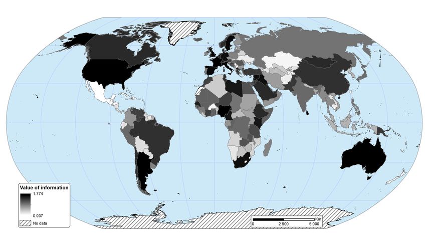
Figure 3 plots the origin-specific average of the value of information w(5)jt between 1980
and 2015 on a world map, revealing that there is no clear geographical pattern in the data,
with a substantial variability in the value of w(5)jt within, say, Latin America or Sub-Saharan
Africa.21 Figure 3 also reveals that high-income countries in Western Europe, North America
and Oceania are typically characterized by a high average value of w(5)jt , a pattern that will
be taken into account in the econometric analysis.
20
With N = 184, the upper bound of the value of information stands at ln(184) ≈ 5.2.
21
Notice that the range of values for w(5)jt is narrower in Figure 3 than in Table 1 as in the former we
are averaging across periods for each origin.
16Figure 3: Origin-specific average of the value of information w(5)jt
Source: Authors’ elaboration on Abel (2018).
The theory entails that the empirical counterpart π(r)jt , with r = {5, 10, 15, 20}, of the
return from information acquisition in (12) is simply given by the difference between the
empirical counterpart w(r)jt of the value of information and an (unknown) constant term.
This, in turn, implies that the evidence that we have just provided on the distribution of
w(5)jt , on its correlation with the proxies obtained using past migration flows over longer
time periods, and on the relevance of within-origin variability applies also to the proxy for
the return from information acquisition.
4 Econometric analysis
In this section, our objective is to test the empirical relevance of the value of information in
shaping migration decisions. To this end, we will augment a canonical gravity specification
of the determinants of migration flows with interactions of the empirical value of informa-
tion and income per capita at destination. The hypothesis that we will test, following our
theoretical model, is whether migrants respond more to changes in economic conditions at
destination when migrants attach a higher value to information. Hence, we expect the inter-
action between w(r)jt and income per capita in the destination country to be positive and
17significant.
4.1 Gravity equation with rational inattention
As a starting point, let us assume that information on the individual-specific values of
location-specific utilities can be costlessly acquired, i.e., λA = 0. In this case, we could
write the migration flows mjkt between an origin j and a destination k in the five-year
period starting in year t as:
mjkt = pjkt × njt × ζjkt (15)
where njt is the population residing in country of origin j in year t, ζjkt is an error term, and
the probability that destination k represents the utility-maximizing alternative for a migrant
from j is given by:
evjkt
pjkt = P vjlt
(16)
l∈A e
Replacing pjkt with the expression in (16), we can then rewrite equation (15) as:
" ! #
X
mjkt = exp vjkt − ln evjlt + ln(njt ) + ln(ζjkt ) (17)
l∈A
We assume that the deterministic component of utility vjkt in (17) follows:
ykt
vjkt = α ln (18)
τjkt
where ykt is real GDP per capita in destination k in year t, and τjkt ≥ 1 are dyadic and time-
varying iceberg migration costs. The specification in (18) entails that the semi-elasticity of
vjkt with respect to ykt is always equal to α, and independent of the value of the determinants
of dyadic migration costs τjkt . We specialize these dyadic costs as follows:
ln(τjkt ) = dkt + djt + djk + θ ln(sjkt + 1) (19)
where dkt , djt and djk represent destination-time, origin-time and origin-destination (dyadic)
dummies, and where ln(sjkt + 1) represents the logarithm of (one plus) the stock of j-born
18migrants residing in destination k in year t, as in Beine et al. (2011).22 The rich structure of
fixed effects included in (19) entails that we can only identify the effect of time-varying dyadic
variables, such as ln(sjkt + 1), or of destination-specific time-varying variables that produce
heterogeneous effects across origins or origin-destination pairs, while we cannot obtain an
estimate for α, which represents the elasticity of the bilateral migration rate with respect
to ykt . Using (19), we can rewrite the gravity equation that could be brought to the data
under the distributional assumptions introduced in Section 2 and when information is freely
available as follows:
mjkt = exp [dkt + djt + djk + θ ln(sjkt + 1) + ln(ζjkt )] (20)
The inclusion of destination-time dummies dkt would fail to absorb the effect of the time-
varying attractiveness of destination k, as this effect would be heterogeneous across origins
characterized by a different return from the acquisition of information when λA > 0. More
specifically, rational inattention means that bilateral flows from countries where migrants
have a higher return from acquiring information should be more responsive to variations in
the attractiveness of country k. Thus, we can extend the specification of the gravity equation
in (20) as follows:
mjkt = exp [dkt + djt + djk + β [ln(ykt ) × π(r)jt ] + θ ln(sjkt + 1) + ln(ζjkt )] (21)
where ln(ykt ) is the logarithm of GDP per capita in destination k in year t,23 and π(r)jt , with
r = {5, 10, 15, 20}, is the empirical counterpart of the return from information acquisition
for migrants from the origin j leaving in the five-year period starting in t. Given that
π(r)jt = w(r)jt − c(λA ), where c(λA ) is an unknown constant, the structure of fixed effects
implies that (21) is equivalent to:24
mjkt = exp [dkt + djt + djk + β [ln(ykt ) × w(r)jt ] + θ ln(sjkt + 1) + ln(ζjkt )] (22)
22
The data on the bilateral stock sjkt comes from Özden et al. (2011) between 1960 and 2000, with
interpolated values in between census years, and from United Nations Population Division (2015a) since
2005; the average and standard deviation of ln(sjkt + 1) over our sample of 263,008 observations stand at
2.25 and 2.95 respectively.
23
We use GDP per capita in 2010 USD from World Bank (2018); the average and standard deviation of
ln(ykt ) over our sample stand at 8.24 and 1.53 respectively.
24
The same equivalence would still hold even if π(r)jt = w(r)jt − c(λAt ), i.e., if the marginal cost of
acquiring information was varying over time.
19as the destination-time dummies dkt absorb the effect of −β[ln(ykt ) × c(λA )], given that
this part of the interaction term varies only at the destination-time level. The specification
that we can bring to the data is thus given by (22): if migrants are rationally inattentive,
then we should have that βb > 0. Since we have a large share of zeros (61.2 percent) in
our dependent variable mjkt , we estimate (22) using a Poisson pseudo-maximum-likelihood
estimator, following Santos Silva and Tenreyro (2006). More precisely, we employ the Stata
command ppmlhdfe developed by Correia et al. (2019a,b), which allows handling in a
computationally efficient way the large number of fixed effects in (22).
Dyadic dummies djk in (22) allow us to purge the estimate of the coefficient β of our
interaction term from the influence of time-invariant determinants of dyadic migration costs
that are hard to measure on a systematic basis, such as cultural distance (Spolaore and
Wacziarg, 2016) or linguistic proximity between countries that do not share the same lan-
guage (Adserà and Pytliková, 2015). For instance, an origin country j that is linguistically
close to many destinations will typically have a lower share of its past flows directed to the
main destination, i.e., higher value of w(r)jt and of the interaction term. The inclusion of
djk thus prevents unobserved dyadic determinants of migration flows from biasing β. b Origin-
P vjlt
year djt dummies control for the influence exerted on mjkt by ln l∈A e and ln(njt ) in
(17), while destination-year dkt dummies in (22) control for the time-varying attractiveness
of the destination k.
4.2 Main results
Table 3 reports the results obtained when bringing the gravity equation described in (22) to
the data. Each data column corresponds to one of the four variants of the empirical coun-
terpart for the value of information w(r)jt , with r = {5, 10, 15, 20}, for the origin country j
in the five-year period starting in year t.
20Table 3: Baseline results on the value of information
Dependent variable: mjkt
(1) (2) (3) (4)
Value of r 5 10 15 20
ln(ykt ) × w(r)jt 0.119∗∗∗ 0.145∗∗∗ 0.144∗∗∗ 0.161∗∗∗
(0.036) (0.040) (0.045) (0.055)
ln(sjkt + 1) 0.193∗∗∗ 0.192∗∗∗ 0.195∗∗∗ 0.196∗∗∗
(0.023) (0.023) (0.023) (0.023)
Observations 220,627 223,469 224,612 224,743
Pseudo-R2 0.963 0.963 0.963 0.963
w(r)jt (mean) 0.866 0.925 0.953 0.968
w(r)jt (s.d.) 0.532 0.523 0.518 0.515
djt , dkt and djk Yes Yes Yes Yes
Notes: ***, **, and * denote significance at the 1, 5, and 10 per-
cent levels, respectively. Clustered standard errors at the origin-time
level are reported in parentheses. The value of r denotes the num-
ber of years up to t that have been used to measure w(r)jt . All re-
gressions have been estimated with PPML using the Stata command
ppmlhdfe.
Source: Authors’ elaboration on Abel (2018), World Bank (2018),
Özden et al. (2011) and United Nations Population Division (2015a).
The estimates reveal that the coefficient βb of the interaction between GDP per capita
at destination and the time-varying origin-specific value of information is always positive
and significant at the 1 percent confidence level, consistently with the empirical relevance
of rational inattention in migration decisions.25 A one standard deviation increase in the
value of w(r)jt is associated with an increase in the elasticity of the bilateral migration rate
with respect to GDP per capita at destination ranging between 0.063, in column (1), to
0.083, in column (4). Going back to the example of China and Mexico that we introduced in
Section 3.2, the estimates in Table 3 entail that the elasticity for migration from China to any
destination between 1995 and 2000 was 0.160-0.216 higher than the corresponding elasticity
for migration from Mexico over the same time period. Similarly, the estimates also entail a
substantial variability over time for a given origin; for instance, the elasticity of migration out
25
Our analysis is fully robust to using gender-specific bilateral migration flows from Abel (2018); results
are available from the Authors upon request.
21of Ecuador increased by 0.069-0.093 between the early 1980s and the early 2000s,26 following
a substantial diversification of the main destinations for Ecuadorian migrants (Bertoli et al.,
2011).
The lower responsiveness of bilateral migration flows originating from countries where
migrants have stronger priors emerging from Table 3 could reflect the fact that a lower
value of information induces migrants (i) to invest less in information acquisition across all
destinations, or (ii ) to selectively disregard some destinations that are a priori very unlikely
to represent their preferred destinations, or (iii ) both. The analysis of the independent
consumer problem by Caplin et al. (2019), where a consumer has to select one good from a
choice set, with the utilities associated to the various alternatives being independent, reveals
that the optimal strategy of the consumer is to acquire information only about alternatives
that are characterized by a probability to maximize consumer’s utility that is above an
endogenous threshold. Let dzero (5)jkt be a dummy signaling a zero migration from j to
k in the five years up to year t. We have that 57.9 percent of the observations in our
sample correspond to origin-destination dyads with a zero flow in the recent past, and the
migration flows for these dyads could be less sensitive to variations in economic conditions
at destination, as migrants from j could exclude destination k from their (time-varying)
consideration sets when dzero (5)jkt = 1.
26
The value of w(5)ECU1980 stood at 0.168, increasing to w(5)ECU2000 = 0.744.
22Table 4: Zero past flows reduce responsiveness of flows to GDP per capita at destination
Dependent variable: mjkt
(1) (2) (3)
Value of r 5 5 5
ln(ykt ) × dzero (5)jkt -0.030∗∗∗ -0.028∗∗∗
(0.007) (0.007)
ln(ykt ) × w(r)jt 0.117∗∗∗ 0.119∗∗∗
(0.036) (0.036)
ln(sjkt + 1) 0.192∗∗∗ 0.185∗∗∗ 0.193∗∗∗
(0.025) (0.023) (0.023)
Observations 220,627 220,627 220,627
Pseudo-R2 0.963 0.964 0.963
w(r)jt (mean) 0.866 0.866 0.866
w(r)jt (s.d.) 0.532 0.532 0.532
djt , dkt and djk Yes Yes Yes
Notes: ***, **, and * denote significance at the 1, 5, and 10
percent levels, respectively. Clustered standard errors at the
origin-time level are reported in parentheses. The value of r
denotes the number of years up to t that have been used to
measure w(r)jt . dzero (5)jkt is a dummy equal to 1 if mjkt−5 =
0, and 0 otherwise. All regressions have been estimated with
PPML using the command ppmlhdfe.
Source: Authors’ elaboration on Abel (2018), World Bank
(2018), Özden et al. (2011) and United Nations Population Di-
vision (2015a).
Table 4 confirms that this is indeed the case: the elasticity with respect to GDP per
capita at destination is 0.030 points lower for origin-destination dyads characterized by zero
flows over the previous five years. However, this does not explain the role played by the value
of information in our baseline results, as our coefficient of interest is only marginally reduced
when introducing the additional interaction between dzero (5)jkt and ln(ykt ), as a comparison
of the second and of the third data column in Table 4 reveals.27
27
This also applies when using data over the previous 10, 15 or 20 years to identify origin-destination
pairs with past zero flows; results are available from the Authors upon request.
234.3 Threats to our interpretation
The interpretation that we have provided of the estimates in Table 3 is threatened by a
possible incorrect specification of location-specific utility in (18). More precisely, migration
decisions could be subject to binding liquidity constraints, which could influence migrants’
ability to respond to variations in economic conditions at destination even though they are
able to costlessly observe them. Furthermore, location-specific utility might not be additively
separable in ykt and in τjkt , so that the semi-elasticity of vjkt with respect to ykt could be a
function of the determinants of dyadic migration costs τjkt , e.g., the marginal utility of income
might be a function of dyadic migration costs, or it might depend on migrants’ individual
characteristics such as education. Similarly, the specification of the gravity equation in (22)
is consistent with a time-varying cost of information acquisition c(λA ), while it maintains
that this does not vary across origins, but the cost of information acquisition could vary at
the origin or at the dyadic level, possibly biasing our estimate of β.
We provide evidence here that our empirical evidence is robust to a more flexible speci-
fication of the deterministic component of utility that allows the responsiveness of bilateral
migration flows with respect to variations in economic conditions at destination to be het-
erogeneous across origins or across origin-destination pairs.
4.3.1 Liquidity constraints
Figure 3 in Section 3.2 above revealed that the empirical counterpart w(5)jt for the value
of information is higher in some geographical areas where most high-income countries are
concentrated. If we rely on the classification by income groups from the World Bank, we
have that the average value of w(5)jt stands at 1.088 for the high-income origin countries,
while it is equal to 0.805 for the other origin countries in our sample.28 Migration decisions
can be subject to binding liquidity constraints (see, for instance, Clemens, 2014, Angelucci,
2015, Bazzi, 2017 and Dao et al., 2018), which entail that the set of affordable destinations
is smaller than the choice set (Marchal and Naiditch, 2019), and hence this pattern in the
data poses a threat to our interpretation of the results in Table 3. Migrants from lower-
income countries might not value information less, but (because of liquidity constraints)
28
The classification by the World Bank is available on an yearly basis since 1989; we use the clas-
sification for year t since 1990, and the earliest available classification for previous years for each ori-
gin. Source: datahelpdesk.worldbank.org/knowledgebase/articles/906519-world-bank-country-and-lending-
groups (last accessed on January 22, 2019).
24they might be less able to react to variations in economic conditions at destination and their
past distribution could be more concentrated in the main (affordable) destination. Thus,
the positive and significant coefficient for the interaction term in Table 3 might be driven by
liquidity constraints rather than by rational inattention.
Table 5: Heterogeneity by income group
Dependent variable: mjkt
(1) (2) (3) (4)
Value of r 5 10 15 20
ln(ykt ) × w(r)jt 0.119∗∗∗ 0.140∗∗∗ 0.139∗∗∗ 0.159∗∗∗
(0.036) (0.040) (0.045) (0.056)
ln(ykt ) ×dlow
jt -0.170∗ -0.145 -0.145 -0.131
(0.098) (0.098) (0.102) (0.104)
ln(ykt ) ×dl.jt middle -0.225∗∗ -0.201∗∗ -0.213∗∗ -0.208∗∗
(0.092) (0.091) (0.096) (0.097)
ln(ykt ) ×du.
jt
middle
-0.043 -0.032 -0.049 -0.040
(0.085) (0.085) (0.090) (0.090)
ln(sjkt + 1) 0.201∗∗∗ 0.200∗∗∗ 0.203∗∗∗ 0.204∗∗∗
(0.023) (0.023) (0.023) (0.023)
Observations 216,027 218,869 220,012 220,143
Pseudo-R2 0.964 0.964 0.963 0.963
w(r)jt (mean) 0.867 0.931 0.965 0.981
w(r)jt (s.d.) 0.527 0.519 0.515 0.511
djt , dkt and djk Yes Yes Yes Yes
Notes: ***, **, and * denote significance at the 1, 5, and 10 percent
levels, respectively. Clustered standard errors at the origin-time level
are reported in parentheses. dlow l. middle
jt , djt , and du.
jt
middle
are dummies
taking the value of 1 if the origin j is classified by the World Bank as a
low, lower middle-income or upper middle-income country respectively
in year t, and 0 otherwise. The value of r denotes the number of years
up to t that have been used to measure w(r)jt . All regressions have
been estimated with PPML using the Stata command ppmlhdfe.
Source: Authors’ elaboration on Abel (2018), World Bank (2018),
Özden et al. (2011) and United Nations Population Division (2015a).
We thus bring to the data an extended version of the gravity equation in (21), where
we allow for a heterogeneous effect of ln(ykt ) across groups of origins characterized by a
25different level of income, differentiating between low-income, lower middle income, upper
middle income and high-income countries, with the latter representing the omitted category.
The estimates in Table 5 reveal that the elasticity of the migration rate with respect to ykt
is significantly higher (or at least not lower) for origins classified as high-income countries
in year t, consistently with the idea that liquidity constraints can reduce the responsiveness
of migration flows to the time-varying attractiveness of a destination country. However, this
does not influence either the size nor the significance of the coefficient for our interaction
effect, thus dismissing the concern that the values of βb in Table 3 were picking up a spurious
correlation between w(r)jt and the income group to which the origin j belonged in year t.29
4.3.2 More flexible responsiveness to economic conditions at destination
Do the results presented in Table 3 survive once we allow for a more general functional
form of the deterministic component of utility vjkt , or for differences across origins in the
cost of acquiring information on the attractiveness of the various destinations? For instance,
one could plausibly imagine that migrants from countries with larger past migration flows,
with stronger networks at destination or facing lower moving costs could more easily acquire
information on the attractiveness of the alternative destinations. This could explain our
results if origin countries that are characterized by a higher value of information also face a
lower cost of acquiring information.30 We address this relevant empirical concern introducing
an additional interaction term, between ln(ykt ) and the logarithm of the total emigration rate
for the origin j in the r years up to year t, with r taking the same value that is used to measure
the value of information w(r)jt . The estimated coefficient for this additional interaction term
is always positive, and significant in three out of the four data columns in Table 6, in line
with the idea that larger past migration flows reduce the cost of acquiring information on
the attractiveness of the alternative destinations.31 However, the inclusion of the additional
29
We obtain similar results when considering a time-invariant income classification of the origin j, or
when introducing an interaction between ln(ykt ) and ln(yjt ); results are available from the Authors upon
request.
30
Notice that the theoretical expression for the value of information in (14), as well as its empirical
counterparts, are insensitive to the scale of past migration flows, as they only depend on the distribution of
migrants across destinations.
31
An alternative, but not mutually exclusive, explanation is that past migrants help relaxing liquidity
constraints at origin through the remittances that they send back to their origin countries, thus increasing,
as suggested by Table 5, the responsiveness of bilateral migration flows with respect to varying economic
conditions at destination.
26You can also read