Chapitre 3 - Notions sur les instructions d'un ordinateur - Univ ...
←
→
Page content transcription
If your browser does not render page correctly, please read the page content below
2 LMD    Architecture des ordinateurs                 Chap. 3              Univ. Tiaret     Mr A. CHENINE

         Chapitre 3 – Notions sur les instructions d’un ordinateur

    1. Langage haut niveau (HLL), assembleur, langage machine

                                              Fig. 1 software levels
Programs that convert a user’s program written in some language to another language are called translators.

                                            Fig. 2 translation process

                                                                                                              31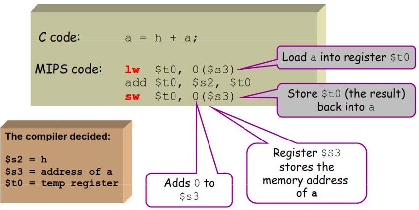
2 LMD Architecture des ordinateurs Chap. 3 Univ. Tiaret Mr A. CHENINE
Compilation
interpretation
The compiler translates the C text into ‘machine code’ for the processor
– Machine code is a set of consecutive memory words, encoding instructions for the processor.
– Machine code are binary words. In case of the MIPS processor, each instruction is 32 bits
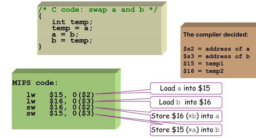
Translation examples
32
2 LMD   Architecture des ordinateurs   Chap. 3   Univ. Tiaret   Mr A. CHENINE

                                                                                33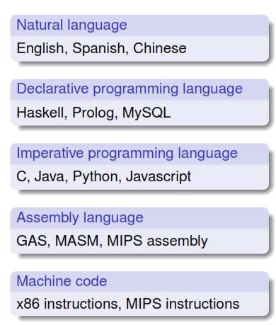
2 LMD Architecture des ordinateurs Chap. 3 Univ. Tiaret Mr A. CHENINE
Assembler
Three types of statements in assembly language
Typically, one statement should appear on a line
1. Executable Instructions
Generate machine code for the processor to execute at runtime
Instructions tell the processor what to do
2. Pseudo-Instructions and Macros
Translated by the assembler into real instructions
Simplify the programmer task
3. Assembler Directives
Provide information to the assembler while translating a program
Used to define segments, allocate memory variables, etc.
Non-executable: directives are not part of the instruction set
Instructions
Assembly language instructions have the format:
[label:] mnemonic [operands] [#comment]
Label: (optional)
Marks the address of a memory location, must have a colon
Typically appear in data and text segments
Mnemonic
Identifies the operation (e.g. add, sub, etc.)
Operands
Specify the data required by the operation
Operands can be registers, memory variables, or constants
Most instructions have three operands
L1: addiu $t0, $t0, 1 #increment $t0
Comments are very important!
Explain the program's purpose
When it was written, revised, and by whom
Explain data used in the program, input, and output
Explain instruction sequences and algorithms used
Comments are also required at the beginning of every procedure
Indicate input parameters and results of a procedure
Describe what the procedure does
Single-line comment
Begins with a hash symbol # and terminates at end of line
34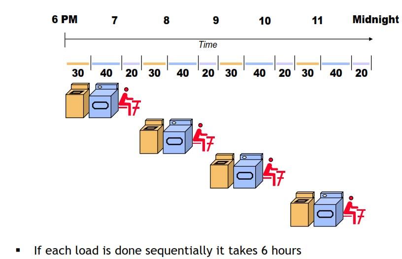
2 LMD     Architecture des ordinateurs                   Chap. 3               Univ. Tiaret      Mr A. CHENINE

    2. THE ASSEMBLY PROCESS [2]
        In the following sections we will briefly describe how an assembler works. Although each machine has a
different assembly language, the assembly process is sufficiently similar on different machines that it is possible to
describe it in general.

2.1 Two-Pass Assemblers

         Because an assembly language program consists of a series of one-line statements, it might at first seem
natural to have an assembler that read one statement, then translated it to machine language, and finally output the
generated machine language onto a file, along with the corresponding piece of the listing, if any, onto another file.
This process would then be repeated until the whole program had been translated. Unfortunately, this strategy does not
work.

          Consider the situation where the first statement is a branch to L. The assembler cannot assemble this statement
until it knows the address of statement L. Statement L may be near the end of the program, making it impossible for
the
assembler to find the address without first reading almost the entire program. This difficulty is called the forward
reference problem, because a symbol, L, has been used before it has been defined; that is, a reference has been made
to a symbol whose definition will only occur later.

Forward references can be handled in two ways. First, the assembler may in fact read the source program twice. Each
reading of the source program is called a pass; any translator that reads the input program twice is called a two-pass
translator.

On pass one, the definitions of symbols, including statement labels, are collected and stored in a table. By the time the
second pass begins, the values of all symbols are known; thus no forward reference remains and each statement can be
read, assembled, and output. Although this approach requires an extra pass over the input, it is conceptually simple.
The second approach consists of reading the assembly program once, converting ing it to an intermediate form, and
storing this intermediate form in a table in memory. Then a second pass is made over the table instead of over the
source program.

If there is enough memory (or virtual memory), this approach saves I/O time. If a listing is to be produced, then the
entire source statement, including all the comments, has to be saved. If no listing is needed, then the intermediate form
can be reduced to the bare essentials.

Either way, another task of pass one is to save all macro definitions and expand the calls as they are encountered. Thus
defining the symbols and expanding the macros are generally combined into one pass.

2.2 Pass One
The principal function of pass one is to build up a table called the symbol table, containing the values of all symbols.
A symbol is either a label or a value that is assigned a symbolic name by means of a pseudoinstruction such as

        ret EQU 1

2.3 Pass Two
The function of pass two is to generate the object program and possibly print the assembly listing. In addition, pass
two must output certain information needed by the linker for linking up procedures assembled at different times into a
single executable file.

    3. Hardware
                                                                                                                         35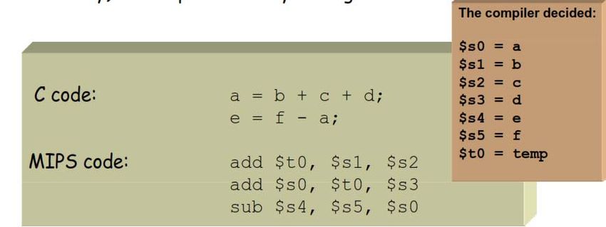
2 LMD   Architecture des ordinateurs                 Chap. 3              Univ. Tiaret    Mr A. CHENINE

   3.1 Arithmetic operations
   3.1.1 Addition/Subtraction

                                Fig.3 Block diagram for addition/subtraction (From [1])

Logisim implementation

Control signals are needed to control whether or not the complementer is used, depending on whether the
operation is addition or subtraction.

                                                                                                          36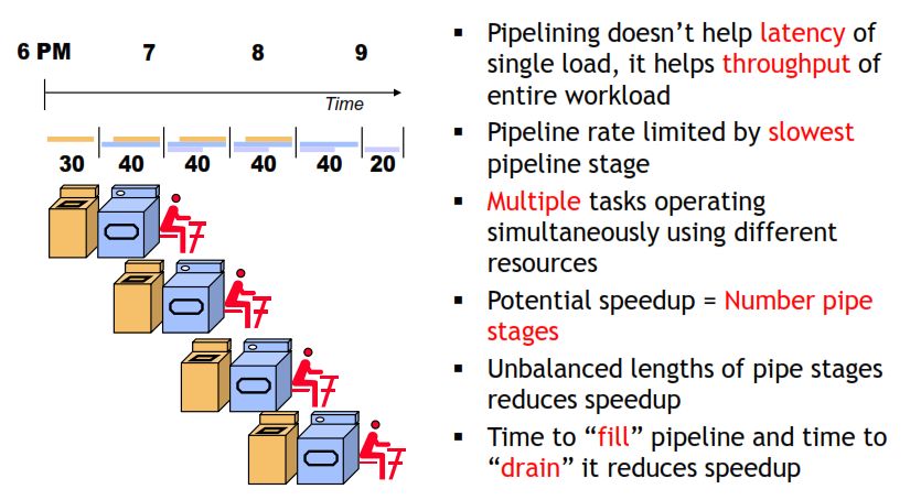
2 LMD   Architecture des ordinateurs                Chap. 3              Univ. Tiaret   Mr A. CHENINE

                                             Fig.4 Serial addition

  3.1.2 Unsigned Multiplication
  complex operation, the steps are:

                                Fig.5 Multiplication of Unsigned Binary Integers

  1. Multiplication involves the generation of partial products, one for each digit in the multiplier. These
     partial products are then summed to produce the final product.

  2. The partial products are easily defined. When the multiplier bit is 0, the partial product is 0. When
     the multiplier is 1, the partial product is the multiplicand.

  3. The total product is produced by summing the partial products. For this operation, each successive
     partial product is shifted one position to the left relative to the preceding partial product.

  4. The multiplication of two n-bit binary integers results in a product of up to 2n bits in length
     (e.g., 11 * 11 = 1001).

                                                                                                             37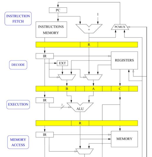
2 LMD   Architecture des ordinateurs                Chap. 3             Univ. Tiaret   Mr A. CHENINE


                                   Fig.6 a. Multiplication diagram b. Example

Logisim implementation

                                                                                                       38
2 LMD   Architecture des ordinateurs                 Chap. 3              Univ. Tiaret   Mr A. CHENINE

                                    Fig.7 Flowchart for unsigned Multiplication

Another method for multiplication

                                    Fig. 8 Multiplication of two 2-bit numbers


                                                                                                         39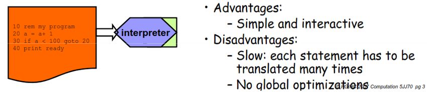
2 LMD Architecture des ordinateurs Chap. 3 Univ. Tiaret Mr A. CHENINE
Fig. 9 Logic circuit of 2x2-bit numbers
Question:
Compare fig. 9 and fig. 6.
4. Pipeline
Technique utilisée pour optimiser le temps d’exécution d’un processus répétitif.
Si le temps d’exécution d’un processus est T, l’exécution séquentielle de m processus prend un
temps m*T.
402 LMD Architecture des ordinateurs Chap. 3 Univ. Tiaret Mr A. CHENINE
412 LMD Architecture des ordinateurs Chap. 3 Univ. Tiaret Mr A. CHENINE
422 LMD Architecture des ordinateurs Chap. 3 Univ. Tiaret Mr A. CHENINE
432 LMD Architecture des ordinateurs Chap. 3 Univ. Tiaret Mr A. CHENINE
Le pipeline
Le temps passé par une instruction dans un étage est appelé (temps de) cycle processeur
La longueur d’un cycle est déterminée par l’étage le plus lent.
Souvent égal à un cycle d’horloge, parfois 2
L’idéal est d’équilibrer la longueur des étages du pipeline
Sinon le étages les plus rapides ‘attendent’ les plus lents
Pas optimal
Insertion de registres intermédiaires entre les étages (Registres pipeline)
Exemple avec un pipeline à 5 étages :
1. Lecture de l’instruction (IF)
2. Décodage de l’instruction (ID)
3. Exécution de l’instruction (EX)
4. Accès mémoire (MEM)
5. Ecriture du résultat (WB)
442 LMD Architecture des ordinateurs Chap. 3 Univ. Tiaret Mr A. CHENINE
452 LMD Architecture des ordinateurs Chap. 3 Univ. Tiaret Mr A. CHENINE
462 LMD Architecture des ordinateurs Chap. 3 Univ. Tiaret Mr A. CHENINE
1. Lecture de l’instruction (IF)
La prochaine instruction à exécuter est chargée à partir de la case mémoire pointée par le compteur
de programme (PC) dans le registre d'instruction RI.
Le compteur de programme est incrémenté pour pointer sur l'instruction suivante.
2. Décodage de l’instruction (ID)
Cette étape consiste à préparer les arguments de l'instruction pour l'étape suivante (UAL) où ils seront
utilisés. Ces arguments sont placés dans deux registres A et B.
Si l'instruction utilise le contenu d’un ou deux registres, ceux-ci sont lus et leurs contenus sont rangés
dans A et B.
Si l'instruction contient une valeur immédiate, celle-ci est étendue (signée ou non signée) à 16 bits et
placée dans le registre B.
Pour les instructions de branchement avec offset, le contenu de PC est rangé en A et l'offset étendu
dans B.
Pour les instructions de branchement avec un registre, le contenu de ce registre est rangé en A et B
est rempli avec 0.
Les instructions de rangement mettent le contenu du registre qui doit être transféré en mémoire dans
le registre C.
3. Exécution de l’instruction (EX)
472 LMD Architecture des ordinateurs Chap. 3 Univ. Tiaret Mr A. CHENINE
Cette étape utilise l’UAL pour combiner les arguments. L'opération réalisée dépend du type de l'instruction.
Instruction arithmétique ou logique (ADD, AND et NOT)
Les deux arguments contenus dans les registres A et B sont fournis à l'UAL pour calculer le résultat.
Instruction de chargement et rangement (LW et SW)
Le calcul de l'adresse est effectué à partir de l'adresse provenant du registre A et de l'offset contenu
dans le registre B.
Instruction de branchement
Pour les instructions contenant un offset, addition avec le contenu du PC.
Pour les instructions utilisant un registre, le contenu du registre est transmis.
4. Accès mémoire (MEM)
Cette étape est uniquement utile pour les instructions de chargement et de rangement.
Pour les instructions arithmétiques et logiques ou les branchements, rien n'est effectué. L'adresse du
mot mémoire est contenue dans le registre R.
Dans le cas d'un rangement, la valeur à ranger provient du registre C.
Dans le cas d'un chargement, la valeur lue en mémoire est mise dans le registre R pour l'étape
suivante.
482 LMD Architecture des ordinateurs Chap. 3 Univ. Tiaret Mr A. CHENINE
5. Ecriture du résultat (WB)
Le résultat des opérations arithmétiques et logiques est rangé dans le registre destination.
La valeur lue en mémoire par les instructions de chargement est aussi rangée dans le registre
destination.
Les instructions de branchement rangent la nouvelle adresse dans PC.
492 LMD Architecture des ordinateurs Chap. 3 Univ. Tiaret Mr A. CHENINE
Reference
[1] William Stallings, Computer organization and architecture, Designing for Performance, tenth edition,
[2] Tanenbaum A.S., Austin T. - Structured computer organization-Pearson (2013)
50You can also read