Classification of Soccer and Basketball Players' Jumping Performance Characteristics: A Logistic Regression Approach
←
→
Page content transcription
If your browser does not render page correctly, please read the page content below
sports
Article
Classification of Soccer and Basketball Players’
Jumping Performance Characteristics: A Logistic
Regression Approach
Christos Chalitsios *, Thomas Nikodelis , Vassilios Panoutsakopoulos , Christos Chassanidis
and Iraklis Kollias
 Biomechanics Laboratory, Department of Physical Education and Sports Sciences, Aristotle University
 of Thessaloniki, 54124 Thessaloniki, Greece
 * Correspondence: cchalits@phed.auth.gr; Tel.: +30-23-1099-2202

 Received: 19 March 2019; Accepted: 2 July 2019; Published: 4 July 2019

 Abstract: This study aimed to examine countermovement jump (CMJ) kinetic data using logistic
 regression, in order to distinguish sports-related mechanical profiles. Eighty-one professional
 basketball and soccer athletes participated, each performing three CMJs on a force platform. Inferential
 parametric and nonparametric statistics were performed to explore group differences. Binary logistic
 regression was used to model the response variable (soccer or not soccer). Statistical significance
 (p < 0.05) was reached for differences between groups in maximum braking rate of force
 development (RFDDmax , U79 = 1035), mean braking rate of force development (RFDDavg , U79 = 1038),
 propulsive impulse (IMPU , t79 = 2.375), minimum value of vertical displacement for center of mass
 (SBCMmin , t79 = 3.135), and time difference (% of impulse time; ∆T ) between the peak value of
 maximum force value (FUmax ) and SBCMmin (U79 = 1188). Logistic regression showed that RFDDavg ,
 impulse during the downward phase (IMPD ), IMPU , and ∆T were all significant predictors. The model
 showed that soccer group membership could be strongly related to IMPU , with the odds ratio being
 6.48 times higher from the basketball group, whereas RFDDavg , IMPD , and ∆T were related to basketball
 group. The results imply that soccer players execute CMJ differently compared to basketball players,
 exhibiting increased countermovement depth and impulse generation during the propulsive phase.

 Keywords:    vertical ground reaction force;             sport specificity;   impulse;    rate of force
 development; biomechanics

1. Introduction
      The main focus of athletic training at the competitive level is to improve the athlete’s specific
and relevant abilities that are essential to the sport. Players in sports such as basketball and soccer
usually perform repetitive tasks such as jumps, rapid changes of direction, and intense accelerations
or decelerations [1,2]. The execution of these movements is primarily based on the capacity of the
musculoskeletal system to produce power and impulse [3]. Vertical jumping is a fundamental skill
that may distinguish top performers in both sports and, for that reason, it represents a training goal
for strength and conditioning coaches. Various training models are usually adopted by professionals
in order to increase that capacity [4,5]. The unloaded countermovement jump (CMJ) without arm
swing is one of the most popular tests to assess lower limb performance [6]. Studies have shown
that the observed increase in jump height after training represents a valid and positively contributing
factor to the improvement of sporting performance [7,8]. Yet, assessing athletic performance only in
terms of jump height is somewhat simplistic as it does not offer an inside view of the mechanisms
defining performance.

Sports 2019, 7, 163; doi:10.3390/sports7070163                                   www.mdpi.com/journal/sports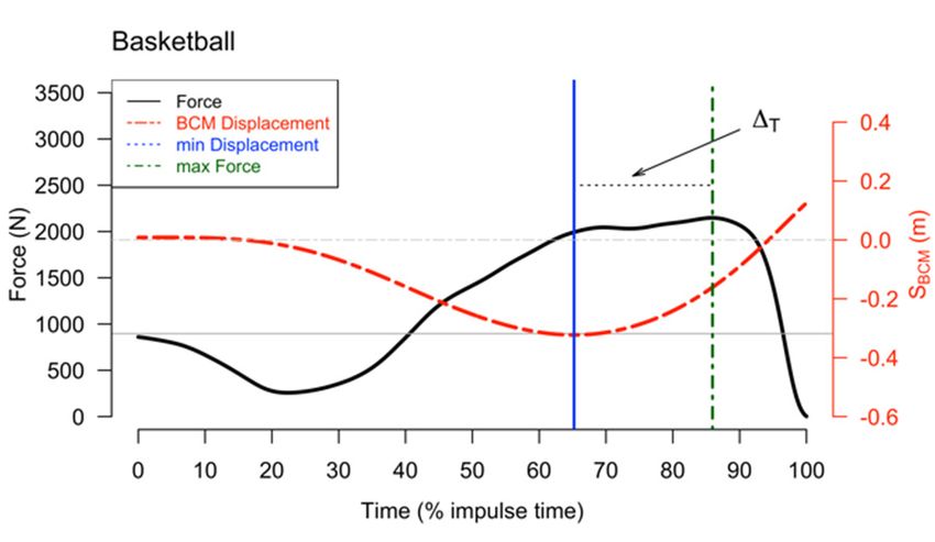
Sports 2019, 7, 163                                                                                     2 of 9

      Vertical jumping force–time characteristics are quite different between soccer and basketball [9].
The main difference is the frequency and timing in which athletes are called upon to perform jumps.
In soccer, the playing fields are larger and there is no time restriction for specific game actions to
occur, thus, there is more time for prediction and reaction, while for basketball, the opposite is true.
These differences may affect the way that players regulate their jumping strategy and trigger the
adoption of different training protocols.
      Indeed, training background has an effect on the pattern of vertical force production [10]. The use
of principal component analysis to explore force–time series during vertical jumping showed that the
extracted components could discriminate different sporting backgrounds. More specifically, it revealed
that sport-specific kinetic profiles exist and they are based on the utilization of the force and temporal
parameters in a sport background combination [9,11–13]. Although principal component analysis has
been used extensively for exploring the underlying structure of observed patterns between different
groups of interest, this method aims to analyze each variable under the assumption that features with
high variance are more likely to achieve a good split between the classes. This technique presents
a geographical representation of the trend towards a principal component in the n-dimensional space.
Nevertheless, it does not provide a numerical expression for the possibility of an individual to belong
in a sports group according to the features that comprise his/her performance.
      The adoption of a simple, yet powerful-enough classification model, which considers every
independent variable impact on the response variable, may provide alternative insights into the
differences among examined populations and, more importantly, provide interpretable and usable
results. One such method is logistic regression. This statistical technique is often used for the probability
estimation of the dependent variable from one or more predictor variables, and presents a useful and
efficient tool to assess independent variable contributions to a binary outcome. Classifying the overall
mechanical profile of a jump execution in such a way, regardless of the statistical differences that may
exist in individual parameters, may prove useful for training, recruiting, and even injury-preventing
purposes. In fact, there are already such examples in gait biomechanics [14].
      Furthermore, up until now, such classification analysis of jumping mechanical profiles has not been
conducted, at least to the extent of our knowledge and after intensive research. Instead, the comparative
literature is limited to descriptive differences on selected variables of CMJ. For example, soccer and
basketball players do not differ significantly in terms of jump height [15]. Such results do not offer
useful information to strength coaches about the underlying kinetic mechanisms of jumping strategy
that may be imposed by the sport specificity. The purpose of the present study was to combine CMJ
kinetic data with the statistical classification tool of logistic regression in order to test the hypothesis
that different mechanical profiles are sports-dependent.

2. Materials and Methods

2.1. Study Design
     A cross-sectional design was adopted to explore various features of vertical ground reaction force
(GRFV )–time curve during CMJ. Statistical inference and classification modeling were used to investigate
the differences that could be identified due to the sporting background. Various biomechanical factors
on which jumping performance is based were considered in both sports groups.

2.2. Participants
     In this study, 81 male adult athletes performing in top-level professional leagues in Greece for
basketball (n = 39, age 28.9 ± 3.5 years, body mass 97.4 ± 10.6 kg, height 1.97 ± 0.08 m) and soccer (n = 42,
age 26.4 ± 4.3 years, body mass 77.0 ± 9.3 kg, height 1.82 ± 0.07 m) were tested. Participants were
inspected for any muscular dysfunction that may have occurred during the three months before
testing. In any case, athletes with typical injuries caused by impacts during practice or competition
had completely recovered at the time of the measurements. Testing took place during the last week
Sports 2019, 7, 163 3 of 9
of the pre-season, where the training volume was intentionally lower to minimize accumulating
fatigue. Participants abstained from team practice one day before testing. Prior to their participation,
all individuals signed informed consent forms regarding the risks and benefits of the investigation
according to the Institutional Ethics Committee Guidelines.
2.3. CMJ Testing
All participants performed a series of three CMJs on a triangular dual force plate system (k-Delta,
K-Invent Biomecanique, Orsay, France) that incorporated three 1D force sensors on each plate.
Before testing, participants carried out a 10 min standardized warm-up that consisted of slow pace
running on a treadmill for 6 min at a constant velocity of 2 m·s−1 without load or inclination and
combined with static and dynamic stretching. After a thorough explanation and physical demonstration,
each individual performed the test based on standardized instructions “to jump as high and as fast as
possible”. Three submaximal jumps on the force plates followed the warm-up, for checking technical
execution. All jumps were executed with hands at the akimbo position until landing and stabilization.
Each participant performed a total of three jumps without any restriction for countermovement depth.
A time interval of 1.5 min was set between trials to avoid any fatigue. The trial with the highest value
for jump height was further analyzed. All testing was performed between 16:00 and 18:00 pm.
2.4. Data Recording and Analysis
GRFV acquired from the force plate was sampled at 500 Hz and the force plate’s accompanying
software was used to obtain the raw data values. GRFV from each platform was summed to create
the total force–time signal. Raw data were filtered using a 2nd order Butterworth filter and the cutoff
frequency was set at 20 Hz. Force data were used to compute the variables for braking and propulsive
phases. The braking phase was defined from the initiation of the movement (force below 95% of body
weight) until the point where vertical displacement reached its minimum value. The propulsive phase
started immediately after the end of the braking phase until take-off. Jump height calculation was
derived using the impulse-momentum theorem [16]. Recorded data were used to calculate kinetic and
kinematic variables such as maximum braking rate of force development (RFDDmax ), mean braking rate
of force development (RFDDavg ), braking impulse (IMPD ), propulsive impulse (IMPU ), maximum force
value (FUmax ), mean value of force (FUavg ) over the propulsive phase, peak power (PUmax ), mean power
(PUavg ), the minimum value of vertical displacement (SBCMmin ), and the time difference (% of impulse
time) between the peak value of FUmax and SBCMmin (∆T ). All variables were expressed as units per body
mass, except for RFDDmax and RFDDavg . The value of SBCMmin was scaled to body height. All analyses
were stored using MATLAB (2015b, Mathworks, Natick, MA, USA) and Signal Processing Toolbox.
2.5. Statistical Analysis
Statistical procedures were performed with R v3.2.2 (R Foundation for Statistical Computing,
Vienna, Austria). The average value of the standard error of measurement (SEM) between the three
trials, concerning jump height, was 2.5 ± 1.1 cm, which accounts for ~2% of maximum hump height.
Distribution properties of the data were checked using the Shapiro–Wilk test. If distributions between
groups did not reject the null hypothesis of the normality test, an independent samples Student’s t-test
was applied over all variables to check for differences in the means between the two groups. If data
were not normally distributed, a Mann–Whitney U test was carried out. Cohen’s effect sizes d and r
were calculated and reported for parametric and nonparametric tests respectively.
Multivariable logistic regression analysis was performed to classify the binary outcome of group
membership (Basketball = 0, Soccer = 1). Classification threshold was set to 0.5. The logistic regression
model was estimated using a logit link function, assuming a binomial distribution for the outcomes.
Model development was based on a backward elimination strategy using the Akaike information
criterion (AIC) as a selection metric. The model with the lowest AIC was selected for further analysis.
Variance inflation was used for multicollinearity checking and variables that inflated above 5 wereSports 2019, 7, x FOR PEER REVIEW 4 of 9
Variance
Sports 2019,inflation
7, 163 was used for multicollinearity checking and variables that inflated above 5 were
4 of 9
removed. Goodness-of-fit was obtained based on the Stukel test [17,18]. The test is based on the null
hypothesis that there are no deviations from the logit link function. The logistic equation was solved
removed. Goodness-of-fit was obtained based on the Stukel test [17,18]. The test is based on the null
for each participant to determine into which group he would be classified. Discrimination ability was
hypothesis that there are no deviations from the logit link function. The logistic equation was solved
quantified based on the area under the curve (AUC) which measures the area under the receiver
for each participant to determine into which group he would be classified. Discrimination ability
operating characteristic (ROC) curve. An AUC value of 1 (100%) corresponds to perfect
was quantified based on the area under the curve (AUC) which measures the area under the receiver
discrimination and 0.5 (50%) to random chance. The application of a resampling technique is
operating characteristic (ROC) curve. An AUC value of 1 (100%) corresponds to perfect discrimination
recommended for the analysis of small sample sizes [19]. Thus, for the internal validation of the
and 0.5 (50%) to random chance. The application of a resampling technique is recommended for the
model, a bootstrap approach was carried out to estimate the performance of the classifier and to avoid
analysis of small sample sizes [19]. Thus, for the internal validation of the model, a bootstrap approach
overfitting [20]. For all statistical tests, an alpha level of 0.05 was set.
was carried out to estimate the performance of the classifier and to avoid overfitting [20]. For all
statistical
3. Results tests, an alpha level of 0.05 was set.
3. Results
Results revealed statistically significant differences in several of the examined variables.
Descriptive statistics are shown in Table 1. Statistical significance was reached in RFDDmax (U79 = 1035,
Results revealed statistically significant differences in several of the examined variables.
r = 0.88) and RFDDavg (U79 = 1038, r = 0.87), with soccer players exhibiting lower values compared to
Descriptive statistics are shown in Table 1. Statistical significance was reached in RFDDmax (U79 = 1035,
basketball players. Furthermore, significantly greater values were observed in IMPU (t79 = −2.375, d =
r = 0.88) and RFDDavg (U79 = 1038, r = 0.87), with soccer players exhibiting lower values compared to
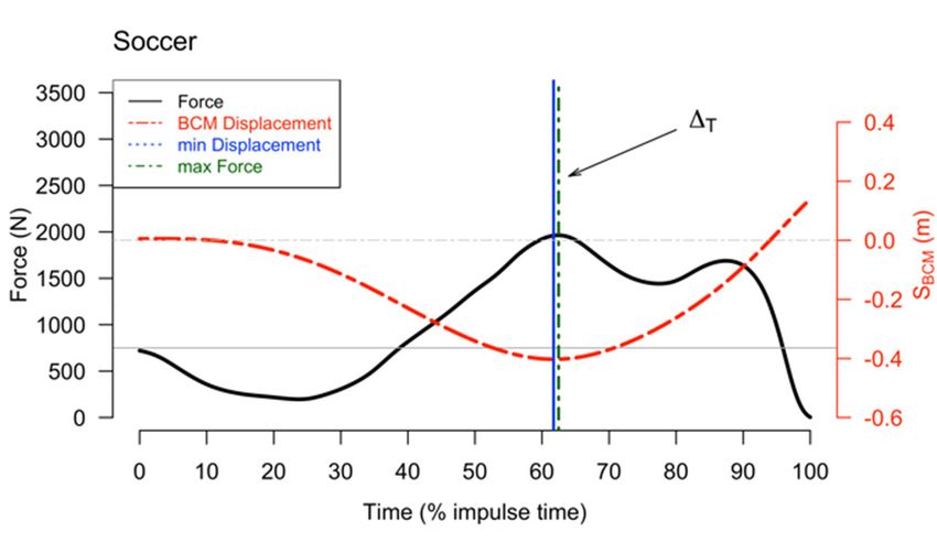
0.54) and SBCMmin (t79 = 3.135, d = 0.7), but not for ΔΤ (U79 = 1188, r = 0.69) in the soccer group, as shown
basketball players. Furthermore, significantly greater values were observed in IMPU (t79 = −2.375,
in Figure 1.
d = 0.54) and SBCMmin (t79 = 3.135, d = 0.7), but not for ∆T (U79 = 1188, r = 0.69) in the soccer group,
as shown in Figure 1.
Table 1. Descriptive statistics for the examined variables also used in the baseline model (mean ± SD,
CI 95% for the difference in means, p value).
Table 1. Descriptive statistics for the examined variables also used in the baseline model (mean ± SD,
CI 95% for the difference
Variable Basketball (n = p39)
in means, value).
Soccer (n = 42) Difference CI 95% p
Variable Mean ± SD
Basketball SoccerMean
(n = 42)± SD Difference Lower
CI 95% Upper p
RFDDmax (kN·s ) −1 (n = 39)
13.87 ± 5.11a 11.91 ± 5.31 1.96 0.08 4.02 0.041
RFDDavg (kN·s−1) 5.67±±SD
Mean 2.03a Mean4.67
± SD± 1.65 1.00 Lower0.04 Upper 1.67 0.038
IMP
RFDDmax (kN·s−1 )
D (N·s) 3.93
13.87 ± 5.11 a
± 0.54 11.91 4.04
± 5.31± 0.81 1.96−0.11 0.08−0.27 4.020.22 0.921
0.041
RFD (kN·s −1 ) 5.67 ± 2.03a ± 1.65± 0.45b
4.67 5.49 1.00−0.24 0.04−0.45 1.67−0.04 0.038
IMPUDavg (N·s) 5.25 ± 0.47 0.020
IMPD (N·s) 3.93 ± 0.54 4.04 ± 0.81 −0.11 −0.27 0.22 0.921
FUmaxIMP
(N·kg −1)
U (N·s)
24.47
5.25 ± 2.71
± 0.47 5.49 ±24.12
0.45b± 1.94 −0.240.35 −0.45−0.94 −0.041.10 0.991
0.020
FUmax
FUavg (N·kg −1)−1 )
(N·kg 24.47
19.97± 2.71
± 1.48 ± 1.94± 1.59
24.1219.89 0.35 0.08 −0.94−0.61 1.100.70 0.991
0.868
FUavg (N·kg−1 ) 19.97 ± 1.48 19.89 ± 1.59 0.08 −0.61 0.70 0.868
PUmax (W·kg−1)
PUmax (W·kg−1 )
53.94 ± 6.18
53.94 ± 6.18
55.10 ± 6.31
55.10 ± 6.31 1.16
1.16 −4.18
−4.18 1.261.26 0.348
0.348
PUavg (W·kg
PUavg (W·kg−1)−1
) 29.96
29.96 ± 3.79
± 3.79 30.8130.81
± 3.91± 3.91 −0.85−0.85 −2.60−2.60 0.780.78 0.344
0.344
SBCMmin −0.16 ± 0.04 −0.19−0.19
± 0.04±b
SBCMmin (m)(m) −0.16 ± 0.04 0.04b 0.03 0.03 0.01 0.01 0.040.04 0.002
0.002
∆T (%) 13.56 ± 9.3a 6.44 ± 8.3 7.12 1.78 14.13 0.000
ΔΤ (%) 13.56 ±a: 9.3 a 6.44 ± 8.3 7.12
Mann–Whitney U test, b: Independent t-test.
1.78 14.13 0.000
a: Mann–Whitney U test, b: Independent t-test.
(a) (b)
Figure
Figure1.1.Example
Example of of
characteristic difference
characteristic in Δin
difference ∆Ttypical
Τ: (a) force–time
: (a) typical curve of
force–time a basketball
curve player;
of a basketball
(b) typical
player; force–time
(b) typical curve curve
force–time of a soccer player.
of a soccer Vertical
player. lines
Vertical represent
lines thethemaximum
represent maximumvalue valueofof
countermovement
countermovementdepth depth(solid
(solidblue
blueline)
line)and
andmaximum
maximumvaluevalueof offorce
force(green
(green dashed
dashed line).
line). The
Thegrey
grey
horizontal
horizontallinelineindicates
indicatessubjects’
subjects’body
bodyweight,
weight,and
andthe
thedashed
dashedgreygreyhorizontal
horizontalline
lineindicates
indicatesthethezero
zero
value for
value for SSBCM
BCM. .Sports 2019, 7, 163 5 of 9
Sports 2019, 7, x FOR PEER REVIEW 5 of 9
Afterthe
After thevariable
variableelimination
eliminationprocess,
process,the
thefinal
finallogistic
logisticregression
regressionmodel
modelwas
wasbuilt
builtusing
usingonly
only
RFDDavg
RFD Davg,, IMP
IMPDD, ,IMPU, and
IMP ΔΤ (Table 2) where all predictors contributed significantly (p < 0.05). Stukel’s
U , and ∆T (Table 2) where all predictors contributed significantly (p < 0.05).
test for goodness-of-fit was
Stukel’s test for goodness-of-fit notwas
significant (p = 0.627).
not significant (p = 0.627).
Table2.2.The
Table Theoutput
outputofofthe
thelogistic
logisticregression.
regression.LogLogodds,
odds,odds
oddsratio,
ratio,and
andconfidence
confidenceintervals
intervals(95%
(95%CI)
CI)
forodds
for oddsratio
ratioand
andp pvalues
valuesofofthe
thecoefficients.
coefficients.
Variable
Variable Log Odds
Log Odds SE
SE Odds
Odds Ratio
Ratio CI 95% CI 95%p p
RFDDavg −1.194 0.33 0.3 (0.16–0.58) 0.000
RFDDavg −1.194 0.33 0.3 (0.16–0.58) 0.000
IMPD IMPD −2.639
−2.639 0.85
0.85 0.07
0.07 (0.01–0.37)(0.01–0.37)
0.002 0.002
IMPU IMPU 1.869
1.869 0.94
0.94 6.48
6.48 (1.02–41.1)(1.02–41.1)
0.047 0.047
ΔΤ ∆T −0.161
−0.161 0.03
0.03 0.85
0.85 (0.79–0.92)(0.79–0.92)
0.000 0.000
Note:
Note:Nagelkerke’s
Nagelkerke’s =20.506.
R2 R = 0.506.
Theproposed
The proposedmodel
modelwaswasable
abletotodiscriminate
discriminatethe
thegroups
groups(Figure
(Figure2)2)with
withan
anin-sample
in-sampleAUC
AUCofof
0.87. After bootstrap, the AUC value was 0.847.
0.87. After bootstrap, the AUC value was 0.847.
Figure2.2.Diagnostic
Figure Diagnosticplots
plotsofofthe
thelogistic
logisticregression
regressionmodel
modelpredicting
predictinggroup
groupmembership:
membership:(a) (a)Model’s
Model’s
AUC performance; (b) Scatterplot of the respective classes probability; (c) Histogram—basketball
AUC performance; (b) Scatterplot of the respective classes probability; (c) Histogram—basketball
probability
probability(cutoff
(cutoffthreshold,
threshold,dashed
dashedline);
line); (d)
(d)Histogram—soccer
Histogram—soccer probability
probability (cutoff
(cutoff threshold,
threshold,
dashed
dashedline).
line).
Exponentiation
Exponentiationofofthe loglog
the of of
odds to obtain
odds to obtainthe the
odds ratioratio
odds for the
for predictor variables
the predictor revealed
variables that
revealed
the odds ratio for soccer group membership increased by 6.48 times for every
that the odds ratio for soccer group membership increased by 6.48 times for every N·s increase UinN·s increase in IMP
during −1 increase in RFD
IMPU CMJ.
during OnCMJ.
the contrary,
On the for every 1kN·s
contrary, for every Davg ,in
1kN·s−1 increase theRFD
odds ratio of any observation
Davg, the odds ratio of any
toobservation
be classifiedtoasbesoccer player
classified as decreased
soccer player multiplicatively by 0.3 times. Similarly,
decreased multiplicatively for unit
by 0.3 times. increases
Similarly, for
and regarding the variables IMP
unit increases and regarding theDvariables and ∆ , the odds ratio of soccer group membership
T IMPD and ΔΤ, the odds ratio of soccer group membershipdecreased
multiplicatively by 0.07 andby
decreased multiplicatively 0.85
0.07times, respectively.
and 0.85 All four variables
times, respectively. All four of the regression
variables reached
of the regression
areached
Nagelkerke pseudo R 2 value of 0.506, suggesting that 50.6% of the total variance was explained by
a Nagelkerke pseudo R value of 0.506, suggesting that 50.6% of the total variance was
2
RFD Davg , IMP
explained , IMP
by DRFD and D∆, TIMP
U ,, IMP
Davg
. U, and ΔΤ.
4. Discussion
In this study, we aimed to establish a classification method to confirm the assumption that
features of GRFV during CMJ can discriminate athletes according to their sporting background. TheSports 2019, 7, 163 6 of 9
4. Discussion
In this study, we aimed to establish a classification method to confirm the assumption that features
of GRFV during CMJ can discriminate athletes according to their sporting background. The logistic
regression approach was preferred because it provides interpretable results and, at the same time,
it performs well enough in terms of predictive ability. The experimental results appear supportive of
the feasibility of the proposed method. Descriptive statistics showed that basketball players appeared
to produce significantly higher values for RFDDavg and ∆T , while soccer players showed significantly
higher values for IMPU and SBCMmin . These significant differences will be discussed in relation to the
logistic regression. The final model of logistic regression was built using only four variables out of the
full model. The selected variables were RFDDavg , IMPD , IMPU , and ∆T . Stukel’s goodness-of-fit failed
to reject the null hypothesis and showed no evidence of poor fit [21].
The bootstrapped AUC (0.847) value for the final model denotes that this relatively simple,
four-variable final model displayed very good predictive power for the distinction of the original
groups. The final model demonstrated that membership to the soccer group could be strongly related
to IMPU , with the odds ratio being 6.48 times higher from the basketball group. This implies that soccer
players used a different kinetic pattern during the execution of CMJ, based on generating high impulses
during the propulsive phase of the movement. This indication is in accordance with other studies
where participants that exhibited greater countermovement depth also achieved greater values in
IMPU [22,23] and, consequently, greater jump height values compared to others. This is also supported
by the paired comparisons for the selected variable.
The model also displayed that RFDDavg , IMPD , and ∆T were significant predictors
of group classification. The result that RFDDavg is associated with basketball players is
indicative of their muscle–tendon system’s capacity to develop force quickly during the
stretching phase of the stretch–shortening cycle [12] using a decreased countermovement depth.
Nevertheless, the aforementioned reference did not consider the unloading phase to be part of the
downwards impulse phase, thus introducing a bias to their calculations [16]. Ugrinowitch [10] also
proposed that athletes, in sports where time constraints are present, try to apply force with large
acceleration values in order to maximize jumping height.
Another interesting finding is that the increasing trend of ∆T value was related to the basketball
group. The time used for the execution of the jump has been shown to affect the mechanical properties
of performance even through verbal instructions [24]. Moreover, it seems that for basketball players,
the moment of reaching minimum displacement (SBCMmin ) is more distal from the time point of FUmax
application compared to soccer players. The jumps that basketball players usually perform during
practice or in competition are not maximal as they are constrained to act before opponents. For example,
consecutive rebounding, block and rebound, and shooting to beat the buzzer are totally different
from a timing perspective compared to jumps in soccer, and especially regarding the time coupling
interaction with the opponent.
This leads to jumps that are executed quickly, without large countermovement action, and with
high dependence on force production from the ankle plantar flexors [25,26]. Indeed, Salles et al. [22]
proposed that the appearance of FUmax close to the end of the propulsive phase during CMJ is related to
increased calf muscle activation. At that specific point in time, hip and knee joints are already extended
due to decreased countermovement and short duration of push-off, preventing their extensors reaching
maximal activation and from thus producing maximum force and impulse [27,28]. The joint that can
continue the contribution to the force production is the ankle, as it is not yet fully plantar-flexed [22].
Soccer players, on the other hand, seem to utilize this specific parameter (∆T ) in the opposite
way. It seems that for soccer players, the time points of FUmax and SBCMmin are occurring almost at
the same time, and they consistently performed CMJs with greater depth in comparison to basketball
players. Bobbert et al. [28] showed that the lower the position of the center of mass was before the
upward push-off phase, the later the activation of plantar flexors occurred. This was indicative of
greater activation for knee and hip flexors. Maximal jumping in soccer is a crucial factor for claimingSports 2019, 7, 163 7 of 9
the ball. Soccer players have more time at their disposal for performing a vertical jump due to the
larger distances they are called to act upon in a soccer field. The aforementioned features may be the
sport specific regulators of that variable (∆T ).
Furthermore, soccer players exhibit larger push-off durations and IMPU in order to maximize
their jump height. Fukashiro and Komi [25] stated that this kinetic pattern is associated mainly with
energy contribution from the hip/knee joint bi-articular muscles and minimal activity from muscles in
the ankle. Similar findings from Vanrenterghem et al. [29] demonstrate that the ankle joint contributes
only 23% of the necessary energy generation of a maximal jump. A connection between increasing the
total work in order to increase jump height and the increased contribution from the large proximal
muscles has also been reported in the literature [30]. Recently, this statement has been associated
with increases in hip and knee peak angles, indicating transitions from an ankle-centered strategy to
a hip/knee movement strategy [26].
The confidence interval for the odds ratio (1.02–41.1) of IMPU is wide. Such wide confidence
intervals often occur due to small sample sizes, explanatory variables with a narrow distribution,
or data sparsity. Sparse data are often present in research settings, especially in binary logistic regression
which has been identified as a condition that needs to be taken under scrutiny when the original
dataset lacks sufficient case numbers for some combinations of explanatory and outcome variables [31].
The sample of the present study was rather homogeneous with athletes of the same level and, therefore,
it is unlikely that inflation in the confidence interval was generated from sparse data. In any case,
an increased sample size would narrow down the confidence interval for the odds ratio estimation
of IMPU .
CMJ testing is a widespread procedure for assessing performance in both soccer and basketball,
however, the specific movements and training regimes are usually different between these sports.
The results of the present study provide useful information on how CMJ mechanisms may differ
between athletes of different sports, and which kinetic variables indicate stronger relationships with
each sport. The information may be used for training and testing purposes, in case an athlete displays
a force–time curve with less sport-specific features. For example, a soccer athlete with a higher braking
RFDDavg than IMPU may be advised to increase push-off durations until take-off, or adjust training
contents to generate more power through knee and hip flexors.
5. Conclusions
Overall, the challenge of specifying the kind of analysis that is optimal for assessing jumping
performance calls for further research. The main advantage of logistic regression is that it usually can
avoid any confounding effects by analyzing the associations of all variables of interest together [32].
The aforementioned statistical framework clearly indicates differences in vertical force application
patterns between soccer and basketball players. This finding is a hint for further investigation regarding,
for example, the assumption that jumping performance may be related to “position–role” effects during
competition and practice.
Author Contributions: Conceptualization, C.C. (Christos Chalitsios), T.N., V.P., and I.K.; Methodology, C.C., T.N.,
I.K.; Formal analysis, C.C. (Christos Chalitsios), T.N.; Investigation, C.C. (Christos Chalitsios), T.N.; Data curation,
C.C. (Christos Chalitsios), C.C. (Christos Chassanidis); Writing—original draft preparation, C.C. (Christos
Chalitsios), T.N., C.C. (Christos Chassanidis); Writing—review and editing, C.C. (Christos Chalitsios), T.N., C.C.
(Christos Chassanidis), I.K.; Visualization, C.C. (Christos Chalitsios); Supervision, I.K.; All authors approved the
final version of the article.
Funding: This research received no external funding.
Conflicts of Interest: The authors declare no conflict of interest.
References
1. Borges, G.M.; Vaz, M.A.; De La Rocha Freitas, C.; Rassier, D.E. The torque-velocity relation of elite soccer
players. J. Sports Med. Phys. Fitness 2003, 43, 261–266. [PubMed]Sports 2019, 7, 163 8 of 9
2. Mujika, I.; Santisteban, J.; Castagna, C. In-season effect of short-term sprint and power training programs on
elite junior soccer players. J. Strength Cond. Res. 2009, 23, 2581–2587. [CrossRef] [PubMed]
3. Cronin, J.; Hansen, T. Strength and power predictors of sports speed. J. Strength Cond. Res. 2005, 19, 349–357.
[PubMed]
4. Loturco, I.; Ugrinowitsch, C.; Tricoli, V.; Pivetti, B.; Roschel, H. Different loading schemes in power training
during the preseason promote similar performance improvements in Brazilian elite soccer players. J. Strength
Cond. Res. 2013, 27, 1791–1797. [CrossRef] [PubMed]
5. Los Arcos, A.; Yanci, J.; Mendiguchia, J.; Salinero, J.J.; Brughelli, M.; Castagna, C. Short-term training effects of
vertically and horizontally oriented exercises on neuromuscular performance in professional soccer players.
Int. J. Sports Physiol. Perform. 2014, 9, 480–488. [CrossRef]
6. Claudino, J.G.; Cronin, J.; Mezêncio, B.; McMaster, D.T.; McGuigan, M.; Tricoli, V.; Amadio, A.C.; Serrão, J.C.
The countermovement jump to monitor neuromuscular status: A meta-analysis. J. Sci. Med. Sport 2016, 16, 30152–30154.
[CrossRef] [PubMed]
7. Vescovi, J.; McGuigan, R. Relationships between sprinting, agility, and jump ability in female athletes.
J. Sports Sci. 2008, 26, 97–107. [CrossRef] [PubMed]
8. Wisløff, U.; Castagna, C.; Helgerud, J.; Jones, R.; Hoff, J. Strong correlation of maximal squat strength with
sprint performance and vertical jump height in elite soccer players. Br. J. Sports Med. 2004, 38, 285–288.
[CrossRef] [PubMed]
9. Kollias, I.; Hatzitaki, V.; Papaiakovou, G.; Giatsis, G. Using Principal Components Analysis to identify
individual differences in vertical jump performance. Res. Q. Exerc. Sport. 2001, 72, 63–67. [CrossRef]
10. Ugrinowitch, C.; Tricoli, V.; Rodacki, A.; Batista, M.; Ricard, M. Influence of training background on jumping
height. J. Strength Cond. Res. 2007, 21, 848–852.
11. Parker, J.; Lundgren, L.E. Surfing the waves of CMJ. Are there between sports differences in waveform data?
Sports 2018, 6, 168. [CrossRef] [PubMed]
12. Laffaye, G.; Wagner, P.; Tombleson, T. Countermovement Jump Height: Gender and sport-specific differences
in the force-time variables. J. Strength Cond. Res. 2014, 28, 1096–1105. [CrossRef] [PubMed]
13. Panoutsakopoulos, V.; Papachatzis, N.; Kollias, I. Sport specificity background affects the principal component
structure of vertical squat jump performance of young adult female athletes. J. Sport Health Sci. 2014, 3, 239–247.
[CrossRef]
14. Ferber, R.; Osis, S.T.; Hicks, J.L.; Delp, S.L. Gait biomechanics in the era of data science. J. Biomech. 2016, 49, 3759–3761.
[CrossRef] [PubMed]
15. Kollias, I.; Panoutsakopoulos, V.; Papaiakovou, G. Comparing jumping ability among athletes of various
sports. J. Strength Cond. Res. 2004, 18, 546–550.
16. Linthorne, N.P. Analysis of standing vertical jumps using a force platform. Am. J. Phys. 2001, 69, 1198–1204.
[CrossRef]
17. Bilder, C.R.; Loughin, T.M. Model Evaluation and Selection. In Analysis of Categorical Data with R; CRC Press:
Boca Raton, FL, USA, 2015; pp. 285–301.
18. Stukel, T.A. Generalized Logistic Models. J. Am. Stat. Assoc. 1988, 83, 426–431. [CrossRef]
19. Sahiner, B.; Chan, H.; Hadjiiski, L. Classifier performance prediction for computer-aided diagnosis using
a limited dataset. Med. Phys. 2008, 35, 1559–1570. [CrossRef]
20. Borra, S.; Di Ciaccio, A. Measuring the prediction error. A comparison of cross-validation, bootstrap and
covariance penalty methods. Comput. Stat. Data Anal. 2009, 53, 3735–3745. [CrossRef]
21. Hosmer, D.W.; Hosmer, T.; Le Cessie, S.; Lemeshow, S. A comparison of goodness-of-fit tests for the logistic
regression model. Stat. Med. 1997, 16, 965–980. [CrossRef]
22. Salles, A.; Baltzopoulos, V.; Rittweger, J. Differential effects of countermovement magnitude and volitional
effort on vertical jumping. Eur. J. Appl. Physiol. 2011, 111, 441–448. [CrossRef] [PubMed]
23. Sanchez-Sixto, A.; Harrison, A.J.; Floria, P. Larger countermovement increases the jump height of
countermovement jump. Sports 2018, 6, 131. [CrossRef] [PubMed]
24. Arabatzis, A.; Bruggemann, G.P.; Klapsing, G.M. Leg stiffness and mechanical energetic processes during
jumping on a sprung surface. Med. Sci. Sports Exerc. 2001, 6, 923–931. [CrossRef]
25. Fukashiro, S.; Komi, P.V. Joint moment and mechanical power flow of the lower limb during vertical jump.
Int. J. Sports Med. 1987, 8, 15–21. [CrossRef] [PubMed]Sports 2019, 7, 163 9 of 9
26. Wade, L.; Lichtwark, G.; Farris, J.D. Movement strategies for countermovement jumping are potentially
influenced by elastic energy stored and released from tendons. Sci. Rep. 2018, 8, 2300. [CrossRef] [PubMed]
27. Bobbert, M.F.; Casius, L.J. Is the effect of a countermovement on jump height due to active state development?
Med. Sci. Sports Exerc. 2005, 37, 440–446. [CrossRef]
28. Bobbert, M.F.; Casius, R.; Sijpkens, I.; Jaspers, R.T. Humans adjust control to initial squat depth in vertical
squat jumping. J. Appl. Physiol. 2008, 105, 1428–1440. [CrossRef]
29. Vanrenterghem, J.; Lees, A.; Lenoir, M.; Aerts, P.; De Clercq, D. Performing the vertical jump: Movement
adaptations for submaximal jumping. Hum. Mov. Sci. 2004, 22, 713–727. [CrossRef]
30. Yamaguchi, G.; Sawa, A.; Moran, D.; Fessler, M.; Winters, J. A Survey of Human Musculotendon Actuator
Parameters. In Multiple Muscle Systems: Biomechanics and Movement Organization; Winters, J., Woo, S.L.Y.,
Eds.; Springer: New York, NY, USA, 1990; pp. 717–777.
31. Greenland, S.; Mansournia, M.; Altman, D. Sparse data bias: A problem hiding in plain sight. BMJ 2016, 353, i1981.
[CrossRef]
32. Sperandei, S. Understanding logistic regression analysis. Biochem. Med. 2014, 24, 12–18. [CrossRef]
© 2019 by the authors. Licensee MDPI, Basel, Switzerland. This article is an open access
article distributed under the terms and conditions of the Creative Commons Attribution
(CC BY) license (http://creativecommons.org/licenses/by/4.0/).You can also read