Parameter Identification of Cutting Forces in Crankshaft Grinding Using Artificial Neural Networks - MDPI
←
→
Page content transcription
If your browser does not render page correctly, please read the page content below
materials
Article
Parameter Identification of Cutting Forces in
Crankshaft Grinding Using Artificial
Neural Networks
Ivan Pavlenko 1 , Milan Saga 2 , Ivan Kuric 3 , Alexey Kotliar 4 , Yevheniia Basova 4 ,
Justyna Trojanowska 5 and Vitalii Ivanov 6, *
 1   Department of General Mechanics and Machine Dynamics,
     Faculty of Technical Systems and Energy Efficient Technologies, Sumy State University,
     2, Rymskogo-Korsakova St., 40007 Sumy, Ukraine; i.pavlenko@omdm.sumdu.edu.ua
 2   Department of Applied Mechanics, Faculty of Mechanical Engineering, University of Zilina,
     8215/1, Univerzitna St., 010 26 Zilina, Slovakia; milan.saga@fstroj.uniza.sk
 3   Department of Automation and Production Systems, Faculty of Mechanical Engineering,
     University of Zilina, 8215/1, Univerzitna St., 010 26 Zilina, Slovakia; ivan.kuric@fstroj.uniza.sk
 4   Department of Mechanical Engineering Technology and Metal-Cutting Machines,
     Institute of Education and Science in Mechanical Engineering and Transport,
     National Technical University “Kharkiv Polytechnic Institute”, 2, Kyrpychova St., 61002 Kharkiv, Ukraine;
     alexey_kotliar@ukr.net (A.K.); e.v.basova.khpi@gmail.com (Y.B.)
 5   Department of Production Engineering, Faculty of Mechanical Engineering,
     Poznan University of Technology, 5, M. Sklodowskej-Curie Sq., 60-965 Poznan, Poland;
     justyna.trojanowska@put.poznan.pl
 6   Department of Manufacturing Engineering, Machines and Tools,
     Faculty of Technical Systems and Energy Efficient Technologies, Sumy State University,
     2, Rymskogo-Korsakova St., 40007 Sumy, Ukraine
 *   Correspondence: ivanov@tmvi.sumdu.edu.ua

 Received: 3 October 2020; Accepted: 18 November 2020; Published: 26 November 2020

 Abstract: The intensifying of the manufacturing process and increasing the efficiency of production
 planning of precise and non-rigid parts, mainly crankshafts, are the first-priority task in modern
 manufacturing. The use of various methods for controlling the cutting force under cylindrical infeed
 grinding and studying its impact on crankpin machining quality and accuracy can improve machining
 efficiency. The paper deals with developing a comprehensive scientific and methodological approach
 for determining the experimental dependence parameters’ quantitative values for cutting-force
 calculation in cylindrical infeed grinding. The main stages of creating a method for conducting a
 virtual experiment to determine the cutting force depending on the array of defining parameters
 obtained from experimental studies are outlined. It will make it possible to get recommendations
 for the formation of a valid route for crankpin machining. The research’s scientific novelty lies in
 the developed scientific and methodological approach for determining the cutting force, based on
 the integrated application of an artificial neural network (ANN) and multi-parametric quasi-linear
 regression analysis. In particular, on production conditions, the proposed method allows the rapid
 and accurate assessment of the technological parameters’ influence on the power characteristics for
 the cutting process. A numerical experiment was conducted to study the cutting force and evaluate
 its value’s primary indicators based on the proposed method. The study’s practical value lies in
 studying how to improve the grinding performance of the main bearing and connecting rod journals
 by intensifying cutting modes and optimizing the structure of machining cycles.

 Keywords: technological process; intensification; grinding parameters; ANN model; regression approach

Materials 2020, 13, 5357; doi:10.3390/ma13235357                                www.mdpi.com/journal/materials
Materials 2020, 13, 5357 2 of 12
1. Introduction
Among the priority tasks for the modern competitive machine-building industry, the active
search for optimal technological solutions in intensifying technological processes is highlighted in [1,2].
Priority is given to improving the efficiency of manufacturing critical and expensive parts, such as
the crankshaft of an internal combustion engine. Such parts are subject to high requirements in terms
of roughness, dimensional accuracy, the accuracy of the shape of the main bearing and connecting
rod journals, and their spatial position. These requirements are fulfilled by machining these parts
using universal and particular grinding machines using special-purpose tooling. At the same time,
it is necessary to note the sharply increased requirements for technical and economic indicators of
grinding operations, especially in automated and robotic production. Therefore, under multiproduct
manufacturing, it is necessary to consider the criteria of quality [3,4] and energy efficiency [5,6],
equipment [7,8] and tooling [9,10] capabilities, processing modes [11,12], the design and technological
parameters of the parts [13–15], the properties of materials and coatings [16–20].
The performance and cost of cylindrical infeed grinding operations for crankpins are determined
mainly by the grinding cycle’s selected parameters and the method of managing this cycle. Please
note that when grinding crankpins, the optimal machining cycle can be determined by the minimum
machining time, which, in its turn, is determined by the speed of the cross-feed and grinding allowance.
Increasing cross-traverse leads to an increase in the cutting-force components, which increases the
elastic strain of the technological system elements. The elastic strain of the technological system
elements and the crankshaft itself, which has variable rigidity depending on the rotation angle, leads
to unacceptable processing errors. Thus, the cutting force is a limiting factor in improving crankpins’
grinding performance, which is why the development of methods for its rapid and accurate calculation
is a high-priority task.
From the analysis of the existing systems for controlling the grinding cycle of complex parts,
it is necessary to highlight the critical need to find fast, reliable, and cost-effective ways to adjust
the machine control algorithm. It will have a definitive impact on the performance and quality of
crankpin machining.
One of the promising ways to solve this problem is to use artificial intelligence tools to determine
a mathematical model’s parameters for calculating cutting forces during grinding. In this case, it will
also be sufficient to use the mathematical apparatus to obtain the summands of target functions, such as
multi-parameter quasi-linear regression analysis.
2. Literature Review
Analysis of many scientists’ research results has shown that much attention is paid to the
intensification of cylindrical infeed grinding processes and control of cutting forces in this machining
method. In particular, S. da Silva et al. [21] noted that despite the existence of several models for
effective grinding cycle design, they are not frequently adopted in production lines due to the lack
of knowledge, difficulties in determining some input parameters, and discrepancies observed in the
obtained results during the production of a batch of parts. That is why this difficult and time-consuming
process requires careful preparation for implementing the machining of out-of-repair machine parts
even at the stage of pre-production engineering.
It is a well-known fact that high grinding performance and ensuring the accuracy and quality of
machining depend on a stable thermal regime in the cutting zone by efficiently removing the released
heat. Concerning that, M. Stepanov et al. [22] have premised that the most instability is characteristic
for the heat entering the machine tool from the coolant system. In this work, the potentialities of
decreasing the influence of heat fluxes on the grinding machine’s accuracy by improving coolant tanks’
cooling ability were proposed. In particular, A. Patel et al. [23] consider that the speed ratio parameter
significantly impacts workpiece surface roughness, workpiece texture, and power consumption.
The work’s main achievement lies in the experimental determination that, compared to non-integerMaterials 2020, 13, 5357 3 of 12
speed ratios, integer speed ratios yielded reduced surface roughness for the part and visible surface
textures for the piece.
P. Lezanski [24] described the use of an artificial neural network (ANN) model to predict the
wear propagation process of the grinding wheel and to estimate the remaining useful life of the
wheel when the extrapolated data reaches a predefined final failure value. It allows consideration
of the issue of developing an effective multilayer perceptron model and using it in the prediction of
the remaining useful life for the grinding wheel is discussed. This study can be supplemented by
M. Shapovalova et al. [25], where the architecture of a convolution neural network for image analysis
of steel microstructure has been offered.
D. Lipinski et al. [26] presented the methodology of optimizing the sequential grinding process
by applying fuzzy logic to define the machining process’s objectives and constraints. A. Boaron and
W. Weingaertner [27] decided to intensify cylindrical infeed grinding due to acoustic emission-based
quick test-method for in-process determination of the topographic characteristics of a fused grinding
wheel. The authors argue that the presented method permitted obtaining the grinding wheel
topography information at usual cutting speeds. B. Botcha [28] identified the physical relationship
connecting the measured vibration signal with the surface characteristics based on the grinding process
intensification. The model integrates the random distribution of the abrasive particles forming the
wheel topography, the interactions between an elementary abrasive particle and the workpiece surface,
and the regenerative relationship between the machine structure’s vibrations and the cutting forces
has been developed.
Two approaches that minimize the grinding process’s safety margin, thus optimizing the process’s
economic efficiency, have been introduced by M. Steffan et al. [29]. Both control concepts use the feed
rate override of the machining operation as a regulating variable to eliminate the edge zone’s thermal
damage. One result of this work has been the drafting of a control concept for grinding of noncircular
workpieces, which revealed a potential for significant efficiency enhancement.
Ensuring crankshaft quality by abrasive machining methods was considered in the works [30–32].
Notably, F. Bordin et al. [30] proposed intensifying the machining process by varying the morphological
characteristics of grinding wheels analyzed via X-ray tomography. The grinding force was monitored,
and its components were determined. In the article [31], the number of studied process characteristics
was expanded. Thus, studies of a dependence of the total cutting force for grinding wheels with a
different grit on the material’s ultimate strength, the main bearing journal’s width, and infeed speed
were made. In the research [32], recommendations for determining the optimal parameters for the
cylindrical infeed grinding cycle of the crankpins from productivity and accuracy were developed.
Significant experience has been gained in designing diamond wheels [33,34]. Furthermore, a novel
approach for investigating the influence of diamond grain wear during grinding on the grain is
suggested. The role of such factors as grain grade and wheel bond, relative orientation, and degree of
diamond grain wear can be evaluated during the development, production, and operation of diamond
composite materials [35]. The received theoretical regulations have a fundamental nature and can be
used in industry for machine design [36].
Maier, M. et al. [37] implemented data-driven optimization methods for studying the grinding
process. In particular, a self-optimization algorithm of a grinding machine was developed for decreasing
production costs. P. Hernández-Becerro et al. [38] studied the thermo-mechanical response of a five-axis
precision machine tool to the temperature change. As a result, the implemented reduced-order model
based on the Monte Carlo simulation allowed the carrying out of parameter identification of the
proposed model.
The scientific approach for solving a problem of vibration reliability of machines based on artificial
neural networks is developed [39]. The proposed methodology integrates analytical dependencies,
novel techniques of numerical simulations, and artificial neural networks [40]. The scientific novelty of
the proposed method based on parameter identification lies in the inconsequent implementation of the
numerical analysis approach, mathematical modeling of processes using the quasi-linear regression
procedure, and artificial intelligence systems [41].Materials 2020, 13, 5357 4 of 12
However, all these works do not provide a single approach for the possibility of intensifying the
machining of the part’s surface as early as at the planning stage of the machining process, which in
turn complicates the issue of cost-effectiveness of the crankshaft production process. Moreover, there
is no single approach to evaluating process parameters based on a reliable mathematical model for
determining the cutting force.
3. Materials and Methods
3.1. General Formulation of the Problem
Experimental studies of the process of cylindrical infeed grinding, performed by M. Stepanov
and L. Khodakov at the machine-tool laboratory of the machine-tool building plant named after S.V.
Kosior (Kharkiv, Ukraine), have revealed the following empirical dependence for determining the
circumferential component Pz of the cutting force [31]:
β β
σt 1 ·Hβ2 ·Vp 3
Pz = α β β
·Bβ8 , (1)
Zβ4 ·Sβ5 ·Spr6 ·tpr7
where σt —ultimate strength of workpiece material at a high temperature (about 600 ◦ C), kgf/mm2 ;
H—sonic index of the grinding wheel; Z—grinding wheel grit, µm; Vp —infeed speed, mm/min; S—the
peripheral speed of workpiece rotation, m/min; Spr —the longitudinal speed of grinding wheel dressing,
mm/min; tpr —dressing depth, mm; B—grinding width, mm.
Formula (1) contains one unknown coefficient α and m = 8 of unknown indices of power βk (k = 1,
2, . . . , m), defined for specific technological conditions of production. However, there is no general
method for determining these parameters.
Given the above, the purpose of this work is to create a comprehensive scientific and methodological
approach for determining the quantitative values of the dependence parameters (1). This goal is achieved
by a consistent implementation of the following stages of scientific research:
1. creating a method for conducting a virtual experiment to determine the cutting force depending
on an array of m parameters of formula (1):
a. creating a table of input data for the variation range of parameters that affect the cutting force;
b. generating an array of experimental data as a sample of a sufficiently large number of n
random arrays of input parameters:
i. creating a subroutine for determining the total number of each input parameter;
ii. generating a set of n combinations of values of m input parameters with a
predetermined relative error δ;
iii. calculation of n values of cutting forces as a result of a virtual experiment;
iv. determining the maximum values of each input parameter and the cutting force Pmax
z ;
2. using artificial intelligence tools to identify parameters of a mathematical model based on
experimental data:
a. normalization of input and output parameters;
b. creating an artificial neural network and configuring its parameters;
c. training an artificial neural network based on an array of normalized experimental data;
d. determining the accuracy of estimating the cutting-force value for an arbitrary set of
input parameters;
3. creating a reliable generalized mathematical model for estimating (m + 1) parameters that
determine the cutting force using multi-parameter quasi-linear regression analysis:
a. creating a matrix relation for determining the cutting force based on experimental data;
b. formation of the stiffness matrix and the column vector of external influence:
i. formation of column sub-vectors of external influence and local stiffness parameters;Materials 2020, 13, 5357 5 of 12
ii. formation of the stiffness submatrix;
iii. globalization of submatrix and column sub-vectors to a common stiffness matrix;
c. using the inverse matrix method to evaluate (m + 1) unknown parameters;
d. forming a ratio for calculating the cutting force based on a specific coefficient and indices
of power, and comparing the obtained dependence with the empirical formula (1);
e. determination of relative errors in determining unknown coefficients of the regression model.
Notably, the last item’s implementation into the main sequence forms a major advantage of
the proposed method for estimating the mathematical model parameters compared to the typical
ANN procedure.
3.2. Virtual Experiment on the Cutting Force
Experimental studies of the cutting force were carried out at the Research Laboratory of the
“Kharkiv Machine-Tool Building Plant named after S. V. Kosior” by carrying out multifactorial
experiments on a CNC (computer numerical control) cylindrical grinding machine. As a result of
experiments for various steels’ grades, grinding wheels have made of electrocorundum of various grain
sizes were used. Additionally, the cutting parameters were varied in a range of their possible values.
The range of values and the increment of these eight parameters are shown in Table 1. The range
of values and the increment of these parameters’ changes are determined by the cutting modes,
manufacturing engineering technology, and technological feasibility.
Table 1. Range of values and increments of changes of grinding parameters.
Parameter σt H Vp Z S Spr tpr B
Measurement units kgf/mm2 – mm/min µm m/min mm/min mm mm
Minimum value 20 1.38 0.10 16 20 60 0.01 20
Maximum value 120 1.60 0.15 40 100 300 0.03 120
Parameter change increment 10 0.02 0.01 8 5 10 0.01 2
Specially created subroutines for determining each input parameter’s total number and generating
a sample from a given set of experimental data from Table 1 allows the generation of a set of
combinations of input parameter values. At that, the following symbols are introduced in order to
unify further calculations: x1 = σt , x2 = H, x3 = Vp , x4 = Z, x5 = S, x6 = Spr , x7 = tpr , x8 = B.
The total number of experiments is n = 100, and the relative error in determining each of m = 8
parameters does not exceed 3%. The virtual modeling resulted in an array of n × (m + 1) parameters
with the following structure:
x1 x2 . . . x | y
m
x x2 . . . x | y
1 m
...
[M] =
, (2)
x . . . x . . . xm | y
1 k
...
x1 x2 . . . xm | y
where xk
—k-th parameter of the i-th experiment (k = 1, 2, . . . , m; i = 1, 2, . . . , n); y —force value
Pz , determined as a result of conducting the i-th experiment.
4. Results
4.1. Application of Artificial Intelligence Systems
The procedure of normalization of all elements of the experimental data array is performed
beforehand to use artificial intelligence tools, in particular, artificial neural networks:Materials 2020, 13, 5357 6 of 12
x y
x̂ = k
; ŷ
= , (3)
k xmax
k
ymax
where ymax = Pmax
z = 153 H—maximum value of the cutting force. The maximum values xmax k
of each
input parameter xk are shown in Table 1.
The result is an array of n × (m + 1) normalized parameters with the following structure:
x̂1 x̂ . . . x̂ | ŷ
m
2
x̂ x̂2 . . . x̂ | ŷ
1 m
h i ...
M̂ = , (4)
x̂ . . . x̂ . . . x̂
m | ŷ
1 k
...
x̂1 x̂2 . . . x̂ | ŷ
m
The corresponding array of normalized values was created using a set of experimental data
(Table 2).
Table 2. Part of the experimental data array.
σt H Vp Z S Spr tpr B Pz
kgf/mm2 – mm/min µm m/min mm/min mm mm H
20 1.40 0.11 25 65 190 0.01 110 45
60 1.46 0.14 16 35 260 0.01 30 24
40 1.54 0.13 32 100 300 0.02 100 57
80 1.56 0.11 40 95 60 0.02 120 83
20 1.52 0.13 16 35 60 0.03 30 17
Unitless Parameters
x̂1 x̂1 x̂1 x̂1 x̂1 x̂1 x̂1 x̂1 ŷ
0.167 0.875 0.733 0.625 0.650 0.633 0.333 0.917 0.294
0.500 0.913 0.933 0.400 0.350 0.867 0.333 0.250 0.157
0.333 0.963 0.867 0.800 1.000 1.000 0.667 0.833 0.373
0.667 0.975 0.733 1.000 0.950 0.200 0.667 1.000 0.542
0.167 0.950 0.867 0.400 0.350 0.200 1.000 0.250 0.111
Notably, the heat effect on cutting force was not considered due to the coolant’s intensive impact.
The experimental data is used to train an artificial neural network created using the “Visual Gene
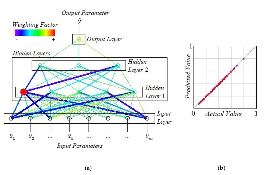
Developer”® software. The architecture of the ANN is shown in Figure 1 a.
In particular, in this case, 2 hidden neural layers are selected, the first of which contains 5 neurons,
and the second—3 neurons.
To train an artificial neural network with an array of normalized experimental data, the following
settings are selected: learning rate—0.01; momentum coefficient—0.1; transfer function—hyperbolic
tangent; the maximum number of training cycles—1 × 10⁶ ; target error—1 × 10⁻⁵ ; initialization
method of the threshold—random; initialization method of weighting factor—random; analysis update
interval—500 cycles.
As a result of training, the following convergence parameters are obtained: the sum of error—1.6
× 10 ; the average error per output per dataset—1.6 × 10⁻⁵ . Thus, the training accuracy of an artificial
−3
neural network is relatively high.
It should be noted that the following characteristics confirm the high accuracy of estimating
the value of the cutting force for an arbitrary set of input parameters using artificial intelligence:
regression coefficient—0.9994; slope—0.9993; y-intercept—0.0007. It confirms the validity of theMaterials 2020, 13, 5357 7 of 12
generated regression model. Visualization of the regression procedure’s convergence process resulting
from training an artificial neural network is shown in Figure 1b.
Figure 1. Artificial neural network architecture (a) and convergence of the regression procedure (b).
4.2. Multi-Parameter Quasi-Linear Regression Procedure
Despite the high accuracy of using artificial intelligence tools to determine the cutting force’s
dependence on the array of input parameters, it does not directly establish the corresponding
functional dependence. However, this problem can be solved by using a multi-parameter quasi-linear
regression procedure.
Thus, according to the generally accepted approach in mechanical engineering, justified in this
case by formula (1), any estimated value of y (for example, the cutting force) can be determined from
an array of input parameters xk using the following dependence:
m
β
Y
y=α xk k , (5)
k =1
which is a generalization of formula (1).
Since this relation is nonlinear, evaluation of its parameters α, βk is performed by logarithm; as a
result, formula (5) allows the obtaining of the corresponding quasi-linear model:
m
X
ȳ = ᾱ + βk x̄k , (6)
k =1
where the following symbols are introduced:
ȳ = lny; ᾱ = lnα; x̄k = lnxk . (7)
The parameters ᾱ, x̄k are evaluated by minimizing the target function of the total square
deviation [42]: n
m
2
X X
hii
R(ᾱ, {β̄}) = ᾱ + x̄k β̄k → min,
(8)
i=1 k =1
where β̄ —column vector of estimated indices of power βk ; x̄
k
—the logarithm of the value of the
k-th input parameter within the i-th experiment.Materials 2020, 13, 5357 8 of 12
The condition of a minimum of the target function R is the system of equations [43]
∂R
∂ᾱ = 0;
(9)
∂∂R = 0,
{β̄}
which, considering formula (8), takes the following expanded form:
!
n m
hii
ᾱ β̄
P P
+ x̄ = 0;
k k
i=1 k =1 (10)
!
n m
x̄hii β̄ x̄hii = 0,
P
ᾱ +
P
k k j
i=1 k =1
where j—the number of input parameter (j = 1, 2, . . . , m).
The last system of (m + 1) linear algebraic equations concerning parameters ᾱ, β̄k (k = 1, 2, . . . , m)
can be written in the following matrix form:
[C]{X} = {Y}, (11)
where [C], {X}, {F} are the stiffness matrix, the column vector of external influence, and the column
vector of the required parameters, respectively ᾱ, β̄k :
n | {S}T
ᾱ
( ) ( )
Y0
[C] = −− | −− ; {X} = ; {F} = , (12)
{B} {Y}
{S} | [D]
which in their structure contain the element Y0 , as well as the submatrix [D] and the column sub-vectors
{S} and {Y}, whose elements are defined by the following formulas:
n
X n
X n
X n
X
Y0 = ȳhii ; Yk = ȳhii x̄khii ; Sk = x̄hii
k
; D j,k = x̄hii
j k
x̄hii . (13)
i=1 i=1 i=1 i=1
Using the inverse matrix method allows the setting of the column vectors of the values of the
required parameters [44]:
−1
{X} = [C] {Y}. (14)
In this case, the total error of estimating the cutting force is determined by the formula:
v
m
t !2 X !2
1 ∂y ∂y
δPz = α δα + βk δ , (15)
Pz ∂α ∂βk βk
k =1
which considers expression (5) and, after identical transformations, takes the following form:
v
m
t
X
δPz = δ2α + (βk lnxk )2 δ2βk . (16)
k =1
For the array of experimental data shown in Table 2, the values of the required parameters
determined by the implementation of a multi-parameter quasi-linear regression procedure are obtained.
Therefore, for the total number of experiments n = 3 × 10⁴ , the calculation results, including the
estimation procedure’s errors, are summarized in Table 3.
Table 3. Estimation results of formula parameters (5).
Parameter α β1 β1 β1 β1 β1 β1 β1 β1
Predicted value 2.315 0.337 0.256 0.932 −0.051 −0.072 −0.072 −0.025 0.985
Actual value 2.254 0.342 0.258 0.945 −0.051 −0.072 −0.072 −0.026 1.000
Relative error, % 2.7 1.4 0.9 1.4 0.8 1.2 1.5 2.0 1.5
Negative values of the indices of power β4 , β5 , β6 , β6 confirm the inversely proportional dependence
of the cutting force Pz on the parameters Z, S, Spr , tpr in formula (1).Materials 2020, 13, 5357 9 of 12
A relatively small measurement error confirms the reliability of the results obtained. Thus,
the relative error in estimating the cutting force of coefficient α is 2.7%. The relative error in estimating
the indices of power βk is in the range of 0.8–1.5%. As a result, the total relative error in determining
the cutting force does not exceed 5.0%.
The input data have been varied in a range of 3% according to the uniform probability distribution
law to study the effect of varying parameters on the evaluated data disturbances. As a result,
the evaluated parameters’ average disturbances are in a range of 0.6–1.9%. Notably, the grinding
width B and the infeed speed Vp significantly impact the evaluated data (on average, 1.9% and
1.6%, respectively).
Finally, in production conditions, the proposed method allows the rapid and accurate assessment of
the influence of the workpiece’s parameters, tool, and the machine on the power characteristics’ values
for the cutting process. Its implementation requires experimental and statistical values of all necessary
parameters and software for electronic data processing and the calculation process’s automation.
5. Conclusions
Thus, in the presented research, a method was developed to calculate and predict indicators
that affect the cutting-force components during grinding to improve crankshaft machining efficiency.
Simultaneously, accurate and fast calculation of cutting-force values depending on the production
conditions makes it possible to adaptively control the crankpin grinding cycle’s parameters and ensure
the machining intensification.
The developed approach is based on creating a comprehensive scientific and methodological
approach for determining the quantitative values of parameters that determine the cutting force. As a
result, a method for conducting a virtual experiment to determine the cutting force depending on the
array of defining parameters was created. Moreover, artificial intelligence tools and multi-parameter
quasi-linear regression analysis made it possible to identify these parameters. A special feature of
the proposed approach lies in the possibility of considering the accuracy of determining unknown
coefficients of the regression model and controlling the total error in estimating the cutting force.
The reliability of the proposed approach of using artificial neural networks is confirmed by the
high value of Pearson’s product-moment correlation coefficient, which is equal to 0.9994. In general,
the reliability of the proposed mathematical model for determining the cutting force using regression
analysis is confirmed by the fact that for a given set of experimental data, the relative error in estimating
parameters that affect the cutting force does not exceed 1.5%. As a result, the total relative error in
determining the cutting force does not exceed 5.0%.
Finally, the developed scientific and methodological approach can be applied in a wide range
of further research fields. In particular, for correctly formed sets of experimental data, the suggested
algorithm of complex application of artificial intelligence tools and quasi-linear regression analysis
can be used not only for evaluating the components of cutting forces of turning, milling, drilling, etc.
but also for assessing the efficiency of technological processes in machines and apparatus.
Author Contributions: Conceptualization, I.P., I.K., and V.I.; methodology, M.S., A.K. and Y.B.; software, J.T. and
Y.B.; validation, I.P., A.K., and M.S.; formal analysis, I.K. and V.I.; investigation, J.T.; resources, Y.B. and A.K.;
data curation, Y.B.; writing—original draft preparation, I.P. and I.K.; writing—review and editing, M.S. and J.T.;
visualization, Y.B.; supervision, V.I. and I.K.; project administration, V.I.; funding acquisition, M.S. All authors
have read and agreed to the published version of the manuscript.
Funding: This research and APC was funded by APVV, grant number APVV-17-0310 “Implementation of the 4th
Industrial Revolution Principles in the Production of Tyre Components”.
Conflicts of Interest: The authors declare no conflict of interest.
References
1. Ivanov, V.; Dehtiarov, I.; Pavlenko, I.; Kosov, I.; Kosov, M. Technology for complex parts machining in
multiproduct manufacturing. Manag. Prod. Eng. Rev. 2019, 10, 25–36. [CrossRef]Materials 2020, 13, 5357 10 of 12
2. Karpus, V.; Ivanov, V.; Dehtiarov, I.; Zajac, J.; Kurichkina, V. Technological assurance of complex parts
manufacturing. In Advances in Design, Simulation and Manufacturing: DSMIE-2018; Lecture Notes in Mechanical
Engineering; Ivanov, V., Rong, Y., Trojanowska, J., Venus, J., Liaposhchenko, O., Zajac, J., Pavlenko, I., Edl, M.,
Perakovic, D., Eds.; Springer: Cham, Switzerland, 2019; pp. 51–61. [CrossRef]
3. Denysenko, Y.; Dynnyk, O.; Yashyna, T.; Malovana, N.; Zaloga, V. Implementation of CALS-Technologies in
quality management of product life cycle processes. In Advances in Design, Simulation and Manufacturing:
DSMIE-2018; Lecture Notes in Mechanical Engineering; Ivanov, V., Rong, Y., Trojanowska, J., Venus, J.,
Liaposhchenko, O., Zajac, J., Pavlenko, I., Edl, M., Perakovic, D., Eds.; Springer: Cham, Switzerland, 2019;
pp. 3–12. [CrossRef]
4. Dynnyk, O.; Denysenko, Y.; Zaloga, V.; Ivchenko, O.; Yashyna, T. Information support for the quality
management system assessment of engineering enterprises. In Advances in Design, Simulation and
Manufacturing II: DSMIE-2019; Lecture Notes in Mechanical Engineering; Ivanov, V., Trojanowska, J.,
Machado, J., Liaposhchenko, O., Zajac, J., Pavlenko, I., Edl, M., Perakovic, D., Eds.; Springer: Cham,
Switzerland, 2020; pp. 65–74. [CrossRef]
5. Yarovyi, Y.; Yarova, I. Energy criterion for metal machining methods. In Advances in Design, Simulation
and Manufacturing II: DSMIE-2019; Lecture Notes in Mechanical Engineering; Ivanov, V., Trojanowska, J.,
Machado, J., Liaposhchenko, O., Zajac, J., Pavlenko, I., Edl, M., Perakovic, D., Eds.; Springer: Cham,
Switzerland, 2020; pp. 378–387. [CrossRef]
6. Fesenko, A.; Basova, Y.; Ivanov, V.; Ivanova, M.; Yevsiukova, F.; Gasanov, M. Increasing of equipment
efficiency by intensification of technological processes. Period. Polytech. Mech. Eng. 2019, 63, 67–73. [CrossRef]
7. Krol, O.; Sokolov, V. Development of models and research into tooling for machining centers. East. Eur. J.
Enterp. Technol. 2018, 3, 12–22. [CrossRef]
8. Sokolov, V.; Krol, O.; Baturin, Y. Dynamics research and automatic control of technological equipment
with electrohydraulic drive. In Proceedings of the IEEE International Russian Automation Conference,
RusAutoCon 2019, Sochi, Russia, 8–14 September 2019; pp. 1–6. [CrossRef]
9. Basova, Y.; Nutsubidze, K.; Ivanova, M.; Slipchenko, S.; Kotliar, A. Design and numerical simulation of the
new design of the gripper for manipulating of the rotational parts. Diagnostyka 2018, 19, 11–18. [CrossRef]
10. Karpus, V.E.; Ivanov, V.A. Locating accuracy of shafts in V-blocks. Russ. Eng. Res. 2012, 32, 144–150. [CrossRef]
11. Denkena, B.; Gümmer, O. Active tailstock for precise alignment of precision forged crankshafts during
grinding. Procedia CIRP 2013, 12, 121–126. [CrossRef]
12. Dražumerič, R.; Roininen, R.; Badger, J.; Krajnik, P. Temperature-based method for determination of feed
increments in crankshaft grinding. J. Mater. Process. Technol. 2018, 259, 228–234. [CrossRef]
13. Aliakbari, K. Failure analysis of four-cylinder diesel engine crankshaft. J. Braz. Soc. Mech. Sci. Eng. 2019, 41.
[CrossRef]
14. Xu, X.L.; Yu, Z.W. Failure analysis of a truck diesel engine crankshaft. Eng. Fail. Anal. 2018, 92, 84–94. [CrossRef]
15. Belkhode, P.N. Optimum choice of the front suspension of an automobile. J. Eng. Sci. 2019, 6, E21–E24.
[CrossRef]
16. Citti, P.; Giorgetti, A.; Millefanti, U. Current challenges in material choice for high-performance engine
crankshaft. Procedia Structural Integrity 2018, 8, 486–500. [CrossRef]
17. Kostyuk, G. Prediction of the microhardness characteristics, the removable material volume for the durability
period, cutting tools durability and processing productivity depending on the grain size of the coating
or cutting tool base material. In Advances in Manufacturing II: MANUFACTURING 2019; Lecture Notes in
Mechanical Engineering; Gapinski, B., Szostak, M., Ivanov, V., Eds.; Springer: Cham, Switzerland, 2019;
Volume 4, pp. 300–316. [CrossRef]
18. Kostyuk, G.; Nechyporuk, M.; Kostyk, K. Determination of technological parameters for obtaining
nanostructures under pulse laser radiation on steel of drone engine parts. In Proceedings of the 10th
International Conference on Dependable Systems, Services and Technologies, DESSERT 2019, Leeds, UK,
5–7 June 2019; pp. 208–212. [CrossRef]
19. Martsynkovskyy, V.; Tarelnyk, V.; Konoplianchenko, I.; Gaponova, O.; Dumanchuk, M. Technology support
for protecting contacting surfaces of half-coupling—Shaft press joints against fretting wear. In Advances in
Design, Simulation and Manufacturing II: DSMIE-2019; Lecture Notes in Mechanical Engineering; Ivanov, V.,
Trojanowska, J., Machado, J., Liaposhchenko, O., Zajac, J., Pavlenko, I., Edl, M., Perakovic, D., Eds.; Springer:
Cham, Switzerland, 2020; pp. 216–225. [CrossRef]Materials 2020, 13, 5357 11 of 12
20. Tarelnyk, V.; Konoplianchenko, I.; Tarelnyk, N.; Kozachenko, A. Modeling technological parameters for
producing combined electrospark deposition coatings. In Proceedings of the International Conference on
Actual Problems of Engineering Mechanics, APEM 2019, Odessa, Ukraine, 20–24 May 2019; Surianinov, M.,
Ed.; Trans Tech Publications Ltd.: Baech, Switzerland, 2019; pp. 131–142. [CrossRef]
21. Da Silva, S.P.; Da Silva, E.J.; Coelho, R.T.; Rossi, M.A. Finding dimensional stability considering deflection
effects in cylindrical plunge grinding. J. Braz. Soc. Mech. Sci. Eng. 2019, 41, 555. [CrossRef]
22. Stepanov, M.; Ivanova, L.; Litovchenko, P.; Ivanova, M.; Basova, Y. Model of thermal state of the system of
application of coolant in grinding machine. In Advances in Design, Simulation and Manufacturing: DSMIE-2018;
Lecture Notes in Mechanical Engineering; Ivanov, V., Rong, Y., Trojanowska, J., Venus, J., Liaposhchenko, O.,
Zajac, J., Pavlenko, I., Edl, M., Perakovic, D., Eds.; Springer: Cham, Switzerland, 2019; pp. 156–165. [CrossRef]
23. Patel, A.; Bauer, R.J.; Warkentin, A. Investigation of the effect of speed ratio on workpiece surface topography
and grinding power in cylindrical plunge grinding using grooved and non-grooved grinding wheels. Int. J.
Adv. Manuf. Technol. 2019, 105, 2977–2987. [CrossRef]
24. Lezanski, P. A data-driven predictive model of the grinding wheel wear using the neural network approach.
J. Mach. Eng. 2017, 17, 69–82. [CrossRef]
25. Shapovalova, M.; Vodka, O. Image microstructure estimation algorithm of heterogeneous materials for
identification their chemical composition. In Proceedings of the 2nd IEEE Ukraine Conference on Electrical
and Computer Engineering, UKRCON 2019, Lviv, Ukraine, 2–6 July 2019. [CrossRef]
26. Lipiński, D.; Kacalak, W.; Bałasz, B. Optimization of sequential grinding process in a fuzzy environment
using genetic algorithms. J. Braz. Soc. Mech. Sci. Eng. 2019, 41, 96. [CrossRef]
27. Boaron, A.; Weingaertner, W.L. Dynamic in-process characterization method based on acoustic emission for
topographic assessment of conventional grinding wheels. Wear 2018, 406, 218–229. [CrossRef]
28. Botcha, B.; Rajagopal, V.; Bukkapatnam, S.T. Process-machine interactions and a multi-sensor fusion approach to
predict surface roughness in cylindrical plunge grinding process. Procedia Manuf. 2018, 26, 700–711. [CrossRef]
29. Steffan, M.; Haas, F.; Pierer, A.; Gentzen, J. Adaptive grinding process-prevention of thermal damage using
OPC-UA technique and in situ metrology. J. Manuf. Sci. Eng. Trans. ASME 2017, 139. [CrossRef]
30. Bordin, F.M.; Weingaertner, W.L. Steel subsurface damage on plunge cylindrical grinding with sol-gel
aluminum oxide grinding wheels. Int. J. Adv. Manuf. Technol. 2019, 105, 2907–2917. [CrossRef]
31. Kotliar, A.; Basova, Y.; Ivanova, M.; Gasanov, M.; Sazhniev, I. Technological assurance of machining accuracy
of crankshaft. In Advances in Manufacturing II: MANUFACTURING 2019; Lecture Notes in Mechanical
Engineering; Diering, M., Wieczorowski, M., Brown, C., Eds.; Springer: Cham, Switzerland, 2019; Volume 2,
pp. 37–51. [CrossRef]
32. Kotliar, A.; Gasanov, M.; Basova, Y.; Panamariova, O.; Gubskyi, S. Ensuring the reliability and performance
criterias of crankshafts. Diagnostyka 2019, 20, 23–32. [CrossRef]
33. Kundrák, J.; Fedorenko, D.O.; Fedorovich, V.A.; Fedorenko, E.Y.; Ostroverkh, E.V. Porous diamond grinding
wheels on ceramic binders: Design and manufacturing. Manuf. Technol. 2019, 19, 446–454. [CrossRef]
34. Sokhan’, S.V.; Maystrenko, A.L.; Kulich, V.H.; Sorochenko, V.H.; Voznyy, V.V.; Gamaniuk, M.P.; Zubaniev, Y.M.
Diamond grinding the ceramic balls from silicon carbide. J. Eng. Sci. 2018, 5, A12–A20. [CrossRef]
35. Kundrák, J.; Mamalis, A.G.; Fedorovich, V.; Pyzhov, I.; Kryukova, N. Evaluation of the characteristics of
diamond grinding wheels at their production and operation stages. Int. J. Adv. Manuf. Technol. 2018, 94,
1131–1137. [CrossRef]
36. Mamalis, A.G.; Grabchenko, A.I.; Mitsyk, A.V.; Fedorovich, V.A.; Kundrak, J. Mathematical simulation
of motion of working medium at finishing-grinding treatment in the oscillating reservoir. Int. J. Adv.
Manuf. Technol. 2014, 70, 263–276. [CrossRef]
37. Maier, M.; Rupenyan, A.; Bobst, C.; Wegener, K. Self-optimizing grinding machines using Gaussian process
models and constrained Bayesian optimization. Int. J. Adv. Manuf. Technol. 2020, 108, 539–552. [CrossRef]
38. Hernández-Becerro, P.; Purtschert, J.; Konvicka, J.; Buesser, C.; Schranz, D.; Mayr, J.; Wegener, K.
Reduced-order model of the environmental variation error of a precision five-axis machine tool. J. Manuf.
Sci. Eng. Trans. ASME 2021, 143, 021005. [CrossRef]
39. Pavlenko, I.V.; Simonovskiy, V.I.; Demianenko, M.M. Dynamic analysis of centrifugal machines rotors
supported on ball bearings by combined application of 3D and beam finite element models. In Proceedings
of the 15th International Scientific and Engineering Conference Hermetic Sealing, Vibration Reliability
and Ecological Safety of Pump and Compressor Machinery, HERVICON+PUMPS 2017, Sumy, Ukraine,
5–8 September 2017; Institute of Physics Publishing: Bristol, UK, 2017. [CrossRef]Materials 2020, 13, 5357 12 of 12
40. Pavlenko, I.; Ivanov, V.; Kuric, I.; Gusak, O.; Liaposhchenko, O. Ensuring vibration reliability of turbopump
units using artificial neural networks. In Advances in Manufacturing II: MANUFACTURING 2019; Lecture
Notes in Mechanical Engineering; Trojanowska, J., Ciszak, O., Machado, J., Pavlenko, I., Eds.; Springer:
Cham, Switzerland, 2019; Volume 1, pp. 166–175. [CrossRef]
41. Pavlenko, I.; Trojanowska, J.; Ivanov, V.; Liaposhchenko, O. Parameter identification of hydro-mechanical
processes using artificial intelligence systems. Int. J. Mechatron. Appl. Mech. 2019, 2019, 19–26.
42. Sacks, J.; Welch, W.J.; Mitchell, T.J.; Wynn, H.P. Design and analysis of computer experiments. Stat. Sci. 1989,
4, 409–423. [CrossRef]
43. Ye, Y.; Wang, Z.; Zhang, X. An optimal pointwise weighted ensemble of surrogates based on minimization of
local mean square error. Struct. Multidiscip. Optim. 2020, 62, 529–542. [CrossRef]
44. Filelis-Papadopoulos, C.K.; Gravvanis, G.A. Generic approximate sparse inverse matrix techniques. Int. J.
Comput. Methods 2014, 11, 1350084. [CrossRef]
Publisher’s Note: MDPI stays neutral with regard to jurisdictional claims in published maps and institutional
affiliations.
© 2020 by the authors. Licensee MDPI, Basel, Switzerland. This article is an open access
article distributed under the terms and conditions of the Creative Commons Attribution
(CC BY) license (http://creativecommons.org/licenses/by/4.0/).You can also read