COCONET: A COLLABORATIVE CONVOLUTIONAL NETWORK
←
→
Page content transcription
If your browser does not render page correctly, please read the page content below
CoCoNet: A Collaborative Convolutional Network
                                                 Tapabrata Chakraborti1,2 , Brendan McCane1 , Steven Mills1 , and Umapada Pal2
                                                                  1
                                                                      Dept. of Computer Science, University of Otago, NZ
                                                                        2
                                                                          CVPR Unit, Indian Statistical Institute, India

                                                                                         November 11, 2020

                                                                                                 Abstract
                                                   We present an end-to-end deep network for fine-grained visual categorization called Collaborative Convolu-
arXiv:1901.09886v4 [cs.CV] 9 Nov 2020

                                              tional Network (CoCoNet). The network uses a collaborative layer after the convolutional layers to represent an
                                              image as an optimal weighted collaboration of features learned from training samples as a whole rather than one
                                              at a time. This gives CoCoNet more power to encode the fine-grained nature of the data with limited samples. We
                                              perform a detailed study of the performance with 1-stage and 2-stage transfer learning. The ablation study shows
                                              that the proposed method outperforms its constituent parts consistently. CoCoNet also outperforms few state-
                                              of-the-art competing methods. Experiments have been performed on the fine-grained bird species classification
                                              problem as a representative example, but the method may be applied to other similar tasks. We also introduce
                                              a new public dataset for fine-grained species recognition, that of Indian endemic birds and have reported initial
                                              results on it.

                                        1    Introduction
                                        Deep convolutional networks have proven to be effective in classifying base image categories with sufficient
                                        generalization when trained with a large dataset. However, many real life applications of significance [1] may
                                        be characterized by fine-grained classes and limited availability of data, like endangered species recognition or
                                        analysis of biomedical images of a rare pathology. In such specialized problems, it is challenging to effectively
                                        train deep networks that are, by nature, data hungry. A case in point is that of fine-grained endangered species
                                        recognition [2], where besides scarcity of training data, there are further bottlenecks like subtle inter-class object
                                        differences compared to significant randomized background variation both between and within classes. This is
                                        illustrated in Fig. 1. Added to these, is the presence of the “long tail” problem [3], that is, significant imbalance
                                        in samples per class (the frequency distribution of samples per class has long tail).
                                        Transfer learning is a popular approach to train on small fine-grained image datasets with limited samples [4].
                                        The ConvNet architecture is trained first on a large benchmark image dataset (e.g. ImageNet) for the task of
                                        base object recognition. The network is then fine-tuned on the smaller target dataset for fine-grained recognition.
                                        Since the target dataset is small, there is an increased chance of overtraining. On the other hand, if the dataset
                                        has fine-grained objects with varying backgrounds, this can cause difficulty in training convergence. This makes
                                        the optimal training of the dataset challenging [3]. In case of small datasets with imbalanced classes, the problem
                                        is compounded by the probability of training bias in favour of larger classes. A few specialized deep learning
                                        methods have been proposed in recent times to cater to these issues, like low-shot/zero-shot learning [5] for small
                                        datasets and multi-staged transfer learning [4] for fine-grained classes. In spite of these advances, deep learning
                                        of small fine-grained datasets remains one of the open popular challenges of machine vision [6][7].
                                        Recently, Chakraborti et al. [8] demonstrated that collaborative filters can effectively represent and classify small
                                        fine-grained datasets. Collaborative filters have been the method of choice for recommender systems [19] and
                                        have recently also been used in vision systems like face recognition [9]. Cai et al. [10] have recently shown
                                        that some modern versions of Collaborative Representation Classifiers (CRC) give better performance with CNN
                                        learned features from a pre-trained ConvNet compared to softmax based classification layer [10].
                                        The intuition why collaborative filtering works well to represent fine-grained data is as follows. Collaborative
                                        representation classifiers (CRC) [9] represent the test image as an optimal weighted average of all training images

                                                                                                     1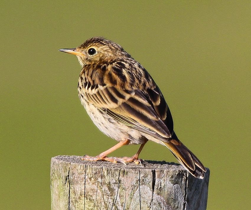
across all classes. The predicted label is the class having least residual. This inter-class collaboration for opti-
mal feature representation is distinct from the traditional purely discriminative approach. Thus the collaborative
scheme not only takes advantages of differences between object categories but also exploits the similarities of fine-
grained data. Other advantages are that CRC is analytic since it has a closed form solution and is time efficient
since it does not need iterative or heuristic optimization. It is also a general feature representation-classification
scheme and thus most popular feature descriptors and ensembles thereof are compatible with it. The present work
advances the state-of-the-art by encoding the collaborative loss function into a deep CNN model. The contribu-
tions of this paper are two-fold.
1. Collaborative ConvNet (CoCoNet): The proposed method fine-tunes a pre-trained deep network through a
collaborative representation classifier in an end-to-end fashion. This establishes a protocol for multi-stage transfer
learning of fine-grained data with limited samples. We test it for fine-grained bird species recognition as an
example, but the same may be applied to other similar tasks.
2. Indian Birds dataset: We introduce IndBirds, a new fine-grained image benchmark of Indian endemic birds.
It currently has 800 images of 8 classes (100 images per class). All experiments have been repeated on the new
dataset and results are presented.
2 Collaborative Convolutional Network
We first present a brief description of the original collaborative representation classifier (CRC) [9] and then the
proposed Collaborative ConvNet (CoCoNet).
2.1 Collaborative Representation Classifier (CRC)
Consider a training dataset with images in the feature space as X = [X1 , . . . , Xc ] ∈ d×n where n is the total
number of samples over c classes and d is the feature dimension per sample. Thus Xi ∈ d×ni is the feature space
representation of class i with ni samples such that ci=1 ni = n.
P
The CRC model reconstructs a test image in the feature space ~y ∈ d as an optimal collaboration of all training
samples, while at the same time limiting the size of the reconstruction parameters, using the l2 regularisation term
λ.
The CRC cost function is given by:
J(α, λ) = k~y − Xαk22 + λkαk22 (1)
where α̂ = [α̂1 , . . . , α̂c ] ∈ N | α̂i ∈ ni is the reconstruction matrix corresponding to class i.
A least-squares derivation yields the optimal solution for α as:
α̂ = (X T X + λI)−1 X T ~y (2)
The representation residual of class i for test sample ~y can be calculated as:
k~y − Xi α̂i k22
ri (~y) = ∀i ∈ 1, . . . , c (3)
kα̂i k22
The final class of test sample ~y is thus given by
C(~y) = arg min ri (~y) (4)
i
The optimal value of λ is determined using gradient descent.
2.2 Collaborative ConvNet (CoCoNet)
CoCoNet gives a collaborative cost which is back propagated through an end-to-end model. The training set is
divided into two sections p1 and p2, having m and n images respectively randomly selected with equal represen-
tation across classes.
2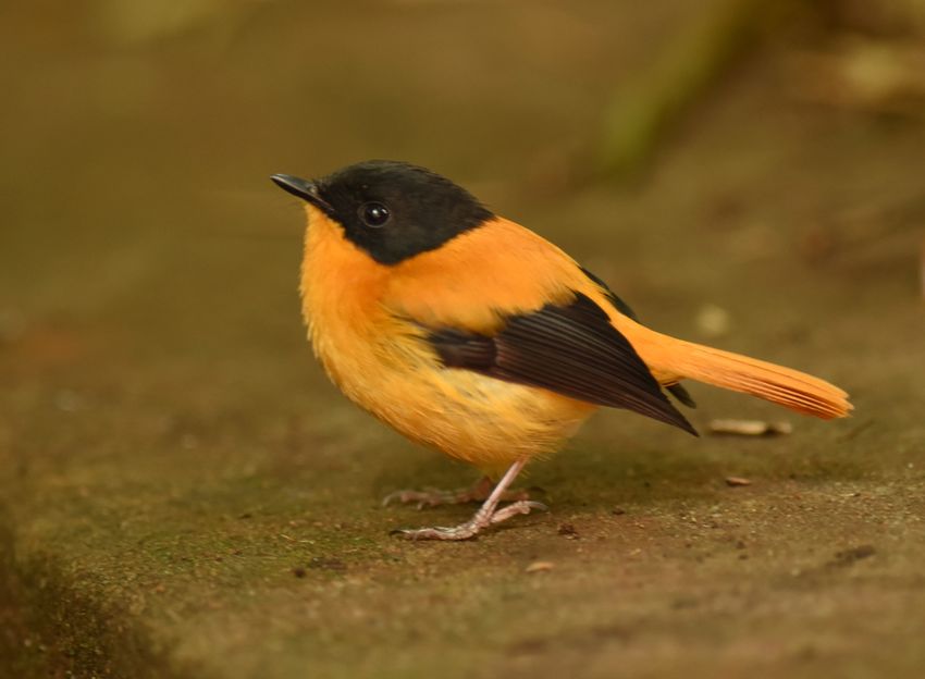
Figure 1: Architecture of the proposed Collaborative ConvNet (CoCoNet). Training samples are divided into two
partitions which collaborate to represent fine-grained patterns. The collaborative cost function generates the error
that optimizes its own parameters as well as fine-tune the network weights in an end-to-end manner.
Let x be the d × 1 feature vector of one image in p1, such that the feature matrix for p1 is X of dimension d × m.
Let y be the d × 1 feature vector of one image in p2, such that the feature matrix for p2 is Y of dimension d × n.
The collaborative cost function is given by:
P (A, W, X) = k(Y − XA)Wk22 + λkAk22 + γkWk22 (5)
The collaborative reconstruction matrix A is thus of dimension m × n. The goal is to find an optimal feature
representation of each sample in p2 with respect to the “training” images in p1 via a representation vector ~ai ∈ A.
The weight matrix W is used to compensate for imbalance of classes and each of its elements is initialised with a
weight proportional to the size of the class to which the corresponding feature vector in Y belongs. W counteracts
the imbalance in classes as a penalty term for larger classes by increasing the cost. W is of dimension n × 1.
After finding the initial optimal A through least squares, it is then updated along with the weight matrix W through
partial derivatives. The gradient of the feature matrix X is then used to update the CNN weights through back-
propagation as presented in Algorithm 1.
Least squares minimization gives the initial optimal value of A as:
h i−1
 = X T XW T W + λI X T YWW T (6)
Fix A, X , update W:
∂P
= −(Y − XA)T (Y − XA)W + γW (7)
∂W
Fix W, X , update A:
∂P
= −X T (Y − XA)WW T + λA (8)
∂A
Fix W, A , update X:
∂P
= −(Y − XA)WW T AT (9)
∂X
Once all the partial derivatives are obtained, CNN weights are updated by standard back-propagation of gradients
for each batch in P1 and P2. The training iterations are continued until the error stabilizes. A schematic of the
CoCoNet architecture is presented in Fig. 1.
3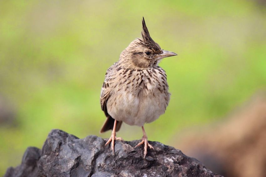
Algorithm 1: Training with CoCoNet
 1   Initiate weight matrix W proportional to class size ;
 2   Split the training set into two parts P1 and P2 ;
 3   Extract feature matrix X of P1 through CNN section. ;
 4   Find initial optimal reconstruction matrix A by eqn. 6. ;
 5   for each sample in P2 do

 6       Fix A, X , update W by eqn. 7 ;

 7       Fix W, X , update A by eqn. 8 ;
 8       for each sample in P1 do
 9           Back-propagate to update weights using eqn. 9 ;
10       end
11   end

     2.3    Reducing computation cost through SVD.
     The optimal representation weight matrix  from eqn 6. has the term (X T XW T W + λI)−1 , where X is of dimen-
     sion d × m. Here d is the dimension of the descriptor and m is the total number of data points in the partition
     P1 of training data. This poses the problem of high computation cost for large datasets (m is large). So we use
     singular value decomposition (SVD) to reduce the matrix inverse computation to dimension d × d, so as to make it
     independent of dataset size. This is a crucial modification needed for applications like image retrieval from large
     unlabeled or weakly labeled image repositories.

     If we take the singular value decomposition (SVD) of X T , we can factor X T X as:

                                     X T X = (US V T )T US V T = VS T U T US V T = V(S 2 )V T                       (10)

     Since S only has d non-zero singular values, we can truncate S T S and V to be smaller matrices. So V is N × d, S
     is d × d and V T is d × N. Also note that since W is of dimension n × 1, W T W comes out as a scalar value in eqn.
     6, which is absorbed in S to have Ŝ .
     Using the Woodbury matrix inverse identity [18], the inverse term becomes (V Ŝ 2 V T + λI)−1 which can be repre-
     sented as:
                              1    1            1               1     1         1
                                 + 2 V(Ŝ −1 + V T V)−1 V T = + 2 V(Ŝ −1 + I)−1 V T                              (11)
                              λ λ               λ               λ λ             λ

     Note that the inverse term (Ŝ −1 + λ1 I)−1 is only d × d, so it scales to many data points.

     2.4    Enhanced Learning by CoCoNet
     CoCoNet uses the collaborative cost function in an end-to-end manner. So we do not have the fully connected,
     energy loss function and softmax layers. The CNN extracts features and feeds it to the collaborative layer. The
     collaborative cost function estimates error, updates its own weights as well as feeds the error back to the CNN.
     The error and gradients are then back propagated through the CNN to update the weights. So CoCoNet is different
     from just cascading a CNN based feature learner with a collaborative filter, because the weights are not updated
     in latter in an end-to-end fashion. For the same dataset and same number of given samples, the collaborative
     filter represents all samples together as an augmented feature vector. Thus after the error is calculated, the error
     gradients are then back propagated. This collaborative representation is not just the augmented feature matrix with
     all samples, it is also optimised by the collaborative filter. This adds an additional level of optimisation besides
     the CNN learned features, weights and tuned parameters.

                                                                 4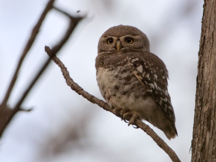
3 Experiments and Results
3.1 Datasets
Five benchmark image datasets are used in this work for pre-training and fine-tuning in total.
ImageNet [11] has about 1.4 million image categories and about 22k indexed sysnet as of 2017. It has been used
for pre-training the networks as base category classifiers. Then for transfer learning, the following bird species
recognition datasets have been used.
NABirds [12] is a fine-grained North American bird species recognition dataset developed by Cornell-UCSD-
CalTech collaboration and maintained by the Cornell Lab of Ornithology. It is continually updated and at the time
of use for this work had 555 classes and 48562 images. Due to the large number of images present in this dataset,
it may be used for training a deep network from scratch as well as for transfer learning.
CUB 200-2011 [13] dataset contains 11,788 images of 200 bird species. The main challenge of this dataset is con-
siderable variation and confounding features in background information compared to subtle inter-class differences
in birds.
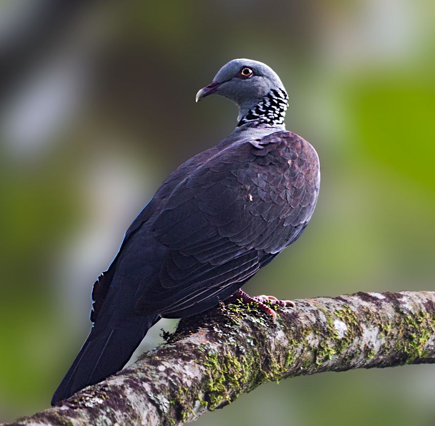
IndBirds is a new bird species recognition benchmark compiled as part of this work by the Indian Statistical
Institute and University of xxxx, NZ. The dataset contains images of 8 species of Indian endemic birds with
around 100 images per class, collected from web repositories of birders and citizen scientists. The dataset is
available for academic use from the lead author. Sample images of each class are presented in Fig. 2.
NZBirds [14] is a small benchmark dataset of fine-grained images of NZ endemic birds, many of which are
endangered. Currently it contains 600 images of 30 NZ birds and has been compiled by University of Otago
in collaboration with The National Museum of NZ (Te Papa), the Department of Conservation (DOC) and the
Ornithological Society of NZ (Birds NZ).
3.2 Competing Classifiers
We evaluate the performance of CoCoNet against popular recent methods both among collaborative representation
classifiers (CRC) and deep convolutional neural networks (CNN), besides testing against constituent components
in an ablation study. Among current CRC methods, we compare against the recent Probabilistic CRC (ProCRC)
[10]. Among recent deep CNN models, we choose the popular Bilinear CNN [20],[21] and the very recent NTS-
Net as the benchmark competitors [24].
Of course, there are a few more recent variants of ProCRC, like enhanced ProcCRC (EProCRC) [22], as well
as BCNN, like improved BCNN [23]. However, we have deliberately used the vanilla versions because the aim
is to establish a baselne evaluation in this work. For the same reason we also compare with the original CRC
formulation [9] with VGG19 by Simonyan et al. [16] as the CNN backbone.
Probabilistic CRC (ProCRC). Cai et al. [10] presented a probabilistic formulation (ProCRC) of the CRC
method. Each of these probabilities are modeled by Gaussian exponentials and the probability of test image y
belonging to a class k is expanded by chain rule using conditional probability. The final cost function for ProCRC
is formulated as maximisation of the joint probability of the test image belonging to each of the possible classes
as independent events. The final classification is performed by checking which class has the maximum likelihood.
K
γ X
J(α, λ, γ) = ky − Xαk22 + λkαk22 + kXα − Xk αk k22 (12)
K k=1
Bilinear CNN. Maji et al. introduced the BCNN architecture for fine-grained visual recognition [20],[21]. These
networks represent an image as a pooled outer product of features learned from two CNNs and encode localized
feature interactions that are translationally invariant. B-CNN is a type of orderless texture representations that can
be trained in an end-to-end manner.
5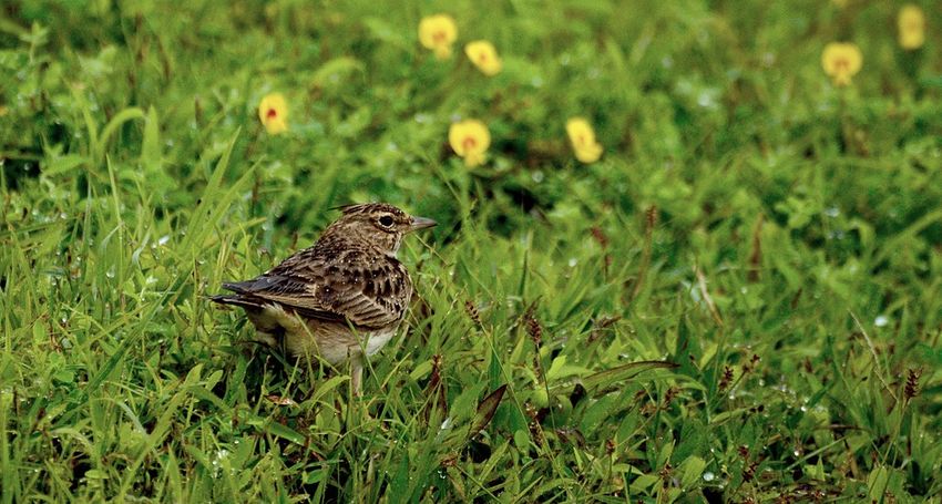
Nilgiri Wood Pigeon

                                             Nigiri Fly Catcher

                                           Malabar Grey Hornbill

                                                Nilgiri Pipit

                                               Forest Owlet

                                              Rufous Babbler

                                               Malabar Lark

                                        Black and Orange Flycatcher

                         Figure 2: New IndBirds dataset: 8 classes; 100 images each

SOTA methods. Besides the above, we also compare the performance of our method against several state-of-
the-art approaches reported on the benchmark CUB dataset in ICCV 2019. These are Cross-X Learning [25],
Deconstruction Construction Learning (DCL) [26], Trilinear Attention Sampling Network (TASN) [27], Selective
Spars Sampling (S3N) [28] and Mixture of Granularity-Specific Experts (MGE-CNN) [29]. We see that our
method compares favourably with these recent methods reported in results section.

                                                     6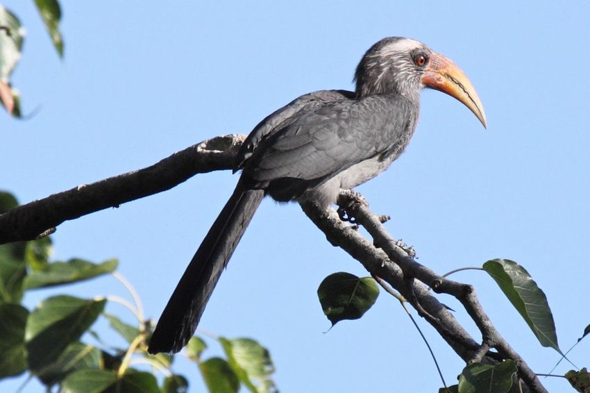
Table 1: CUB 200-2011 Test Accuracy (%)

                                              ImageNet         NABirds      ImageNet →
                                               → CUB           → CUB         NABirds→
                                               (1 stage)       (1 stage)      CUB
                                                                              (2 stage)

                           Vgg19              71.9 ± 5.5       74.1 ± 5.7    77.5 ± 5.9

                           Vgg19+CRC          76.2 ± 5.6       79.0 ± 5.5    80.2 ± 5.9

                           Vgg19+ProCRC 79.3 ± 5.4             82.5 ± 5.5    83.8 ± 5.8

                           CoCoNet3           83.6 ± 5.5       87.4 ± 5.6    89.1 ± 5.6

                           Bilinear-CNN       84.0 ± 5.3       85.7 ± 5.8    87.2 ± 5.5

                                        Table 2: IndBirds Test Accuracy (%)

                                              ImageNet         NABirds      ImageNet →
                                                   →               →        NABirds. →
                                              IndBirds         IndBirds      IndBirds (2
                                               (1 stage)       (1 stage)       stage)

                           Vgg19              76.2 ± 4.2       82.5 ± 4.7    84.8 ± 4.2

                           Vgg19+CRC          80.6 ± 4.4       86.3 ± 4.0    87.4 ± 4.4

                           Vgg19+ProCRC 84.0 ± 4.9             89.1 ± 4.1    91.0 ± 4.2

                           CoCoNet3           87.4 ± 4.3       92.9 ± 4.4    94.7 ± 4.5

                           Bilinear-CNN       85.1 ± 4.7       88.6 ± 4.2    91.5 ± 4.3

3.3    Experiments
We train each of the three target datasets (CUB, NZBirds, IndBirds) through a combination of one stage and two
stage transfer learning. For one stage transfer learning, two separate configurations have been used: 1) the network
is pre-trained for general object recognition on ImageNet and then fine-tuned on the target dataset; 2) the network
is pre-trained for bird recognition on the large north american bird dataset (NABirds) and then fine-tuned on the
target dataset. For two stage training, the network is trained successively on ImageNet, NABirds and then the
target dataset. Note that for pre-training, always the original architecture (VggNet) is used, CoCoNet only comes
into play during fine-tuning. During both pre-training and fine-tuning, we start with 0.001 learning rate, but shift to
0.0001 once there is no change in loss anymore, keeping the total number of iterations/epochs constant at 1000 and
using the Adam [17] optimiser. We investigate how the end-to-end formulation of CoCoNet fares in controlled
experiments with competing configurations. We perform the same experiments using the original architecture
(VggNet), then we observe change in accuracy with cascaded CNN+CRC and the end-to-end CoCoNet. We also
further tabulate the results with cascaded CNN+ProCRC as well as Bilinear CNN [23]. For each dataset, images
are resized to 128×128 and experiments are conducted with five-fold cross validation.

                                                           7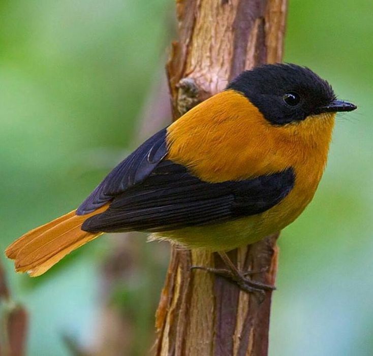
Table 3: NZBirds Test Accuracy (%)

                                             ImageNet         NABirds             ImageNet →
                                                  →               →                NABirds →
                                             NZBirds          NZBirds              NZBirds (2
                                              (1 stage)       (1 stage)              stage)

                           Vgg19             61.5 ± 5.0       63.7 ± 5.1           65.6 ± 5.7

                           Vgg19+CRC         63.9 ± 5.3       66.1 ± 5.5           68.7 ± 5.6

                           Vgg19+ProCRC 66.2 ± 5.5            71.3 ± 5.1           72.9 ± 5.8

                           CoCoNet3          71.8 ± 5.2       74.4 ± 5.2           77.2 ± 5.6

                           Bilinear-CNN      69.4 ± 5.6       71.8 ± 5.5           73.3 ± 5.0

          Cross-X [25]    DCL [26]     TASN [27]     S3N [28]     MGE-CNN [29]           CoCoNet   CoCoNet
                                                                                         1-stage   2-stage
               88.5          87.7         88.5         87.9                87.8          87.4      89.1

             Table 4: CoCoNet with 2 stage transfer learning against state-of-the-art on CUB dataset

3.4    Results and Analysis
Percentage classification accuracies along with standard deviation are presented in Table 1 (CUB), Table 2 (Ind-
Birds) and Table 3 (NZBirds). It may be readily observed from the tabulated results, that the proposed method
overall outperforms its competitors, including the probabilistic CRC (ProCRC), bilinear CNN (BCNN). This per-
formance is reflected across the three datasets and two stage transfer learning performs better than one stage for
all classifiers. We compare with i) just a direct VggNet with the standard Softmax classfier and ii) VggNet as pre-
trained feature extractor cascaded with a collaborative classifier (CRC) but not integrated. CoCoNet outperforms
both of them as well as VggNet cascaded with probabilistic CRC (ProCRC), which is a more recent collaborative
classifier. A qualitative example is presented in Fig. 3.

Statistical Analysis. We perform the Signed Binomial Test [30] to investigate the statistical significance of the
improvement in performance of CoCoNet vs. BCNN, since these have the closest performances. The null hy-
pothesis is that the two competitors are equally good, that is there is 50% chance of each beating the other on any
particular trial. For each of the three datasets (CUB, NZBirds and Indbirds), there are three transfer learning con-
figurations (two single stage and a double stage) and five-fold cross-validated results. Thus over the three datasets,
in total we have 45 experiments of CoCoNet vs. each of its competitors. Out of these CoCoNet outperformed
BCNN 33 times (that is 73.33% of the trials). The signed binomial test yields that given the assumption that both
methods are equally good, then the probability of CoCoNet outperforming BCNN in 73.33% of the trials is has
one -tail p-value of 0.0012 and 2-tail p-value of 0.0025. Considering a level of significance of α = 0.05, we have
to apply the Bonferroni adjustment. We have 3 transfer learning protocols and 3 datasets: hence 9 combinations
of experimental condition. So we divide the 5% level of significance by 9 to get adjusted α = 0.0055. Since the
p-values obtained in both cases is less than 0.0055, it may be concluded that the improvement in accuracy of the
proposed method is statistically significant.

SOTA Comparison. In Table 4, we compare the performance of our method directly against several state-of-
the-art methods from ICCV 2019 that reported results on the CUB dataset. These are Cross-X Learning [25],
Deconstruction Construction Learning (DCL) [26], Trilinear Attention Sampling Network (TASN) [27], Selective
Spars Sampling (S3N) [28] and Mixture of Granularity-Specific Experts (MGE-CNN) [29]. It can be noted that our
method outperforms them for 2-stage transfer learning and for 1-stage transfer learning, the results are comparable.

                                                          8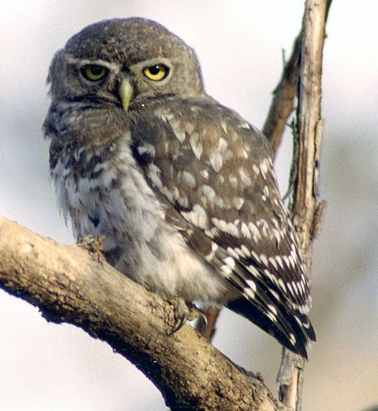
(a)                (b)                 (c)                (d)                (e)                 (f)

Figure 3: Classification and Misclassification Examples from the new IndBirds dataset: (a) Malabar Lark, (b)
Nilgiri Pipit, (c) Malabar Lark, misclassified as Nilgiri Pipit by both proposed CoCoNet and competitors, due
to obfuscation of the discriminating head crest. (d) Nilgiri Pipit with characteristic dark pattern on back (e)
Front-facing image of Nilgiri Pipit with back patterns not visible. Correctly classified by proposed CoCoNet but
misclassified by competitors as Rufous Babbler (f).

4    Conclusion
We present an end-to-end collaborative convolutional network (CoCoNet) architecture for fine-grained visual
recognition of bird species with limited samples. The new architecture adds a collaborative representation which
adds an additional level of optimization based on collaboration of images across classes, the information is then
back-propagated to update CNN weights in an end-to-end fashion. This collaborative representation exploits the
fine-grained nature of the data better with fewer training images. The proposed network is evaluated for the task
of fine-grained bird species recognition, but the method is general enough to perform other fine-grained classifica-
tion tasks like detection of rare pathology from medical images. The other major advantage is that most existing
CNN architectures can be easily restructured into the proposed configuration. We also present a new fine-grained
benchmark dataset with images of endemic Indian birds, and report results on it. Results show that the proposed
algorithm performs better than its constituent parts and several state-of-the-art competitors.

References
[1] Y. Chai. Advances in Fine-grained Visual Categorization. University of Oxford, 2015.
[2] E. Rodner, M. Simon, G. Brehm, S. Pietsch, J.-W.Wägele, and J. Denzler. Fine-grained Recognition Datasets
    for Biodiversity Analysis. In Proc. CVPR, 2015.
[3] G. V. Horn and P. Perona, “The Devil is in the Tails:               Fine-grained Classification in the Wild”,
    arXiv:1709.01450 [cs.CV], 2017.
[4] M. Simon and E. Rodner, “Neural Activation Constellations: Unsupervised Part Model Discovery with Con-
    volutional Networks”, In Proc. ICCV, 2015.
[5] A. Li, Z. Lu, L. Wang, T. Xiang, X. Li, J-R Wen, “Zero-Shot Fine-Grained Classification by Deep Feature
    Learning with Semantics”, arXiv:1707.00785 [cs.CV], 2017.
[6] J. Krause, T. Gebru, J. Deng, L.-J.Li,and F.-F. Li. Learning Features and Parts for Fine-Grained Recognition.
    In Proc. ICPR, 2014.
[7] J. Krause, H. Jin, J. Yang, and F.-F.Li. Fine-grained recognition without part annotations. In Proc. CVPR,
    2015.
[8] T. Chakraborti, B. McCane, S. Mills, and U. Pal, “A Generalised Formulation for Collaborative Representation
    of Image Patches (GP-CRC)”, In Proc. BMVC, 2017.
[9] L. Zhang, M. Yang, and X. Feng. Sparse representation or collaborative representation: Which helps face
    recognition? In Proc. ICCV, 2011.
[10] S. Cai, L. Zhang, W. Zuo, and X. Feng. A probabilistic collaborative representation based approach for
    pattern classification. CVPR, 2016.

                                                         9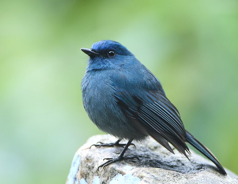
[11] O. Russakovsky, J. Deng, H. Su, J. Krause, S. Satheesh, S. Ma, Z. Huang, A. Karpathy, A. Khosla, M.
    Bernstein, A. C. Berg, and Li Fei-Fei, “ImageNet Large Scale Visual Recognition Challenge,” International
    Journal of Computer Vision, 2015.
[12] G. V. Horn, S. Branson, R. Farrell, S. Haber, J. Barry, P. Ipeirotis, P. Perona, S. J. Belongie, “Building a bird
    recognition app and large scale dataset with citizen scientists: The fine print in fine-grained dataset collection
    ”, In Proc. CVPR, 2015.
[13] C. Wah, S. Branson, P. Welinder, P. Perona, and S. Belongie. The caltech-ucsd birds-200-2011 dataset.
    http://www.vision.caltech.edu/visipedia/CUB-200-2011.html.
[14] T. Chakraborti, B. McCane, S. Mills, and U. Pal, “Collaborative representation based fine-grained species
    recognition”, In Proc. IVCNZ, 2016.
[15] A. Krizhevsky, I. Sutskever, G. E. Hinton, “ImageNet Classification with Deep Convolutional Neural Net-
    works”, In Proc. NIPS, 2012.
[16] K. Simonyan and A. Zisserman. Very deep convolutional networks for large-scale image recognition. In
    Proc. ICLR, 2014.
[17] D. P. Kingma and J. Ba, “Adam: A Method for Stochastic Optimization”, In Proc. ICLR, 2015.
[18] M. A. Woodbury, “Inverting modified matrices”, Memorandum report, vol. 42, no. 106, pp. 336, 1950.
[19] J. B. Schafer, D. Frankowski, J. Herlocker and S. Sen, “Collaborative Filtering Recommender Systems”, The
    Adaptive Web, Lecture Notes in Computer Science, Springer, vol. 4321, pp. 291-324, 2018.
[20] T-Y Lin, A. RoyChowdhury, and S. Maji, “Bilinear Convolutional Neural Networks for Fine-Grained Visual
    Recognition”, IEEE Trans. Pattern Anal. Mach. Intell., vol. 40, no. 6, pp. 1309-1322, 2018.
[21] T-Y Lin, A. RoyChowdhury, S. Maji, “Bilinear CNN Models for Fine-Grained Visual Recognition”, In Proc.
    ICCV, pp. 1449-1457, 2015.
[22] R. Lan and Y. Zhou, “An extended probabilistic collaborative represen-tation based classifier for image
    classification”, In Proc. IEEE Intl. Conf.on Multimedia and Expo (ICME), 2017.
[23] T-Y Lin, and S. Maji, “Improved Bilinear Pooling with CNNs”, In Proc. BMVC, 2017.
[24] Z. Yang, T Luo, D. Wang, Z. Hu, J. Gao, and L. Wang, “Learning to Navigate for Fine-grained Classifica-
    tion”, In Proc. ECCV, 2018.
[25] W. Luo, X. Yang, X. Mo, Y. Lu, L. S. Davis, J. Li, J. Yang, and S-N. Lim, “Cross-X Learning for Fine-
    Grained Visual Categorization”, In Proc. ICCV, 2019.
[26] Y. Chen, Y. Bai, W. Zhang, and T. Mei, “Destruction and Construction Learning for Fine-grained Image
    Recognition”, In Proc. CVPR, 2019.
[27] H. Zheng, J. Fu, Z-J. Zha, and J. Luo, “Looking for the Devil in the Details: Learning Trilinear Attention
    Sampling Network for Fine-grained Image Recognition”, In Proc. CVPR, 2019.
[28] Y. Ding, Y. Zhou, Y. Zhu, Q. Ye, and J. Jiao, “Selective Sparse Sampling for Fine-grained Image Recogni-
    tion”, In Proc. ICCV, 2019.
[29] L. Zhang, S. Huang, W. Liu, and D. Tao, “Learning a Mixture of Granularity-Specific Experts for Fine-
    Grained Categorization”, In Proc. ICCV, 2019.
[30] J. Demsar, “Statistical Comparisons of Classifiers over Multiple Data Sets”, Journal of Machine Learning
    Research, vol. 7, pp. 1-30, 2006.

                                                         10
You can also read