MRI Radiomics: Tumor Identification and Reverse Image Search Using Convolutional Neural Network - WWT
←
→
Page content transcription
If your browser does not render page correctly, please read the page content below
MRI Radiomics: Tumor
Identification and Reverse
Image Search Using
Convolutional Neural Network

FEBRUARY | 2021

Authors: Jim Winkelmann; Sai Pokkunuri;
Pulkit Bansal; Mohammad Faisal, NLN;
Henry Stoltenberg and William Wolfe

World Wide Technology
www.wwt.com
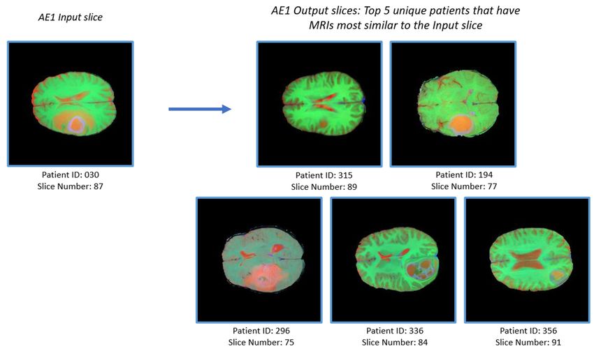
Table of Contents
Abstract. . . . . . . . . . . . . . . . . . . . . . . . . . . . . . . . . . . . . . . . . . . . . . . . . . . . . . . . . . . . . . . . . . . . . . . . . . . . . . . . . . . . . . . . . . . . . . . . . . . . . . . . 3

Business Justification. . . . . . . . . . . . . . . . . . . . . . . . . . . . . . . . . . . . . . . . . . . . . . . . . . . . . . . . . . . . . . . . . . . . . . . . . . . . . . . . . . . . . . . . . . . . 3

Experimental Setup and Methodology. . . . . . . . . . . . . . . . . . . . . . . . . . . . . . . . . . . . . . . . . . . . . . . . . . . . . . . . . . . . . . . . . . . . . . . . . . . . 5

Results . . . . . . . . . . . . . . . . . . . . . . . . . . . . . . . . . . . . . . . . . . . . . . . . . . . . . . . . . . . . . . . . . . . . . . . . . . . . . . . . . . . . . . . . . . . . . . . . . . . . . . . .  11

Conclusion. . . . . . . . . . . . . . . . . . . . . . . . . . . . . . . . . . . . . . . . . . . . . . . . . . . . . . . . . . . . . . . . . . . . . . . . . . . . . . . . . . . . . . . . . . . . . . . . . . . . . 13

References. . . . . . . . . . . . . . . . . . . . . . . . . . . . . . . . . . . . . . . . . . . . . . . . . . . . . . . . . . . . . . . . . . . . . . . . . . . . . . . . . . . . . . . . . . . . . . . . . . . . 14

                                                                                                                                                                                            MRI Radiomics                2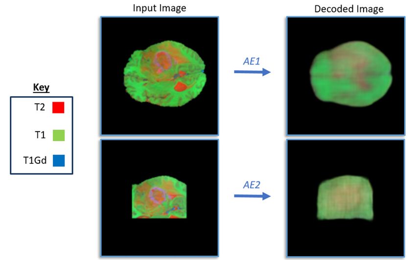
Abstract
Magnetic Resonance Imaging (MRI) is commonly used in the diagnosis of brain tumors. Traditionally, physicians are
trained to use their eyes when interpreting the scans; as the old saying goes, “a radiologist looking for a ruler is
a radiologist in trouble.” The recent emergence of the field of radiomics – which quantifies tumor features in MRI
scans to create mineable high-dimensional data – is changing the game and creating new clinical decision support
tools for identifying cases with tumor similarities. This paper leverages deep learning to match MRI tumor images to
scans with similar features with the goal of providing clinicians a tool to increase accuracy and speed to diagnosis.
The methodology presented herein involves combining multiple artificial neural networks in order to identify tumor
regions and then match the tumor in question to those with the highest degree of similarities.

Business Justification
Magnetic resonance imaging (MRI) is a common medical imaging tool used to diagnose a variety of conditions, such
                1
as brain cancer . The rich information composed in MRI imaging data can reveal valuable insights into diagnosis and
recommended treatment options. When first introduced into clinical practice, MRI images were manually interpreted
by radiologist in a time intensive visual review process. Recently, the field of radiomics has emerged which transforms
MRI images into mineable high-dimensional data, enabling physicians to harness quantitative image analysis that aid
                                2,3
the clinical decision process .

While radiomics can provide quantitative patient information, the timely step of isolating specific regions
                                                                                         4
(segmentation) is required to improve the features extracted by radiometric methods . For example, in interpreting
scans for cancer diagnosis, the physician is often interested in tumor characteristics and not the surrounding healthy
tissue. Therefore, physicians must first select a region of interest (ROI) so that the radiomic quantitative metrics
have clinical relevance to the tumor and not the entire imaging area. With the current lack of trained radiologists,
especially in rural areas, the automation of the ROI segmentation process could prove beneficial to tumor
                                           5
identification and the radiomics pipeline .

Convolutional neural networks (CNNs) have been shown as a promising automated solution to the ROI selection
                          4–6
process and radiometrics        . CNNs extract image features through multiple layers of convolution with trainable
        7
weights . The CNN is trained to identify ROIs by learning from human-labeled segmented images, placing ROI
segmentation CNNs in a type of deep learning called supervised learning (i.e., supplying the CNN with labels
is required). Once trained, the CNN can rapidly identify ROIs on images it was not trained on. Common CNN
architectures to perform ROI selection are YOLO (You only look once) and U-nets, among others. On an average,
it takes a physician about one hour to segment a brain tumor; however CNNs have been shown to segment brain
                                                                  8
tumors in under one minute with similar accuracy to physicians . Therefore, it can be seen how CNNs are crucial to
the ROI selection process for radiomics and can help to address the radiologist shortage problem.

                                                                                                          MRI Radiomics   3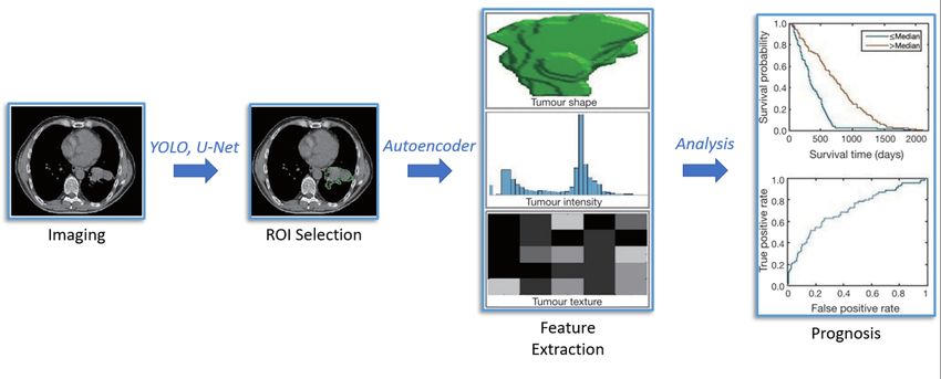
In addition to segmentation, CNNs can also allow clinically relevant features to be extracted from the ROIs for
radiomics. A popular CNN architecture for extracting relevant features is a CNN autoencoder. Autoencoders
compress images down into an encoding, which contain the relevant clinical features. For example, when supplied
with an ROI of a tumor the autoencoder compresses the image down to an encoding which contains clinically
relevant features such as texture that can be later used for prognosis analysis9. Unlike ROI segmentation CNNs,
autoencoders are a type of unsupervised learning and only need to be supplied with an image for training, reducing
the cost and time associated with relevant feature extraction in the radiomics pipeline.

The extracted features from CNN autoencoders can often be abstract and difficult for a human to interpret. To
obtain useful information to aid in clinical decisions, the extracted features must be analyzed and compared with
other patient data in a large database. For example, the embedding of a patient of interest can be compared against
the embeddings of other patients to find similar cases. By comparing treatments and outcomes of similar cases the
feature analysis can aid the physician in a clinical decision. Feature analysis takes just seconds, whereas a physician
can spend up to an hour comparing similar cases (and always with the possibility of missing relevant cases based
on nuanced feature similarities). Feature analysis is a large area of research and can be performed using a variety of
                                                                                                  9
machine learning techniques such as deep learning, support vector machines or decision trees .

  Figure 1
  Implementation of CNNs into radiomics pipeline. CNNs
  such as YOLO or U-net are used to identify the tumor
  ROI. The relevant clinical features are then extracted to
  an embedding using a CNN autoencoder. Finally, the
  features are analyzed to aid physicians in prognosis.

In this paper an MRI brain tumor radiomics pipeline solution is described that can provide physicians with a similar
patient case in under a minute, potentially saving physicians hours of work and creating a meaningful mechanism for
clinical decision support. A YOLO CNN is employed to identify brain tumors, and two CNN autoencoders to identify
patients with similar tumors. For training of the CNNs and generating a lookup database the 2020 BraTS (Brain Tumor
Image Segmentation Benchmark) database was utilized. Provided by the Perelman School of Medicine at University
of Pennsylvania, the BraTS database is an image database that contains brain tumor segmentations and four MRI
                        10–12
modalities per patient          .

                                                                                                         MRI Radiomics    4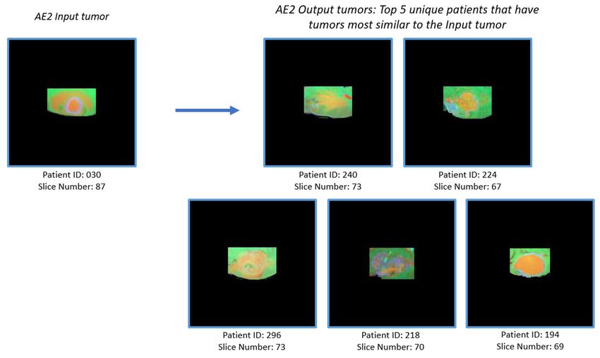
Experimental Setup and Methodology
Dataset

The BraTS 2020 dataset consists of 494 patients, each with a full MRI brain scan across four different MRI
modalities: T1, T1Gd, T2 and T2-FLAIR (Fluid Attenuated Inversion Recovery). In brief, MRI obtains image contrast
by applying a variety of magnetic pulses to tissue and sensing the resulting changes to proton particles’ spin. T1,
T2 and T2-FLAIR each apply different magnetic pulses to look at tissue proton spin changes, while T1Gd applies
a T1 pulse after intravenously infusing the patient with the contrast agent Gadolinium10. Since each modality
applies a different magnetic pulse or uses a contrast agent, they each reveal different clinically relevant structural
and molecular contrast information about the tissue. The BraTS dataset was created to allow data scientists
to compete in developing the best radiomic algorithms. So, for 369 patients in the dataset there are three-
dimensional (3D) segmentations of the tumor (if one is present and manual generated by human experts), as well
as additional metadata such as overall patient survival and tumor characteristics. For the remaining 125 patients
this additional information is left out and only known by the providers of the BraTS dataset. For the purposes of this
work, only the MRI brain scans and tumor segmentations were used for training of CNNs and the 125 patients with
missing segmentation information were used for testing. Each MRI modality and tumor segmentation contains a
155x240x240 pixel data cube in NIFTY format. All modalities and segmentations are co-registered for each patient.
An example of different modalities and the segmented tumor are provided in the Figure 2.

  Figure 2
  Example MRI slice of patient with a brain tumor from the BraTS 2020
  dataset. Showing all four modalities as well as the human expert
  produced tumor segmentation.

While the dataset contained 3D data for each modality, the CNNs only use one slice at a time along the second and
third dimensions (Transverse Plane) of the data cube. So, for each patient and modality there are 155 slices or images
of size 240x240 pixels.

                                                                                                         MRI Radiomics   5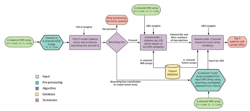
Radiomics Pipeline Architecture

The objective of the radiomics pipeline (Figure 3) presented in this paper is to take a patient MRI slice, identify if a
tumor is present, and if one is present find a patient slice with a similar tumor. The user supplies the pipeline with
a patient MRI slice, where YOLO will then detect a tumor ROI if one is present. If no tumor is present, the pipeline
finishes. If a tumor is present, autoencoder 1 (AE1) extracts the relevant image features across the whole slice and
compares it with other patient slice features in the database. Notice that in the autoencoder approach, features
are automatically generated as a result of the autoencoder’s inherent dimensional reduction, without necessitating
explicit definition or selection. The top 200 slice results are then identified. Next, the tumor is segmented from the
supplied slice using YOLO and the features are extracted with autoencoder 2 (AE2). The tumor features are then
compared with the tumor features from the top 200 slice results of AE1, and the top five results from unique patients
are output.

It is common practice in medicine to use different MRI modalities in a complementary way to extract maximum and
                      6
highly useful features . Therefore, YOLO and the autoencoders were supplied with multi-modal images to maximize
relevant feature extraction and radiomic performance. YOLO is supplied with T1, T2, T1Gd slices, while AE1 and AE2
are supplied with all modalities. YOLO only used three modalities so prebuilt YOLO models (which typically take red,
green, blue three channel images) can be used and transfer learning can be taken advantage of to speed up training.
For the autoencoders, custom networks were built to accept all four MRI modalities.

  Figure 3
  Radiomics Pipeline Architecture

                                                                                                           MRI Radiomics   6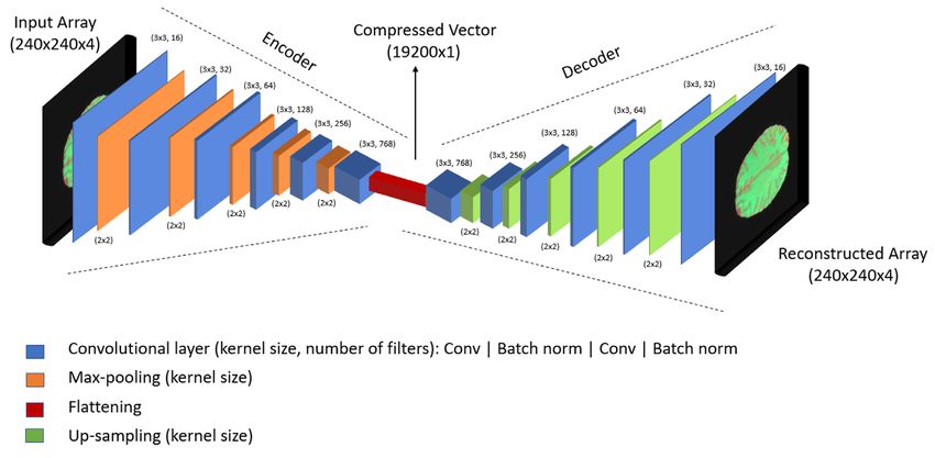
YOLOV3 Model
YOLO, which expands to “You Only Look Once,” is an object detection and identification algorithm that is based
on CNNs. One of YOLO’s key benefits is that it can detect multiple objects of different categories by only scanning
the image one time, hence the name “you only look once.” This allows YOLO to infer object detection quickly, ~50
milliseconds on a graphical processing unit (GPU). In this project, YOLOv3 model was used which was supplied
with pretrained weights to expedite training time and available at this GitHub location: github.com/AntonMu/
13
TrainYourOwnYOLO/tree/master . All the YOLO training was performed on Amazon Web Services (AWS) p3.8xlarge
instance using a dockerized TensorFlow image. The docker image used was tensorflow/tensorflow:nightly-custom-
op-gpu-ubuntu16 and was pulled from the docker hub (hub.docker.com).
In this project, YOLO is used to detect and locate brain tumors from the MRIs. To train YOLO it needs to be supplied
with MRI images and their respective tumor bounding box locations. The BraTS dataset supplied a binary 3D tumor
mask. Each mask consists of complex 3D shapes that are often disconnected. These masks need to be converted
into a bounding box to train YOLO for each slice. To do this the following steps were taken:
1. A slice of the binary tumor mask is read and dilated with 5x5 kernel to connect sparse tumor masks.
2. Connected component analysis is performed to find all tumor locations in the slice. Connected components
with less than 300 pixels are filtered out to allow for sufficient signal in YOLO training.
3. For each connected component or tumor the contour extremes are found and used to calculate the bounding
box coordinates.
As discussed earlier in the pipeline architecture, the training images for YOLO were created using three modalities,
T2, T1 and T1Gd. YOLOv3 takes Red-Green-Blue channel images as input, thus 240x240x3 arrays for each slice were
created using the three modalities for the third dimension. Labels for training YOLO were supplied in CSV (comma
separated values) format with the following information: multi-modal slice image name, bounding box coordinates,
and the object name (in this application only 1 category was used: Brain Tumor). The bounding box coordinates were
created for the CSV using the tumor mask to bounding box steps described above.
YOLO was trained on a total of 24,422 multi-modal MRI images. Out of training data (228,780 images), approximately
10.6% images had tumor(s) in them. The validation loss after training was 7.84. Once trained when supplied with
the three-channel multi-modal MRI image, YOLO was able to identify where a tumor was located along with the
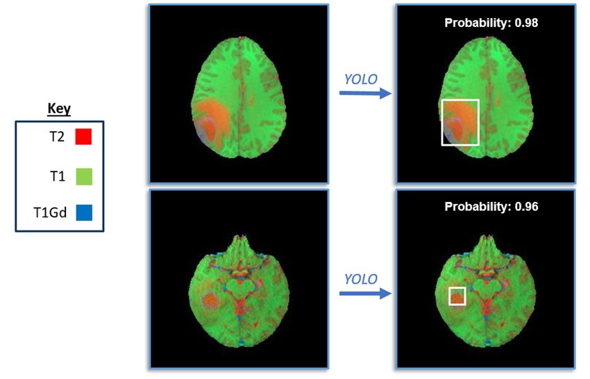
probability of it being a tumor (as shown in Figure 4).
MRI Radiomics 7Figure 4
YOLO identification of tumors from multi-modal MRI images. Key
describes the color channel used to represent the intensity of the
image from each MRI modality.
Autoencoders
The purpose of autoencoders in the radiomics pipeline was to extract relevant image features needed to find similar
images in the BraTS database. The autoencoders compressed multi-modal MRI images into an encoded vector
which contained the relevant image features. Both autoencoders, AE1 and AE2, were built on the same architecture
(Figure 5). The input was a 240x240x4 image where the third dimension was the different MRI modalities. The
encoded vector, which contained the relevant image features, was 19200x1. Therefore, the autoencoder compressed
the input multi-modal MRI images into encodings with a compression ratio of 12.
The Python package Keras was used to construct and train the autoencoders. Unlike YOLO, the autoencoders
used the input image as a label and compared it with the image output by the autoencoder to train weights. The
autoencoder architecture consisted of 12 layers: six layers for the encoder and six layers for the decoder parts of the
network (as shown in Figure 5 below). Each layer had two convolutional layers, followed by batch normalization and
14
max pooling for encoding or up-sampling for decoding. Batch normalization was performed to expedite training . To
obtain the encoded vector, flattening was performed in the final layer of the encoder. This resulted in a large network
with a total of 21 million trainable parameters.
MRI Radiomics 8Figure 5
Autoencoder Architecture
These Keras callbacks were used for model tuning:
1. ModelCheckpoint: For saving the weights for each epoch of training and monitoring the validation loss. 14
2. EarlyStopping: To avoid overfitting, the validation loss was monitored. If the validation loss did not improve over
10 epochs the training was terminated.
Both the autoencoders were compiled with Adadelta optimizer and binary cross-entropy loss. A mini-batch size of
100 images was used.
The autoencoder was trained on an AWS p3.8xlarge instance using two Tesla V100 GPUs, one for each autoencoder.
It took about 50 hours to complete the autoencoder training. However, it should be noted that the validation loss did
not stagnate and even after 50 hours of training further improvement could potentially be realized.
I. AE1
AE1 was used to identify similar MRI slices. After training AE1, the validation loss reached a value of 0.12. The generated
image from the decoder can be compared with the input image to visualize how the autoencoder was performing (as
shown in Figure 6). The autoencoder successfully extracted some relevant image features. While the decoded image is
blurry there appears to be similarities between the input and output image modality intensity regions and the outline of
the brain is consistent.
To find similar slices of a test multi-modal MRI image, its compressed vector from AE1 is compared with other slices’
compressed vectors in the BraTS database. Cosine similarity ranking was used to measure the similarity between the
input test image and the compressed vectors in the database. Cosine similarity takes a maximum value of one, and the
higher the value, the more similar the two compressed vectors are. To expedite lookup of test images, all the BraTS
training images were pre-compressed into their encoded vectors. Cosine similarity was then calculated between the
test image and all the training images using batches of 100 compressed vectors and TensorFlow’s cosine similarity
function utilizing a GPU. We found that the top similar slice results would often be from the same patient. Since the end
goal of the pipeline was to find patients with a similar tumor, the top ranked slices from the top 200 MRI slices were
filtered to be fed into AE2. Among these 200 slices, the top five individual patients are obtained that have the highest
MRI Radiomics 9similarity in full-MRIs.
II. AE2
AE2 was used to find similar tumors within the top ranked slices from the top 200 MRI slices obtained from
section above. The generated image from the decoder can be compared with the input image to visualize how the
autoencoder was performing (as shown in Figure 6). After training AE2, the validation loss reached a value of 0.03.
Like AE1, the performance of AE2 can be visualized by comparing the input and output image. AE2 successfully
extracted some relevant features which allowed similar tumors to be identified.
To prepare the data fed into AE2, the tumors were cropped using the bounding boxes from YOLO and centered in
a 240x240x4 array of zeros. This ensured that the tumors fed into AE2 were all the same size and the autoencoder
input layer could remain constant.
To find similar tumors, the input test image was cropped according to YOLO output and fed into AE2 to obtain the
encoding vectors. The test image was then compared and ranked against the top 200 encoded vectors using cosine
similarity. The top five results from individual patients were then output that had similar tumors as that of the input.
Figure 6
Multi-modal MRI image and generated output image from AE1 and AE2. Only 3 of the 4 modalities are shown to allow it
to be visualized as a red, green, blue image. It can be seen the autoencoders are able to maintain some relevant image
features even after 12x compression, suggesting important imaging features have been extracted which can be used to
find images with similar features.
.
MRI Radiomics 10Results
Autoencoders’ Results
After training, the validation losses of both autoencoders were as follows:
1. AE1: 0.12
2. AE2: 0.03
These relatively low values for the binary cross entropy from the autoencoders indicate that the encoders are able to
successfully compress the information contained in the MRI’s while maintaining a faithful description of the original
image.
Tumor Detection Results
After training, the validation loss for the YOLO model reached 7.84. The trained YOLO model was used to detect
tumors in 9165 new MRIs. The model found tumors in 6014 of these MRIs. The mean of the confidence scores by
which the YOLO model detected tumor(s) is 85.7%. Out of all the MRIs in which the algorithm detected tumors, more
than 60% of them had a confidence score of at least 95%.
Image Lookup Results
The image lookup code was built to identify MRIs that showed similarities, both, in the complete MRI slice and in the
tumor image (if any). This code was run on AWS using p2.xlarge instance and on average, it took 47.6 seconds to
execute completely. These results demonstrate the impact our model can have in segmenting brain tumors and in
providing MRI and tumor slices that are most similar to the input MRI.
Figure 7 is an example of the inputs and outputs of the image lookup code:
Figure 7(a)
MRI Radiomics 11Figure 7(b)
Figure 7
(a) Example Inputs and outputs to AE1. The output consists of MRI slices of 5 unique patients having MRIs most similar to
the input slice. (b) Example Inputs and outputs to AE2. The output consists of tumor slices (cropped from the MRI slices) of
5 unique patients having tumors most similar to the input tumor.
In these examples, we observe qualitative similarity of the brain MRI slices in the images returned in Figure 7(a) as well
as the tumors shape and size for the images in Figure 7(b). These results indicate to us that the two autoencoders
are producing good representations of the brain MRI’s which allows for successful reverse image lookup.
MRI Radiomics 12Conclusion
We developed an MRI brain tumor radiomics pipeline solution that could increase accuracy and speed to diagnosis
by providing physicians with a similar patient MRI images in under a minute. This pipeline employs a YOLO CNN to
identify brain tumors, and two CNN autoencoders to first identify similar patient MRI slices, and then within those
similar patient slices, to identify patients with similar tumors. The YOLO CNN produced a validation loss of 7.84, and
the two autoencoders produced validation losses of 0.12 and 0.03 respectively.
There are several important considerations that need to be made when deploying a robust implementation of this
pipeline. For example, our pipeline employs the black box approach—images are inputted, and similar images are
received as output, but the actual decisions made by the algorithm are opaque to the user. The pipeline would
benefit from an increase in interpretability, perhaps, by including the feature importance in the model decision
making process. Also, as noted above, the autoencoder loss was not stagnating. Further increase in performance can
be obtained by training the autoencoders for a longer period. Finally, a U-Net CNN can be more accurate than YOLO
because U-Net produces a well-defined border around the tumor, while YOLO produces a bounding box.
MRI Radiomics 13References
1. Shukla, G. et al. Advanced magnetic resonance imaging in glioblastoma: A review. Chinese Clin. Oncol. 6, 1–12
(2017)..
2. Lambin, P. et al. Radiomics: The bridge between medical imaging and personalized medicine. Nat. Rev. Clin. Oncol.
14, 749–762 (2017).
3. Kumar, V. et al. Radiomics: The process and the challenges. Magn. Reson. Imaging 30, 1234–1248 (2012).
4. Feng, X., Tustison, N. J., Patel, S. H. & Meyer, C. H. Brain Tumor Segmentation Using an Ensemble of 3D U-Nets and
Overall Survival Prediction Using Radiomic Features. Front. Comput. Neurosci. 14, 1–12 (2020).
5. Rahman, T. et al. Transfer Learning with Deep Convolutional Neural Network (CNN) for Pneumonia Detection Using
Chest X-ray. Appl. Sci. 10, 3233 (2020).
6. Iqbal, S., Ghani, M. U., Saba, T. & Rehman, A. Brain tumor segmentation in multi-spectral MRI using convolutional
neural networks (CNN). Microsc. Res. Tech. 81, 419–427 (2018).
7. LeCun, Y. et al. Backpropagation Applied to Handwritten Zip Code Recognition. Neural Comput. 1, 541–551 (1989).
8. naceur, M. Ben, Saouli, R., Akil, M. & Kachouri, R. Fully Automatic Brain Tumor Segmentation using End-To-End
Incremental Deep Neural Networks in MRI images. Comput. Methods Programs Biomed. 166, 39–49 (2018).
9. Vial, A. et al. The role of deep learning and radiomic feature extraction in cancer-specific predictive modelling: A
review. Transl. Cancer Res. 7, 803–816 (2018).
10. Menze, B. H. et al. The Multimodal Brain Tumor Image Segmentation Benchmark (BRATS). IEEE Trans. Med.
Imaging 34, 1993–2024 (2015).
11. Bakas, S. et al. Identifying the Best Machine Learning Algorithms for Brain Tumor Segmentation, Progression
Assessment, and Overall Survival Prediction in the BRATS Challenge. Physiol. Behav. 176, 139–148 (2018).
12. Bakas, S. et al. Advancing The Cancer Genome Atlas glioma MRI collections with expert segmentation labels and
radiomic features. Sci. Data 4, 1–13 (2017).
13. Redmon, J. & Farhadi, A. YOLOv3: An incremental improvement. arXiv (2018).
MRI Radiomics 14Learn more about WWT’s Artificial Intelligence Research & Development at:
https://www.wwt.com/artificial-intelligence-research-and-development
About WWT Artificial Intelligence Research & Development
The Artificial Intelligence Research & Development program at WWT is an applied research initiative focused on
investigating the one to three-year horizon of the artificial intelligence space. The AI R&D program conducts internal
projects grounded in WWT’s deep understanding of industry use cases and produces reusable components and
white papers to share with customers and the AI community.
Through strategic partnerships, cutting-edge data science and ML Ops skills, and ability to test and learn in the
Advanced Technology Center and public cloud, the AI R&D team advances WWT’s knowledge of the AI and ML
space, thus allowing WWT to be on the bleeding edge and remain strategic advisors to businesses in their AI needs.
About WWT
Founded in 1990, WWT has grown to become a global technology solution provider with $13.4 billion in annual
revenue. With thousands of IT engineers, hundreds of application developers and unmatched labs for testing and
deploying technology at scale, WWT helps customers bridge the gap between IT and the business. By bringing
leading technology companies together in a physical yet virtualized environment through its Advanced Technology
Center, WWT integrates individually impressive technologies to produce game-changing solutions.
Based in St. Louis, WWT employs 7,000 employees and operates more than 4 million square feet of warehousing,
distribution and integration space in more than 20 facilities throughout the world.
MRI Radiomics 15You can also read