Multi-Session Visual SLAM for Illumination Invariant Localization in Indoor Environments
←
→
Page content transcription
If your browser does not render page correctly, please read the page content below
Multi-Session Visual SLAM for Illumination Invariant Localization in
                                                                 Indoor Environments
                                                                                         Mathieu Labbé and François Michaud

                                           Abstract— For robots navigating using only a camera, illumi-               •  Which visual feature is the most robust to illumination
                                        nation changes in indoor environments can cause localization                     variations?
                                        failures during autonomous navigation. In this paper, we                       • How many sessions are required for robust localization
                                        present a multi-session visual SLAM approach to create a map
                                        made of multiple variations of the same locations in different                   through day and night based on the visual feature
                                                                                                                         chosen?
arXiv:2103.03827v1 [cs.RO] 5 Mar 2021

                                        illumination conditions. The multi-session map can then be used
                                        at any hour of the day for improved localization capability.                   • To avoid having a human teleoperate a robot at different
                                        The approach presented is independent of the visual features                     times of the day to create the multi-session map, would
                                        used, and this is demonstrated by comparing localization                         it be possible to acquire the consecutive maps simply
                                        performance between multi-session maps created using the
                                        RTAB-Map library with SURF, SIFT, BRIEF, FREAK, BRISK,                           by having localization be done using the map acquired
                                        KAZE, DAISY and SuperPoint visual features. The approach                         from the previous session?
                                        is tested on six mapping and six localization sessions recorded                The paper is organized as follows. Section II presents
                                        at 30 minutes intervals during sunset using a Google Tango                  similar works to our multi-session map approach, which is
                                        phone in a real apartment.
                                                                                                                    described in Section III. Section IV presents comparative
                                                              I. INTRODUCTION                                       results between the visual feature used and the number of
                                                                                                                    sessions required to expect the best localization performance.
                                           Visual SLAM (Simultaneous Localization and Mapping)                      Section V concludes with limitations and possible improve-
                                        frameworks using hand-crafted visual features work rela-                    ments of the approach.
                                        tively well in static environments, as long as there are
                                        enough discriminating visual features with moderated light-                                   II. RELATED WORK
                                        ing variations. To be illumination invariant, a trivial solution               The most similar approach to the one presented in this
                                        could be to switch from vision to LiDAR (Light Detection                    paper exploits what is called an Experience Map [2]. An
                                        and Ranging) sensors, but they are often too expensive for                  experience is referred to an observation of a location at a
                                        some applications in comparison to cameras. Illumination-                   particular time. A location can have multiple experiences
                                        invariant localization using a conventional camera is not                   describing it. New experiences of the same location are
                                        trivial, as visual features taken during the day under nat-                 added to the experience map if localization fails during
                                        ural light conditions may look quite different than those                   each traversal of the same environment. Localization of the
                                        extracted during the night under artificial light conditions.               current frame is done against all experiences in parallel, thus
                                        In our previous work on visual loop closure detection [1],                  requiring multi-core CPUs to do it in real-time as more and
                                        we observed that when traversing multiple times the same                    more experiences are added to a location. To avoid using
                                        area where atmospheric conditions are changing periodically                 multiple experiences of the same locations, SeqSLAM [3],
                                        (like day-night cycles), loop closures are more likely to                   [4] matches sequences of visual frames instead of trying to
                                        be detected with locations of past mapping sessions that                    localize robustly each individual frame against the map. The
                                        have similar illumination levels or atmospheric conditions.                 approach assumes that the robot takes relatively the same
                                        Based on that observation, in this paper, we present an                     route (with the same viewpoints) at the same velocity, thus
                                        multi-session approach to derive illumination invariant maps                seeing the same sequence of images across time. This is a
                                        using a full visual SLAM approach (not only loop closure                    fair assumption for cars (or trains), as they are constrained
                                        detection). Mapping multiple times the same area to improve                 to follow a lane at regular velocity. However, for indoor
                                        localization in dynamic environments has been tested more                   robots having to deal with obstacles, their path can change
                                        often outdoors with cars on road constrained trajectories [2],              over time, thus not always replicating the same sequences
                                        rather than indoors in unconstrained trajectories where the                 of visual frames. In Cooc-Map [5], local features taken at
                                        full six Degrees of Freedom (DoF) transformations must also                 different times of the day are quantized in both the feature
                                        be recovered. The main questions this paper addresses are:                  and image spaces, and discriminating statistics can be gener-
                                                                                                                    ated on the co-occurrences of features. This produces a more
                                           *This work is partly supported by the Natural Sciences and Engineering
                                        Research Council of Canada.                                                 compact map instead of having multiple images representing
                                           Mathieu Labbé and François Michaud are with Interdisciplinary          the same location, while still having local features to recover
                                        Institute of Technological Innovation (3IT), Department of                  full motion transformation. A similar approach is done in [6]
                                        Electrical Engineering and Computer Engineering, Université de
                                        Sherbrooke, Sherbrooke, Québec, Canada [Mathieu.M.Labbe                    where a fine vocabulary method is used to cluster descriptors
                                        | Francois.Michaud]@USherbrooke.ca                                          by tracking the corresponding 3D landmark in 2D images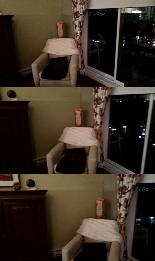
Localization
across multiple sequences under different illumination con-                         01:00
                                                                                                                       Session B
ditions. For feature matching with this learned vocabulary,
instead of using a standard descriptor distance approach (e.g.,                     00:00
                                                                                              Map3
Euclidean distance), a probability distance is evaluated to                                                           Multi-Session
                                                                                    18:00
improve feature matching. Other approaches rely on pre-                                            Map2                   Map

processing the input images to make them illumination-
                                                                                    12:00
                                                                                            Map1
invariant before feature extraction, by removing shadows [7],
[8] or by trying to predict them [9]. This improves feature                         16:00
                                                                                                                        Localization
                                                                                                                         Session A
matching robustness in strong and changing shadows.
   At the local visual feature level, common hand-crafted
                                                                    Fig. 1. Structure of the multi-session map. Three sessions taken at different
features like SIFT [10] and SURF [11] in outdoor ex-                time have been merged together by finding loop closures between them
periences can be compared across multiple seasons and               (yellow links). Each map has its own coordinate frame. Localization Session
illumination conditions [12], [13]. To overcome limitations         A (16:00) is localized in relation to both day sessions, and Localization
                                                                    Session B (01:00) is only for the night session (00:00).
caused by illumination variance of hand-crafted features,
machine learning approaches have been also used to extract
descriptors that are more illumination-invariant. In [14], a
neural network has been trained by tracking interest points in      implicitly transform each session into the coordinate frame
time-lapse videos, so that it outputs similar descriptors for the   of the oldest map as long as there is at least one loop closure
same tracked points independently of illumination. However,         found between the sessions.
only descriptors are learned, and the approach still relies            RTAB-Map uses two methods to find loop closures: a
on hand-crafted feature detectors. More recently, SuperPoint        global one called loop closure detection, and a local one
[15] introduced an end-to-end local feature detection and           called proximity detection. For multi-session maps, loop
descriptor extraction approach based on a neural network.           closure detection works exactly the same than with single
The illumination-invariance comes from carefully making a           session maps. The bag-of-words (BOW) approach [1] is used
training dataset with images showing the same visual features       with a Bayesian filter to evaluate loop closure hypotheses
under large illumination variations.                                over all previous images from all sessions. When a loop
                                                                    closure hypothesis reaches a pre-defined threshold, a loop
 III. MULTI-SESSION SLAM FOR ILLUMINATION                           closure is detected. Visual features can be any of the ones im-
          INVARIANT LOCALIZATION                                    plemented in OpenCV [19], which are SURF (SU) [11], SIFT
   Compared to an experience map, our approach also ap-             (SI) [10], BRIEF (BF) [20], BRISK (BK) [21], KAZE (KA)
pends new locations to the map during each traversal, but it        [22], FREAK (FR) [23] and DAISY (DY) [24]. Specifically
estimates only the motion transformation with a maximum             for this paper, the neural network based feature SuperPoint
of best candidates based on their likelihood. Our approach          (SP) [15] has also been integrated for comparison. The BOW
is also independent of the visual features used, which can be       vocabulary is incremental based on FLANN’s KD-Trees [25].
hand-crafted or neural network based, thus making it easier         Quantization of features to visual words is done using the
to compare them in full SLAM conditions using RTAB-                 Nearest Neighbor Distance Ratio (NNDR) approach [10].
Map library for instance. RTAB-Map [16] is a Graph-SLAM                In our previous works [26], proximity detection was
[17] approach that can be used with camera(s) and/or with           introduced primarily in RTAB-Map for LiDAR localization.
a LiDAR. This paper focuses on the first case where only            A slight modification is made for this work to use it with
a camera is available for localization. The structure of the        a camera. Previously, closest nodes in a fixed radius around
map is a pose-graph with nodes representing each image              the current position of the robot were sorted by distance,
acquired at a fixed rate and links representing the 6DoF            then proximity detection was done against the top three
transformations between them. Figure 1 presents an example          closest nodes. However, in a visual multi-session map, the
of a multi-session map created from three sessions taken at         closest nodes may not have images with the most similar
three different hours. Two additional localization sessions         illumination conditions than the current one. By using the
are also shown, one during the day (16:00) and one at               likelihood computed during loop closure detection, nodes
night (01:00). The dotted links represent to which nodes            inside the proximity radius are sorted from the most to less
in the graph the corresponding localization frame has been          visually similar (in terms of BOW’s inverted index score).
localized on. The goal is to have new frames localize on            Visual proximity detection is then done using the three most
nodes taken at a similar time, and if the localization time         similar images around the current position. If proximity
falls between two mapping times, localizations could jump           detection fails because the robot’s odometry drifted too much
between two sessions or more inside the multi-session map.          since the last localization, loop closure detection is still done
Inside the multi-session map, each individual map must be           in parallel to localize the robot when it is lost.
transformed in the same global coordinate frame so that                For both loop closure and proximity detections, 6DoF
when the robot localizes on a node of a different session,          transformations are computed in two steps: 1) a global
it does not jump between different coordinate frames. To do         feature matching is done using NNDR between frames to
so, the GTSAM [18] graph optimization approach is used to           compute a first transformation using the Perspective-n-Point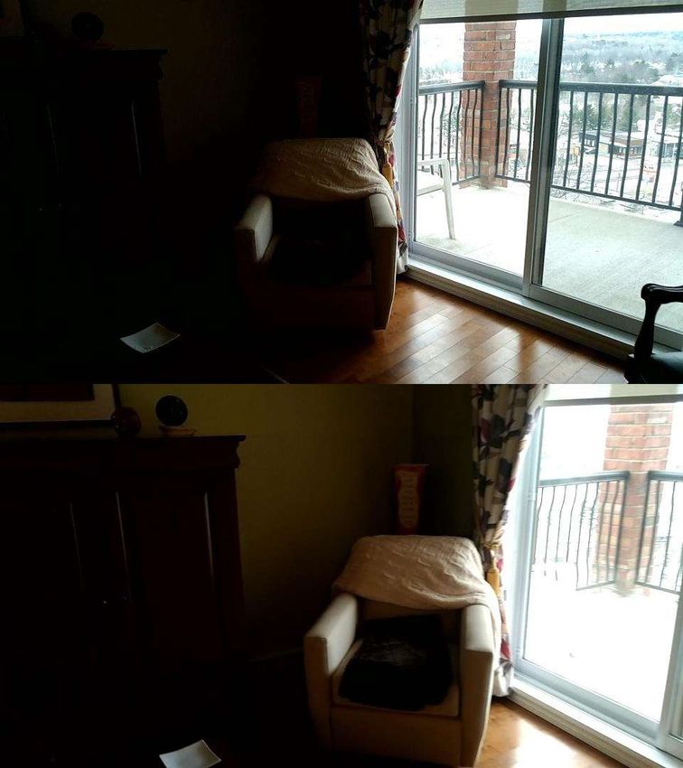
(PnP) approach [19]; then 2) using that previous transforma- of the six localization sessions (A to F) using the visual
tion as a motion estimate, 3D features from the first frame are features listed in Section III. As expected by looking at the
projected into the second frame for local feature matching diagonals, localization performance is best (less gaps) when
using a fixed size window. This second step generates better localization is done using a map taken at the same time of
matches to compute a more accurate transformation using the day (i.e., with very similar illumination condition). In
PnP. The resulting transform is further refined using the local contrast, localization performance is worst when localizing at
bundle adjustment approach [27]. night using a map taken the day, and vice-versa. SuperPoint
is the most robust to large illumination variations, while
IV. RESULTS binary descriptors like FREAK, BRIEF and BRISK are the
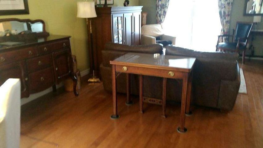
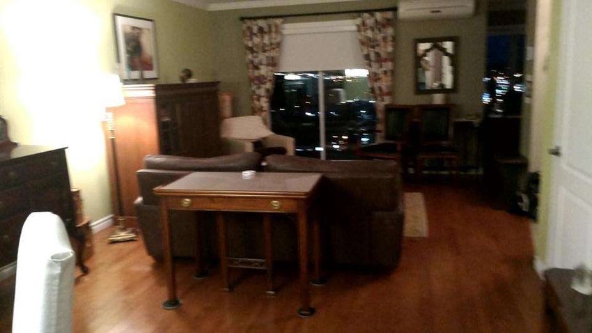
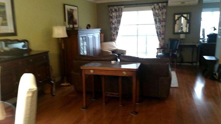
Figure 2 illustrates how the dataset has been acquired most sensitive.
in a home in Sherbrooke, Quebec in March. An ASUS
Zenfone AR phone (with Google Tango technology) running B. Multi-Session Localization
a RTAB-Map Tango App has been used to record data for The second experiment evaluates localization performance
each session following the same yellow trajectory, similarly using multi-session maps created using maps generated at
to what a robot would do patrolling the environment. The different times from the six mapping sessions. Different
poses are estimated using Google Tango’s visual inertial combinations are tested: 1+6 combines the two mapping
odometry approach, with RGB and registered depth images sessions with the highest illumination variations (time 16:46
recorded at 1 Hz. The trajectory started and finished in front with time 19:35); 1+3+5 and 2+4+6 are multi-session maps
of a highly visual descriptive location (i.e., first and last generated by assuming that mapping would occur every 1
positions shown as green and red arrows, respectively) to hour instead of every 30 minutes, and 1+2+3+4+5+6 is the
make sure that each consecutive mapping session is able combination of all maps. Figure 4 illustrates, from top to
to localize on start from the previous session. This makes bottom and for each multi-session map the resulting local-
sure that all maps are transformed in the same coordinate ized frames over time. Except for SuperPoint which shows
frame of the first map after graph optimization. For each run similar performance for all multi-session maps, sessions with
between 16:45 (daylight) and 19:45 (nighttime), two sessions different illumination conditions merged together increase
were recorded back-to-back to get a mapping session and a localization performance. For the case 1+2+3+4+5+6 (fourth
localization session taken roughly at the same time. The time line), localization sessions at 16:51 and at 19:42 are local-
delay between each run is around 30 minutes during sunset. izing mostly with sessions taken at the same time (1 and
Overall, the resulting dataset has six mapping sessions (1- 6), while for other sessions, localizations are mixed between
16:46, 2-17:27, 3-17:54, 4-18:27, 5-18:56, 6-19:35) and six more than one maps. This confirms that these two are the
localization sessions (A-16:51, B-17:31, C-17:58, D-18:30, most different ones in the set of multi-map combinations.
E-18:59, F-19:42). Table I presents cumulative localization performance over
The top blue boxes of Fig. 2 show images of the same single session and multi-session maps for each visual fea-
location taken during each mapping session. To evaluate ture. As expected, multi-session maps improves localization
the influence of natural light coming from the windows performance. The map 1|2|3|4|5|6 corresponds to the case
during the day, all lights in the apartment were on during all of only using the session map taken at the closest time
sessions except for one in the living room that we turned on of the localization session. While this seems to result in
when the room was getting darker (see top images at 17:54 similar performance compared to the multi-session cases,
and 18:27). Beside natural illumination changing over the this could be difficult to implement robustly over multiple
sessions, the RGB camera had auto-exposure and auto-white seasons (where general illumination variations would not
balance enabled (which could not be disabled by Google always happen at the same time) and during weather changes
Tango API on that phone), causing additional illumination (cloudy, sunny or rainy days would result in changes in
changes based on where the camera was pointing, as shown illumination conditions for the same time of day). Another
in the purple box of Fig. 2. The left sequence illustrates challenge is how to make sure that maps are correctly
what happens when greater lighting comes from outside, aligned together in same coordinate frame during the whole
with auto-exposure making the inside very dark when the trajectory. In contrast, with the multi-session approach, the
camera passed by the window. In comparison, doing so selection of which mapping session to use is done implicitly
at night (shown in the right sequence) did not result in by selecting the best candidates of loop closure detection
any changes. Therefore, for this dataset, most illumination across all sessions. There is therefore no need to have a priori
changes are coming either from natural lighting or auto- knowledge of the illumination conditions during mapping
exposure variations. before doing localization.
However, the multi-session approach requires more mem-
A. Single Session Localization ory usage, as the map is at most six times larger in our
The first experiment done with this dataset examines experiment than a single session of the same environment.
localization performance of different visual features for a Table II presents the memory usage (RAM) required for
single mapping session. Figure 3 shows for each single localization using the different maps configurations, along
session map (1 to 6) the resulting localized frames over time with the constant RAM overhead (e.g., loading libraries
16:46 17:27 17:54 18:27 18:56 19:35
17:27 19:35
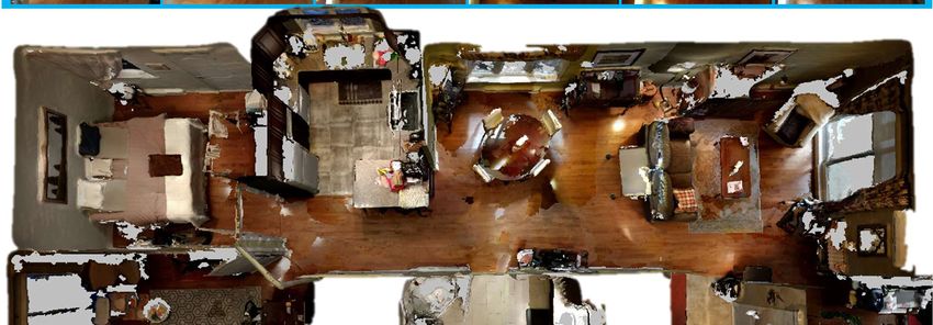
Fig. 2. Top view of the testing environment with the followed trajectory in yellow. Start and end positions correspond to green and red triangles
respectively, which are both oriented toward same picture on the wall shown in the green frame. Circles represent waypoints where the camera rotated
in place. Windows are located in the dotted orange rectangles. The top blue boxes are pictures taken from a similar point of view (located by the blue
triangle) during the six mapping sessions. The purple box shows three consecutive frames from two different sessions taken at the same position (purple
triangle), illustrating the effect of auto-exposure.
16:51 17:31 17:58 18:30 18:59 19:42 16:51 17:31 17:58 18:30 18:59 19:42
16:46 16:46
SURF 17:27 SURF 17:27
17:54 17:54
18:27 18:27
SIFT 18:56 SIFT 18:56
19:35 19:35
BRIEF BRIEF
BRISK BRISK
KAZE KAZE
FREAK FREAK
DAISY DAISY
SuperPoint SuperPoint
Fig. 3. Localized frames over time of the A to F localization sessions
(x-axis) over the 1 to 6 single-session maps (y-axis) in relation to the visual Fig. 4. Localized frames over time of the A to F localization ses-
features used. sions (x-axis) over the four multi-session maps 1+6, 1+3+5, 2+4+6 and
1+2+3+4+5+6 (y-axis, ordered from top to bottom), in relation to the visual
features used.
and feature detector initialization) shown separately at the
bottom. Table III presents the average localization time (on
an Intel Core i7-9750H CPU and a GeForce GTX 1650 GPU one. SuperPoint requires however more processing time and
for SuperPoint), which is the same for all maps with each significantly more memory because of a constant NVidia’s
feature. Thanks to BOW’s inverted index search, loop closure CUDA libraries overhead in RAM.
detection does not require significantly more time to process Finally, even if we did not have access to ground truth
for multi-session maps. However, the multi-session maps data recorded with an external global localization system,
require more memory, which could be a problem on small the odometry from Google Tango for this kind of trajectory
robots with limited RAM. Comparing the visual features and environment does not drift very much. Thus, evaluating
used, BRIEF requires the least processing time and memory, localization jumps can provide an estimate of localization
while SuperPoint seems to be the most illumination invariant accuracy. The last columns of Table I shows the average
17:27       17:54       18:27    18:56        19:35
distance of the jumps caused during localization. The maps                                                                                16:46
                                                                 SURF                                                                     17:27
1+2+3+4+5+6 and 1|2|3|4|5|6 produce similar small jumps,                                                                                  17:54
                                                                                                                                          18:27
which can be explained by the increase of visual inliers                                                                                  18:56
                                                                 SIFT
when computing the transformation between two frames.
With these two configurations, localization frames can be        BRIEF
matched with map frames taken roughly at the same time,
thus giving more inliers.                                        BRISK

C. Consecutive Session Localization
                                                                 KAZE

   Section IV-B suggests that the best localization results
are when using the six mapping sessions merged together.         FREAK

Having six maps to record before doing navigation can be a
tedious task if an operator has to teleoperate the robot many    DAISY

times and at the right time. It would be better to “teach”
the robot the trajectory to do one time and have it repeat       SuperPoint

the process autonomously to do these mapping sessions.
Figure 5 shows localization performance using a previous         Fig. 5. Localization performance of the last five mapping sessions (x-axis)
mapping session. The diagonal values of the figure are if        over preceding mapping sessions (y-axis), in relation to visual features used.
localization occurs every 30 minutes using the previous map
for localization. Results just over the main diagonal are if
localization is done each hour using a map taken one hour        Continuously updating the multi-session map could be a
ago (e.g., for the 1+3+5 and 2+4+6 multi-session cases).         solution [26] which, as the results suggest, would require
The top-right lines are for the 1+6 multi-session case during    more RAM. A solution using RTAB-Map could be to enable
which the robot would be activated only at night while trying    memory management or graph reduction approaches, which
to localize using the map learned during the day. Having low     would limit the size of the map in RAM. Graph reduction is
localization performance is not that bad, but localizations      similar to approach in [2] where if localization is success-
should be evenly distributed, otherwise the robot may get        ful, no new experiences are added. Another complementary
lost before being able to localize after having to navigate      approach could be to remove nodes on which the robot did
using dead-reckoning over a small distance. The maximum          not localize for a while (like weeks or months) offline. As
distance that the robot can robustly recover from depends on     new nodes are added because the environment changed, some
the odometry drift: if high, frequent localizations would be     nodes would be also be removed. In future works, we plan
required to correctly follow the planned path. SURF, SIFT,       to test this on larger indoor datasets like [28] and on a real
KAZE, DAISY and SuperPoint are features that do not give         robot to study if multiple consecutive sessions could indeed
large gaps if maps are taken 30 minutes after the other. For     be robustly recorded autonomously with standard navigation
maps taken 1 hour after the other, only KAZE, SuperPoint         algorithms. Testing over multiple days and weeks could give
and DAISY do not show large gaps. Finally, SuperPoint            also a better idea of the approach’s robustness on a real
may be the only one that could be used to only map the           autonomous robot.
environment twice (e.g., one at day and one at night) and
robustly localize using the first map.                                                            R EFERENCES

        V. DISCUSSION AND CONCLUSION                              [1] M. Labbé and F. Michaud, “Appearance-based loop closure detection
                                                                      for online large-scale and long-term operation,” IEEE Trans. on
   Results in this paper suggest that regardless of the visual        Robotics, vol. 29, no. 3, pp. 734–745, 2013.
                                                                  [2] W. Churchill and P. Newman, “Experience-based navigation for long-
features used, similar localization performance is possible           term localisation,” The Int. J. Robotics Research, vol. 32, no. 14, pp.
using a multi-session approach. The choice of the visual              1645–1661, 2013.
features could then be based on computation and memory            [3] M. J. Milford and G. F. Wyeth, “SeqSLAM: Visual route-based
                                                                      navigation for sunny summer days and stormy winter nights,” in IEEE
cost, specific hardware requirements (like a GPU) or licens-          Int. Conf. Robotics and Automation, 2012, pp. 1643–1649.
ing conditions. The more illumination invariant the visual        [4] N. Sünderhauf, P. Neubert, and P. Protzel, “Are we there yet? Chal-
features are, the less sessions are required to reach the same        lenging SeqSLAM on a 3000 km journey across all four seasons,” in
level of performance.                                                 Proc. of Workshop on Long-Term Autonomy, IEEE Int. Conf. Robotics
                                                                      and Automation, 2013, pp. 1–3.
   The dataset used in this paper is however limited to one       [5] E. Johns and G.-Z. Yang, “Feature co-occurrence maps: Appearance-
day. Depending whether it is sunny, cloudy or rainy, or               based localisation throughout the day,” in IEEE Int. Conf. Robotics
because of variations of artificial lighting conditions in the        and Automation, 2013, pp. 3212–3218.
                                                                  [6] A. Ranganathan, S. Matsumoto, and D. Ilstrup, “Towards illumination
environment or if curtains are open or closed, more mapping           invariance for visual localization,” in IEEE Int. Conf. Robotics and
sessions would have to be taken to keep high localization             Automation, 2013, pp. 3791–3798.
performance over time. During weeks or months, changes in         [7] C. McManus, W. Churchill, W. Maddern, A. D. Stewart, and P. New-
                                                                      man, “Shady dealings: Robust, long-term visual localisation using
the environment (e.g., furniture changes, items that are being        illumination invariance,” in IEEE Int. Conf. Robotics and Automation,
moved, removed or added) could also influence performance.            2014, pp. 901–906.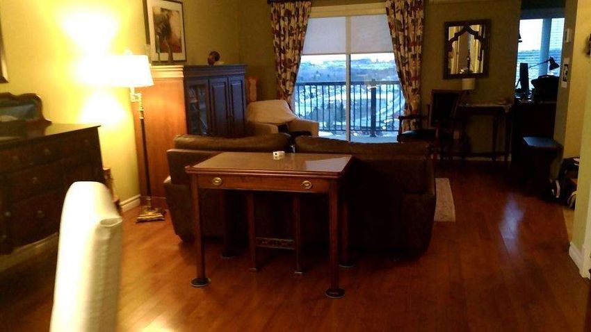
TABLE I
 C UMULATIVE LOCALIZATION PERFORMANCE (%) AND AVERAGE LOCALIZATION JUMPS ( MM ) OF THE SIX LOCALIZATION SESSIONS ON EACH MAP
                                                          FOR EACH VISUAL FEATURE USED .

                           Localization (%)                               Visual Inliers (%)                      Jumps (mm)
          Map         SU SI BF BK KA FR DY                    SP   SU   SI BF BK KA FR DY          SP    SU   SI BF BK KA FR          DY   SP
          1           67 65 65 58 65 51 66                    87   11   10 15 10 12 14 11          19    56   52 49 57 52 50          45   44
          2           74 69 70 64 69 54 74                    89   11   10 14 10 12 13 10          19    40   38 41 47 45 42          36   37
          3           86 82 85 79 81 70 86                    95   13   11 16 11 15 15 13          23    42   45 45 46 47 44          41   35
          4           89 84 87 83 84 76 88                    96   13   12 16 11 15 15 13          24    38   48 43 45 45 42          36   33
          5           79 76 79 71 74 65 79                    91   13   12 16 12 15 16 13          22    40   46 45 51 46 46          39   32
          6           76 74 74 67 72 62 76                    90   13   12 17 12 16 17 13          21    42   47 40 52 41 48          39   36
          1+6         94 91 91 87 90 84 90                    97   14   13 18 12 17 16 14          25    35   38 40 44 38 40          36   29
          1+3+5       97 95 96 94 95 91 97                    99   16   14 18 13 18 18 16          27    32   33 39 42 37 39          31   28
          2+4+6       98 95 96 93 95 91 97                    98   16   14 19 13 18 18 16          27    31   37 35 37 38 35          30   27
          1+2+3+4+5+6 99 98 99 98 97 95 99                    99   18   16 20 15 20 20 18          29    26   30 33 39 29 31          26   25
          1|2|3|4|5|6 97 95 96 96 94 92 96                    98   17   14 19 14 19 18 16          27    28   30 31 36 31 32          27   27

                        TABLE II
                                                                                  Robotics and Automation, 2013.
  RAM USAGE (MB) COMPUTED WITH VALGRIND ’ S M ASSIF TOOL OF                  [13] C. Valgren and A. J. Lilienthal, “SIFT, SURF and seasons: Long-
             EACH MAP FOR EACH VISUAL FEATURE USED .                              term outdoor localization using local features,” in 3rd European Conf.
                                                                                  Mobile Robots, 2007, pp. 253–258.
Map                      SU      SI   BF    BK    KA    FR     DY     SP     [14] N. Carlevaris-Bianco and R. M. Eustice, “Learning visual feature
                                                                                  descriptors for dynamic lighting conditions,” in IEEE/RSJ Int. Conf.
1 (206 nodes)            113    177    64    80    99    68    233    213         Intelligent Robots and Systems, 2014, pp. 2769–2776.
2 (205 nodes)            110    171    63    79    90    66    227    196    [15] D. DeTone, T. Malisiewicz, and A. Rabinovich, “Superpoint: Self-
3 (210 nodes)            112    174    64    80    95    67    232    202         supervised interest point detection and description,” in Proc. IEEE
                                                                                  Conf. Computer Vision and Pattern Recognition Workshops, 2018, pp.
4 (193 nodes)            102    159    60    74    87    62    211    190         224–236.
5 (176 nodes)             92    142    55    66    78    56    189    167    [16] M. Labbé and F. Michaud, “RTAB-Map as an open-source lidar
6 (240 nodes)            120    185    71    86   104    72    251    208         and visual simultaneous localization and mapping library for
                                                                                  large-scale and long-term online operation,” J. Field Robotics,
1+6                      237    365   135   168   206   140    486    423         vol. 36, no. 2, pp. 416–446, 2019. [Online]. Available: https:
1+3+5                    320    490   182   225   272   190    648    569         //onlinelibrary.wiley.com/doi/abs/10.1002/rob.21831
2+4+6                    338    516   195   240   284   200    685    587    [17] G. Grisetti, R. Kümmerle, C. Stachniss, and W. Burgard, “A tutorial
                                                                                  on graph-based SLAM,” IEEE Intelligent Transportation Systems
1+2+3+4+5+6              675   1015   382   468   566   393   1319   1150         Magazine, vol. 2, no. 4, pp. 31–43, 2010.
Constant Overhead         90     90    90   225    90    90    155   1445    [18] F. Dellaert, “Factor graphs and GTSAM: A hands-on introduction,”
                                                                                  Georgia Institute of Technology, Tech. Rep., 2012.
                         TABLE III                                           [19] G. Bradski and A. Kaehler, Learning OpenCV: Computer Vision with
                                                                                  the OpenCV Library. O’Reilly Media, Inc., 2008.
  AVERAGE LOCALIZATION TIME AND WORDS PER FRAME FOR EACH                     [20] M. Calonder, V. Lepetit, C. Strecha, and P. Fua, “Brief: Binary robust
  VISUAL FEATURE USED , ALONG WITH DESCRIPTOR DIMENSION AND                       independent elementary features,” in European Conf. Computer Vision.
        NUMBER OF BYTES PER ELEMENT IN THE DESCRIPTOR .
                                                                                  Springer, 2010, pp. 778–792.
                                                                             [21] S. Leutenegger, M. Chli, and R. Y. Siegwart, “BRISK: Binary robust
                                                                                  invariant scalable keypoints,” in IEEE Int. Conf. Computer Vision,
                   SU        SI BF     BK KA FR         DY SP                     2011, pp. 2548–2555.
        Time (ms) 87        203 67     148 449 92       152 353              [22] P. F. Alcantarilla, A. Bartoli, and A. J. Davison, “Kaze features,” in
        Words     847       770 889    939 640 580      847 472                   European Conference on Computer Vision. Springer, 2012, pp. 214–
                                                                                  227.
        Dimension 64        128 32      64 64 64        200 256              [23] A. Alahi, R. Ortiz, and P. Vandergheynst, “Freak: Fast retina keypoint,”
        Bytes/Elem 4         4 1        1 4 1            4 4                      in IEEE Conf. Computer Vision and Pattern Recognition, 2012, pp.
                                                                                  510–517.
                                                                             [24] E. Tola, V. Lepetit, and P. Fua, “Daisy: An efficient dense descriptor
                                                                                  applied to wide-baseline stereo,” IEEE Trans. Pattern Analysis and
 [8] P. Corke, R. Paul, W. Churchill, and P. Newman, “Dealing with shad-          Machine Intelligence, vol. 32, no. 5, pp. 815–830, 2009.
     ows: Capturing intrinsic scene appearance for image-based outdoor       [25] M. Muja and D. G. Lowe, “Fast approximate nearest neighbors with
     localisation,” in IEEE/RSJ Int. Conf. Intelligent Robots and Systems,        automatic algorithm configuration,” in Proc. Int. Conf. Computer
     2013, pp. 2085–2092.                                                         Vision Theory and Application, 2009, pp. 331–340.
 [9] S. M. Lowry, M. J. Milford, and G. F. Wyeth, “Transforming morning      [26] M. Labbé and F. Michaud, “Long-term online multi-session graph-
     to afternoon using linear regression techniques,” in IEEE Int. Conf.         based splam with memory management,” Autonomous Robots, Nov
     Robotics and Automation, 2014, pp. 3950–3955.                                2017.
[10] D. G. Lowe, “Distinctive image features from scale-invariant key-       [27] R. Kummerle, G. Grisetti, H. Strasdat, K. Konolige, and W. Burgard,
     points,” Int. J. Computer Vision, vol. 60, no. 2, pp. 91–110, 2004.          “g2o: A general framework for graph optimization,” in IEEE Int. Conf.
[11] H. Bay, A. Ess, T. Tuytelaars, and L. V. Gool, “Speeded Up Robust            Robotics and Automation, May 2011, pp. 3607–3613.
     Features (SURF),” Computer Vision and Image Understanding, vol.         [28] X. Shi, D. Li, P. Zhao, Q. Tian, Y. Tian, Q. Long, C. Zhu, J. Song,
     110, no. 3, pp. 346–359, 2008.                                               F. Qiao, L. Song, et al., “Are we ready for service robots? The
[12] P. Ross, A. English, D. Ball, B. Upcroft, G. Wyeth, and P. Corke,            OpenLORIS-scene datasets for lifelong SLAM,” in IEEE Int. Conf.
     “A novel method for analysing lighting variance,” in Australian Conf.        Robotics and Automation, 2020, pp. 3139–3145.
You can also read