Contributions from Eric Greenwood NASA Langley Research Center!
←
→
Page content transcription
If your browser does not render page correctly, please read the page content below
Matt
  Johnson

           Robert
  Morris

                                                                  IHMC,
  USA

 NASA
  Ames
  Research

  Center,USA


          K.
  Brent
  Venable
                        James
  Lindsey

Tulane
  University
  and
  IHMC,USA
            Monterey
  Technologies,
  USA


           Contributions
  from
  Eric Greenwood NASA Langley Research Center!
Motivation
and
Objectives
Technical
Background
Rotorcraft
Noise
and
Noise
Simulation
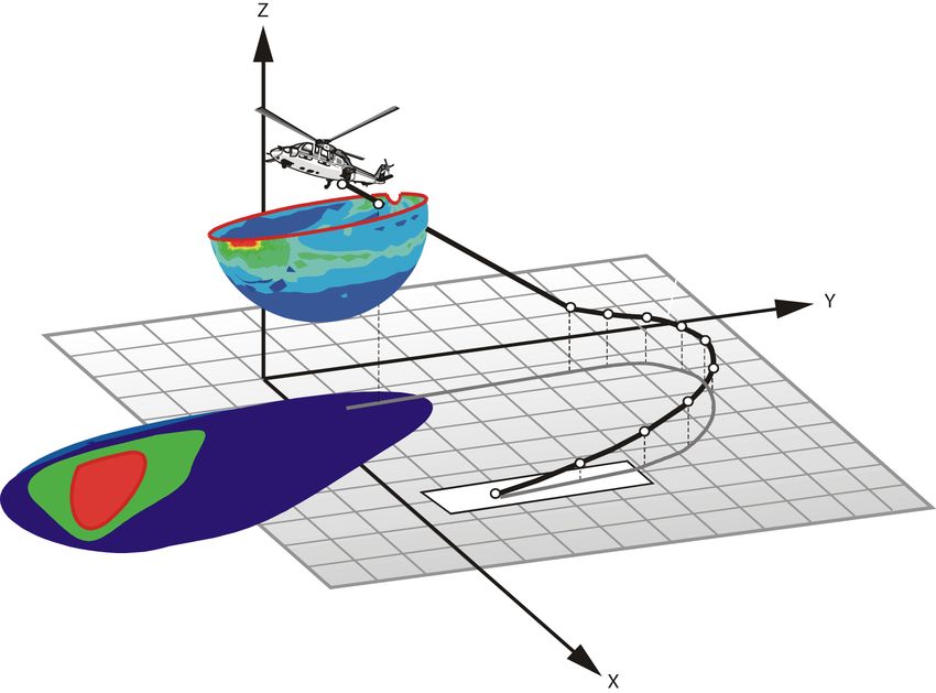
Trajectory
Optimization
Summary
of
Approach
Constraint
Model
Cost
Function
Search
Experiments
Summary
and
Future
Work
March
26,
2013
IWPSS
2013
¡ Promote
the
use
of
rotorcrafts
for
commercial
transportation
¡ Apply
state
of
the
art
AI
techniques
to
design
rotorcraft
approach
trajectories
that
minimize
ground
noise.
¡ Why
AI?
§ Difficult
for
pilots
to
predict
accurately
the
impact
of
their
decisions
on
noise
§ Too
many
variables:
helicopter
model,
BVI,
ground
conformation,
wind,
comfort
¡ Use
robust
noise
predictor
to
evaluate
candidate
trajectories
§ Prediction
used
to
define
cost
function.
¡ Noise
is
“unwanted
sound”
§ A
subjective
quantity
¡ Sound
is
any
pressure
variation
a
human
ear
can
detect
§ An
objective
quantity
¡
The
decibel
scale
matches
the
way
our
ear
and
brain
“auditory
system”
interprets
sound
pressures
§ We
“hear”
in
decibels.
¡ Sound
Exposure
Level
(SEL)
is
a
measure
of
the
total
“noisiness”
of
an
event,
that
takes
duration
into
account
§ FAA
considers
a
1.5
dB
the
minimum
significant
change
¡ Rotorcraft
tend
to
have
strong
impulsive
and
directional
characteristics
compared
to
fixed
wing
aircraft.
¡ Noise
levels
can
vary
significantly
depending
on
vehicle
design
and
flight
condition.
¡ For
low
speed
descent,
where
Blade
Vortex
Interaction
(BVI)
noise
may
be
present,
noise
levels
can
be
10-‐20dB
higher
than
for
flight
conditions
where
BVI
noise
is
not
present.
¡ Propagation
effects
of
source
noise
dependent
on
atmospheric
and
terrain
conditions.
¡ Therefore,
characterizing
ground
noise
exposure
is
hard!
March
26,
2013
IWPSS
2013

• Main
rotor
• Tail
rotor
• Engine
• Drive
system
• Blade
Vortex
Interaction
(BVI):
modulation
of
sound
by
the
relatively
slow-‐turning
main
rotor.
• Happens
when
one
blade
interacts
with
the
vortex
of
the
previous
blade.
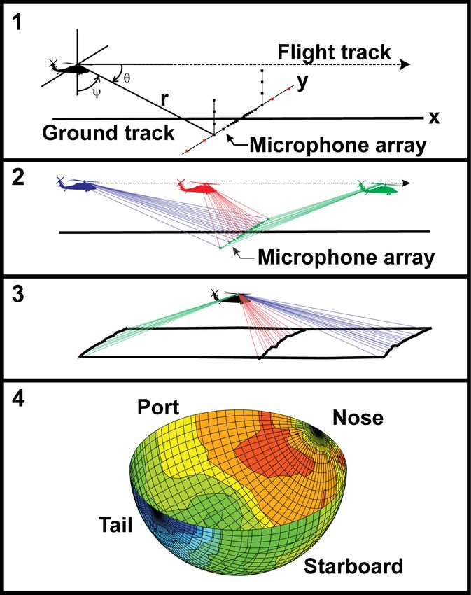
¡ RNM
is
a
simulation
program
that
§ models
sound
propagation
through
the
atmosphere
§ predicts
noise
levels
on
flat
ground
or
varying
terrain.
¡ Purpose
§ Aid
assessment
of
low
noise
terminal
area
operation
procedures
for
rotorcrafts;
§ Improve
rotorcraft
modeling
capabilities
DIAGNOSTICS
Example
of
RNM
Input
parameters:
COMPUTEPOI
COMPUTEPLT
input
file
¡ Identity
of
the
rotorcraft
QSAM1
¡ Dimension
and
resolution
of
SETUP
PARA
200
200
500
a
grid
(region
of
interest)
-‐1000
-‐1000
5
¡ Particular
points
of
interest
3000
1000
(if
desired)
60
30000
10000
0.0
CH146
¡ A
flight
trajectory
(3D
1
location,
velocity
and
0.00
0.00
0.00
orientation)
0
0
ONE
TRACK
rnmAnalysis
2
0.0
0.0
1249.3280028431807
0.00
0.00
90.0
0.00
0.00
0.00
90.0
2000.0
0.0
750.6719971568193
0.00
0.00
90.0
0.00
0.00
0.00
90.0
END
•   Sound
  is
  analytically
  propagated
  through


    the
  atmosphere
  to
  the
  ground.


•   RNM
  currently
  accounts
  for

    • Spherical
  spreading

    • Atmospheric
  absorption

    • Ground
  reflection
  and
  attenuation

    • Doppler
  shifts

    • Different
  ground
  terrains

    • Effects
  of
  wind
  and
  temperature

    • Multiple
  noise
  sources
  (main
  rotor,
  tail

      rotor,
  engine,
  etc.)


•   RNM
  produces
  contour
  plots:
  graphical

    representation
  of
  ground
  noise
  exposure

    using
  a
  number
  of
  noise
  metrics
  over
  the

    designated
  grid

                                                                        SEL
  values
*courtesy
E.
Greenwood
¡ RNMs
prediction
are
based
on
sound
hemispheres
summarizing
test
results
¡ Helicopter
maintains
steady
flight
condition
throughout
measurement
¡ Observation
angles
of
microphones
shift
during
flyover
¡ Single
“compact”
source
of
emission
assumed
(typically
main
rotor
hub)
¡ Measurements
resolved
to
surface
of
hemisphere
*courtesy
  E.
  Greenwood


          If an exact match for a desired flight segment is not !
          found in the database of hemispheres, a new !
     hemisphere is generated by interpolating the noise levels !
on the surface of the hemisphere between known values!
of airspeed and flight path angle.!
¡ Data
resolution
is
the
distance
between
any
two
grid
points
¡ RNM
predicts
ground
noise
at
each
point
¡ Higher
resolution
means
§ more
accurate
predictions,
but
§ longer
computation
time
March
26,
2013
IWPSS
2013
Performance/Resolution
  Tradeoff

                                                                   Time (sec)

            1400

            1200

            1000

              800
                                                                                              Time (sec)
              600

              400

              200

                    0
                            0   200            400           600        800     1000   1200
                                                          Resolution

 March
  26,
  2013
               IWPSS
  2013
¡ Problem
is
to
find
a
sequence
of
control
actions
for
that
minimizes
a
performance
function.
▪ Example
performance
functions
pertain
to
time,
radar
exposure,
fuel,
and
noise.
¡ System
dynamics
are
described
by
▪ Variables
z
=[y,u],
where
y
are
state
variables
and
u
are
control
variables.
▪ State
equations
Á
=
f(y(t),u(t),t)
describing
the
dynamics
of
the
system.
▪ Initial
and
terminal
conditions.
▪ Bounding
constraints
on
state
and
control
variables.
¡ Standard
approaches
for
solving
trajectory
optimization
problems
are
based
either
on
methods
of
optimal
control
or
on
approximations
to
optimal
control
based
on
non-‐linear
programming
¡ Recently,
sample
methods
have
evolved
as
the
optimizers
of
choice
March
26,
2013
IWPSS
2013
¡ Discrete
optimization
approach
to
planning
involving
grids.
¡ Vehicle
model
of
position
and
attitude
¡ State
transition
model
that
incorporates
constraints
on
safety
and
comfort.
¡ Noise
cost
function
that
aggregates
data
from
RNM
¡ Discretization
of
search
space
for
allowing
solutions
at
different
resolutions
¡ Empirical
comparison
of
A*
with
Stochastic
Local
Search
March
26,
2013
IWPSS
2013
¡State
space
is
a
grid
of
points
in
3D
space.
¡Action
space
is
2D
grid
of
changes
in
velocity
or
altitude
¡Limits
imposed
by
constraints
on
deceleration
and
rate
of
descent.
¡A
solution
trajectory
is
a
sequence
of
state
and
action
pairs
¡Single
start
and
end
state.
17
March
26,
2013
IWPSS
2013
•For
the
experiments,
we
fixed
the
x-‐y
values
to
conform
to
standard
approach.
•Result
is
trajectory
optimization
problem
in
2
dimensions
(deceleration
and
descent)
March
26,
2013
IWPSS
2013
n1
X
w1
125-‐db
+
n2
X
w2
101,124db
+
n3
X
w3
75,100db
+
n4
X
w4
0,75db
• Based
  on
  two
  independent
  sets
  of

          experiments
  associating
  dB
  levels

          with
  annoyance.


•


•Weights
  were
  based
  on
  curve
  in

graph.
• Separate
search
and
evaluation
phase
§ Search
phase
uses
either
A*
or
SLS
to
generate
solution
¡ Evaluation
phase
consists
of
run
of
RNM
and
evaluation
using
BIN
cost
function.
¡ Local
Stochastic
Search
§ Allows
for
large
exploration
of
search
space
with
little
knowledge
of
what
is
being
optimized
Traj.
RNM
¡ Uses
RNM
as
evaluator
of
candidate
solutions
¡ Randomly
generated
initial
solutions
Optimizer
Y
Cost
¡ Cost
functions
based
on
Function
aggregation
of
predicted
noise
levels
Given an optimization problem and the
              search space of its solutions, start from an
              initial start position and improve iteratively
              by means of minor modification

                                                       neighborhood

                          solution space              current solution
solution quality

local optimum¡Search space: all possible “box” landing trajectories Suggested by pilot as typical approaches A trajectory is a sequence of state-‐action pairs called nodes ¡Neighborhood of a box trajectory T: Set of trajectories obtained from T by picking any two nodes and transferring quantities of deceleration or decent from one to the other
Δv
or
Δz
Neighbor
Current
trajectory
δz
δv
i-‐1
i
i+1
Di=(Δvi,Δzi)
Di-‐1=(Δvi-‐1,Δzi-‐1)
Di+1=(Δvi+1,Δzi+1)
Si=(xi,yi,vi,zi)
Si-‐1=(xi-‐1,yi-‐1,vi-‐1,zi-‐1)
Si+1=(xi+1,yi+1,vi+1,zi+1)
March
26,
2013
IWPSS
2013
Δv
  or
  Δz

                                             Neighbor


  Current
  trajectory
                                   RNM


                        Scalar
  Cost

                        Function


Score
Current
solution
Neighbor
Score=
number
of
points
where
neighbor
is
significantly
more
quiet
–
number
of
points
where
it
is
significantly
more
loud
Significantly
à
≥1.5 dB
•Complete
best-‐first
search
algorithm
based
on
incremental
expansion
of
solution
guided
by
heuristic
d
estimation
function.
waypoint
V
•
Heuristic
estimate
of
cost-‐to-‐go:
fly
high
and
slow
to
s
goal.
d
•Flying
slow
to
goal
state
without
descending
Z
•Empirically
shown
to
be
admissible
•Aggregating
cost
is
problematic
because
noise
of
path
is
not
a
simple
aggregation
of
path
segments.
March
26,
2013
IWPSS
2013
¡ Conditions that make a trajectory suitable to fly !
§ Angle of descent between 0 and 12 degrees!
§ Deceleration between 0 and 0.1 gs!
¡ A trajectory is flyable if it satisfies all the
deceleration and angle-of-decent constraints
along its path.!
¡ Enforced by neighborhood function!¡ Primary goal is to demonstrate potential for
improvements to standard approaches followed
by pilots!
§ Provide inputs to acoustic field tests!
§ Comparison of solutions with ’standard operations’!
¡ Comparisons of A* with SLS with respect to:!
§ Quality and run time performance!
§ Effects of varying grid resolution !
March
26,
2013
IWPSS
2013
¡ SLS
algorithm
has
tunable
parameters
to
adjust
the
§ randomness
of
search
§ depth
of
search
¡ Additional
parameters
are
used
to
adjust
§ Grid
resolution
(number
of
data
points)
§ Search
resolution
(number
of
control
actions)
March
26,
2013
IWPSS
2013
Low
  Search
  Res


High
  Search
  Res
Low
  Grid
  Res


High
  Grid
  Res
AI-‐suggested
Path
Pilot-‐suggested
Path
velocity
velocity
altitude
altitude
Feet
to
landing
point
Feet
to
landing
point
¡ Rapidly-‐exploring
Random
Trees
¡ Probabilistic
Road
Maps:
1. Sampling
1
§ 4-‐d
space
(x,y,z,v,h)
with
heading
2. Linking
§ Flyability
constraints
3. Weighting
§ Bin
function
score
4. Shortest
Path
2
¡ Running
RNM
is
the
heaviest
part
of
computation
¡ Bypass
RNM
with
an
ML-‐based
surrogate
that
will
predict
the
value
of
the
cost
function
¡ Imported
GIS
data
¡ Weight
contour
plots
according
to
land
usage
March
26,
2013
IWPSS
2013
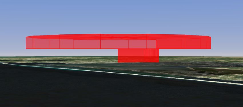
¡ Incorporate
airspace
constraints,
such
as
Class
C
airspace
and
approach
corridors
for
active
runways
Top View
Side
View
March
26,
2013
IWPSS
2013
¡ Fixed
seed
§ Starts
from
a
fixed
trajectory
suggested
by
pilots
§ Picks
random
neighbor
if
neighborhood
is
empty
¡ Random
seed
§ Starts
from
a
fixed
trajectory
suggested
by
pilots
§ Picks
random
trajectory
if
neighborhood
is
empty
¡ 50-‐50
§ Random
start
§ 50%
of
the
time
picks
a
random
solution
¡ Runtime
behavior,
average
on
200
runs
¡ Path
Planning
techniques
¡ A*
dV
waypoints
dZ
Michele
  Donini

                            Jim
  Lindsey


 Robert
  Morris


                                                                          Marco
  Pegoraro


Matt
  Johnson


                                                                          Riccardo
  Tesselli


                                                 Riccardo
  Ferro

  Tom
  Eskridge
     Daniel
  Duran
You can also read