CourtVision: New Visual and Spatial Analytics for the NBA
←
→
Page content transcription
If your browser does not render page correctly, please read the page content below
CourtVision: New Visual and Spatial Analytics for the NBA
                                          Kirk Goldsberry, Ph.D.
                                            Harvard University,
                                 1730 Cambridge St, Cambridge, MA, 02138
                                    Email: kgoldsberry@fas.harvard.edu

                                                 Abstract
     This paper investigates spatial and visual analytics as means to enhance basketball expertise. We
     introduce CourtVision, a new ensemble of analytical techniques designed to quantify, visualize, and
     communicate spatial aspects of NBA performance with unprecedented precision and clarity. We propose
     a new way to quantify the shooting range of NBA players and present original methods that measure,
     chart, and reveal differences in NBA players’ shooting abilities. We conduct a case study, which applies
     these methods to 1) inspect spatially aware shot site performances for every player in the NBA, and 2) to
     determine which players exhibit the most potent spatial shooting behaviors. We present evidence that
     Steve Nash and Ray Allen have the best shooting range in the NBA. We conclude by suggesting that
     visual and spatial analysis represent vital new methodologies for NBA analysts.

1 Introduction
          Basketball is a spatial sport; the structure and dynamics of “court space” influence every instant of every
basketball game, yet very few contemporary statistical or evaluative approaches account for spatial components.
Whether it’s the nuances of shot site selection, defensive schemes, or player spacing, basketball expertise requires
spatial reasoning. Although every player and every team in the NBA exhibits unique spatial behaviors, current
analytics fail to effectively capture these crucial differences. As the NBA becomes more analytically driven, there is
an emerging need for spatially informed evaluations that can be effectively communicated to a diverse set of
audiences; enhanced spatial and visual analytics could be vital new tools for informing future game plans, personnel
transactions, and practice regimens. In this paper, we introduce “CourtVision,” a new ensemble of spatial and visual
analytics designed to reveal, quantify, visualize, and communicate on-court performance with unprecedented
precision and clarity. We present new spatial metrics and advanced visualizations that enable organizations to better
understand the complex spatial dynamics of NBA players and teams.

          CourtVision integrates database science, spatial analysis, and visualization to reveal players’ and teams’
unique spatial signatures; in turn, these signatures expose important patterns and anomalies in performance that are
considerably less evident using conventional evaluative approaches. The results facilitate efficient answers to
important questions about the NBA such as: Where are players’ most common shot locations and how successful
are they at these locations? Which point guard has the highest points per attempt at the top of the key? Which court
locations are most or least effectively defended by the Orlando Magic? The answers to these kinds of questions hold
obvious strategic advantages, but to this point few analytical techniques provide them.

          The long-term goals of our research are 1) to advance basketball expertise with new spatial and visual
analytics that reveal key space-based variation in player and team performances, 2) to develop new player- and team-
based spatial metrics that quantify the associations between court space and performance, 3) to design and
implement new spatially-aware models that predict which players and offensive teams will perform best and worst
against which team defenses and 4) to translate these results into forms effectively communicated amongst diverse
audiences. In this paper, our specific aims are to 1) introduce spatial limitations of contemporary shooting metrics,
2) identify key spatial variables of NBA shooting performances that remain misunderstood, and 3) demonstrate how
visual analytics and spatial analysis can expose differences in shooting behavior. We present a league-wide case study
that attempts to answer one simple yet complex question: who is the best shooter in the NBA?

2 Background

          The inability of conventional basketball evaluation to reveal spatial differences hinders the ability of NBA
analysts to fully uncover or communicate key on-court performance variables that shape competitive outcomes. For
example, current approaches fail to effectively reveal players’ and teams’ unique spatial shooting tendencies; this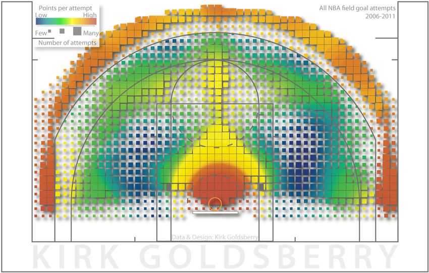
MIT Sloan Sports Analytics Conference 2012
                                                                         March 2-3, 2012, Boston, MA, USA

means that 1) key NBA scoring phenomena remain misunderstood, and 2) there is an opportunity to synthesize
emerging techniques from spatial analysis and visual analytics to enhance our understanding of NBA shooting.

          The most commonly used NBA shooting metrics, including field goal percentage (FG%) do not account
for spatiality. Although conventional metrics are simple ways to summarize the probability of a shot attempt
resulting in a made basket they fail to expose true differences in shooting ability across the league. For example,
according to FG%, the most effective shooter in the NBA in 2010-2011 season was Nene Hilario, who posted a
61.5% FG%. In fact every player who ranked within the top 10 in FG% in 2010-2011 was a forward or a center; no
guards, who are generally regarded as the game’s best shooters, made the list. Enhanced Field Goal Percentage or
eFG% attempts to mitigate this issue by controlling for the differing value between a three point and two point field
goal but still fails to differentiate between different kinds of 2 point and 3 point field goals.

          Spatial analysis and visual analytics can greatly enhance shooting evaluations. Spatial analysis, originally
called “spatial data analysis”[1] is an extension of conventional statistics that supports the analysis of spatial variation
and enables analysts to describe the distribution of phenomena in space, visualize the spatial patterns of phenomena,
and quantify/compare spatial relationships amongst various phenomena[2,3]. With potent applications in Ecology,
Public Health, Military Science, and many other disciplines, spatial analysis is a rapidly growing field. However,
despite the fact that every player and team in the NBA exhibits unique spatial behaviors, with the exception of a few
small, targeted studies[4,5,6] hardly any evaluative approaches of basketball include spatial analyses; as a result critical
spatial variance of NBA players and teams remains undetected, and potential competitive advantages are yet to be
realized.

        Many key basketball strategies pertain to understanding the complexity of spatial performances. For
example, some teams might employ a zone defense as a means to more effectively defend certain court spaces.
During the 2010-2011 season the Dallas Mavericks famously used zone defense to augment the spatial behavior of
the Miami Heat:

    “In two regular season games with the Mavs this year, Miami faced a zone defense on 56 offensive
    possessions or about one-fourth of the time. On these plays, the Heat shot 13-of-45 from the field
    (28.9%), resulting in an offensive efficiency of .55 points per possession – both marks are well below their
    season average. Of the 45 shots the Heat attempted in these two games, just 10 were in the paint,
    surprising when considering that a majority of these touches came in isolation and pick-and-roll sets. This
    isn’t to say players like LeBron James and Dwyane Wade aren’t able to penetrate against this zone look, but
    rather the swift rotation of the Dallas frontcourt forces them to kick and settle for perimeter jumpers.”[7]

         In this example, Dallas successfully adapted a strategy to limit access to locations of spatial potency of
Miami. But, how were these locations identified and analyzed? Analytical reasoning about court space in the NBA is
both vital and undeveloped. The spatial terminology in the above passage reveals the coarse nature of the status quo
of place-based reasoning in basketball expertise; the court is commonly divided into only a few imprecise regions
including “the paint,” “the wing,” and the always vague, “perimeter.” Conversely, important performance variations
occur at finer resolutions within these crude regions; analysis in basketball has failed to take advantage of the
advanced spatial data recorded for every NBA game. Conventional analyses are overly coarse, and there is an
opportunity to apply spatial analysis to evaluate game play in a much more precise fashion.

          Throughout their analytical processes, NBA analysts identify and create elements of information that
contribute to reaching defensible strategic judgments[8]; these elements are sometimes called “reasoning artifacts,”
and are designed to be shared with fellow analysts, executives, coaches, and players to communicate performance
issues. In other spatial strategy domains such as emergency management, homeland security, and public health,
graphical reasoning devices such as maps, diagrams and other well-designed visual artifacts enable analysts to not
only identify key spatial insights, but also to effectively communicate them amongst diverse audiences - there is a
similar prospect for the NBA that remains unrealized.

          Visual Analytics is an evolving field that empowers new insights and analytical reasoning via graphical
representations of complex information. As the NBA becomes more “data-rich,” and its analysts seek novel ways to
understand and communicate performance phenomena, there is a need for techniques that translate raw game data
into clear and useful information; we contend that visual analytics present one potent, overlooked solution to this
problem. Visual analytics strives to facilitate the analytical reasoning process via graphical data interfaces (e.g. maps
and diagrams) that maximize human capacity to perceive, understand, and reason about complex and dynamic data
and situations[8]. Overall, the goal of visual analytics is to empower effective human judgment with a limited
investment of the analysts’ time. Since NBA Analysts commonly reach complex strategic spatial judgments under

                                                             2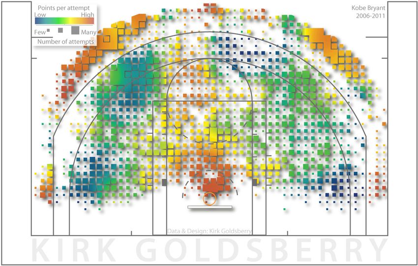
MIT Sloan Sports Analytics Conference 2012
March 2-3, 2012, Boston, MA, USA
significant time pressure there is a need for efficient visualizations that streamline connections between spatial game
data, reasoning artifacts, analysts, and other audiences.
3 Case Study: Who is the best shooter in the NBA?
As a means to evaluate the feasibility of spatial and visual analytics for the NBA, we conducted a case study
that attempted to answer one simple question: who is the best shooter in the NBA? Conventional metrics and
evaluative approaches fail to provide a simple answer to this question. For example, Nene Hilario and Dwight
Howard led the league in FG% in the 2010-2011 season, but neither is considered to be a great shooter. What
makes a shooter great? What criteria separate good shooters from bad shooters? When asked who was the best
shooter in the league, NBA reporter David Aldridge suggested it was Ray Allen because of his ability to shoot well
from many different locations on the court: “Everyone has their favorite spots on the court but it seems like Ray
[Allen] is more comfortable in more places than anyone I’ve seen.”
There is a clear spatial criterion implied in Aldridge’s answer; he is implying that all shooters perform better
at some places than others, but great shooters possess the ability to shoot well from many locations on the floor –
the capability to make baskets from several different court locations is commonly referred to as “shooting range.”
Although this seems like a sensible and useful assessment criterion, shooting range has yet to be effectively
quantified and consequently has been mostly neglected in current evaluative approaches. To determine the best
shooters in the NBA, we generated an analytical framework that 1) employs spatial analysis to quantify shooting
range, and 2) visual analytics to reveal the unique spatial tendencies of individual shooters. Below, we describe the
case study’s data, methods, and results.
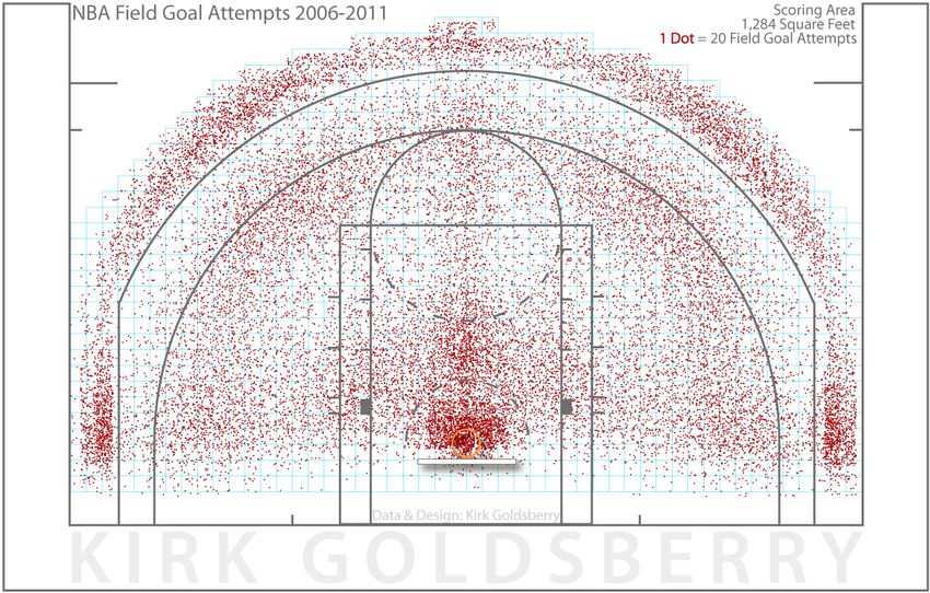
Data: Using game data sets for every NBA game played between 2006 and 2011, we compiled a spatial
field goal database that included Cartesian coordinates (x,y) for every field goal attempted in this 5-year period. This
data set includes player name, shot location, and shot outcome for over 700,000 field goal attempts. We mapped the
shot data atop a base map of a NBA basketball court (Figure 1). Although a regulation NBA court is 4,700 ft2, (50ft
x 94ft), almost all (>98%) field goal attempts occur within a 1,284 ft2 area in between the baseline and a relatively
thin buffer around the 3-point arc; we call this area the “scoring area.” We divided the scoring area into a grid
consisting of 1,284 unique “shooting cells,” each 1 ft2 (Figure 1). To quantify shooting range, we applied spatial
analyses to evaluate shooting performance across the grid and within each shooting cell.
Figure 1: Our composite shot maps from 2006-2011 NBA game data. The map on the left summarizes the density of all field
goal attempts during the study period. The map on the right reveals league-wide tendencies in both shot attempts and points per
attempt. Larger squares indicate areas where many field goals were attempted; smaller squares indicate fewer attempts. The color
of the squares is determined by a spectral color scheme and indicates the average points per attempt for each location. Orange
areas indicate areas where more points result from an average attempt, and blue areas indicate fewer points per attempt.
We derived metrics that described spatial aspects of shooting performance throughout the scoring area.
The most basic metric is called “Spread,” which is simply a count of the unique shooting cells in which a player has
attempted at least one field goal. The raw result is a number between 0 and 1,284 and summarizes the spatial
diversity of a player’s shooting attempts. By dividing this count by 1,284 and multiplying by 100, we generated
Spread%, which indicates the percentage of the scoring area in which a player has attempted at least one field goal.
Spread = ∑ FGAij
ij ∈SA
Spread = Total spatial spread of player across all scoring cells
FGAij = 1, if at least one field goal has been attempted in cell i, 0 if not
SA = Scoring area consisting of 1,284 scoring cells
€
3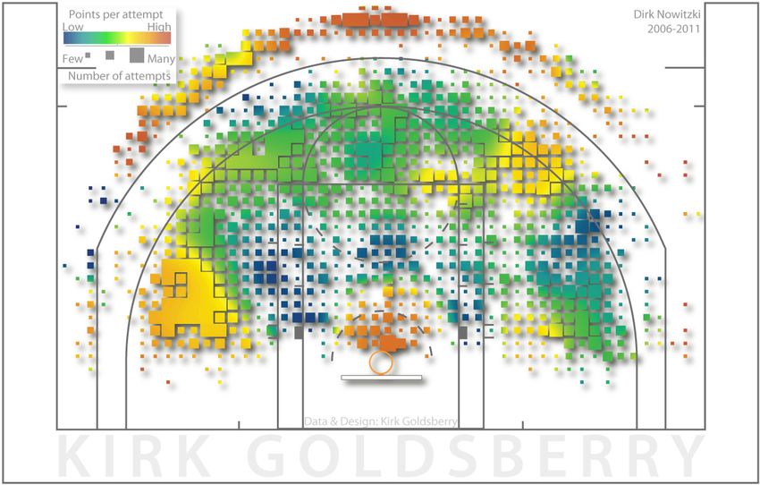
MIT Sloan Sports Analytics Conference 2012
                                                                             March 2-3, 2012, Boston, MA, USA

          Spread describes the overall size of a player’s shooting territory. League leaders in FG% generally have a
small Spread value since they tend to only shoot near the basket. For example, since centers generally thrive in
limited areas near the hoop they tend to have lower Spread values than shooting guards. Kobe Bryant has the
highest spread value in the NBA (table 1); Bryant’s value of 1,071 indicates he has attempted field goals in 1,071 of
the 1,284 shooting cells or 83.4% of the scoring area. In contrast, Dwight Howard has attempted field goals in only
23.8% of the shooting cells. Although Spread% favors players who simply shoot frequently, it also reveals that some
players like Dwight Howard who do shoot a lot, only do so in limited court spaces. For example, Al Jefferson
attempted 400 more field goals than Ray Allen during the study period, yet his Spread value is only 595 (46.3%),
while Ray Allen’s is 952 (74.1%). Visual depictions of the spread variable expose the stark differences in individual
players’ spatial shooting behaviors. Via the graduated symbol cartographic technique, figure 2 reveals the spatial
structure of Al Jefferson and Ray Allen’s field goal attempts during the study period. Jefferson is highly active in the
central areas near the basket, and clearly favors posting up defenders on the right side of the court. Meanwhile, Ray
Allen is highly active behind the 3-point arc; he attempts many 3-point field goals, but is relatively inactive from
mid-range areas.

Figure 2: Visual depictions of the Spread variable for Al Jefferson and Ray Allen.

          These Spread visualizations reveal a player’s basic shooting tendencies, but tell us nothing about potency.
Shooting skill requires more than just attempts; the best shooters in the league are able to make baskets at effective
rates from many court locations. To describe the spatial potency of players we created a metric called “Range,”
which is a count of the number of unique shooting cells in which a player averages at least 1 point per attempt
(PPA). PPA varies considerably around the court. As anyone who has ever shot a basketball knows, the probability
of a shot attempt resulting in a made basket is spatially dependent; some shots are easier than others, and some
players are unable to shot effectively from most court locations. Range accounts for spatial influences on shooting
effectiveness. It is essentially a count of the number of shooting cells in which a player averages more than 1 PPA;
we chose PPA over FG% because it inherently accounts for the differences between 2-point and 3-point field goal
attempts.

                                                       Range =    ∑ PPAij
                                                                 ij ∈SA
           Range = Effective shooting range of player across all scoring cells
           PPAij = 1, if points per attempt is > 1 in cell i, 0 if not
           SA = Scoring area consisting of 1,284 scoring cells
                                         €
           By dividing this count by 1,284 and multiplying by 100, we generated Range%, which indicates the
percentage of the scoring area in which a player averages more than 1 PPA. Steve Nash is ranked first. He has a
Range value of 406, indicating that he averages over 1 PPA from 406 unique shooting cells, or 31.6% of the scoring
area. Ray Allen was ranked second (30.1%), Kobe Bryant (29.8%) was third, and Dirk Nowitzki (29.0%) was fourth
(table 2). Figure 3 visualizes the shooting range of these four players.

          Steve Nash has the highest Range% in our case study, but does this mean he is the best shooter in the
NBA? That obviously remains debatable; however it is certain that over the last few NBA seasons, Nash and Ray
Allen are the most effective shooters from the most diverse court locations. The average shooter in the NBA has a
Range% of 18.5, meaning they score efficiently from 18.5% of the scoring area. Nash and Allen are the only two
players in the league whose Range% values exceed 30%; only a handful of players in the league average more than 1
PPA from at least 25% of the scoring zone (table 2), and unsurprisingly, despite being among the leaders in FG%,
Dwight Howard (Range% = 6.5) and Nene Hilario (Range% = 3.7) are not on that list. Whether the Range% metric

                                                                 4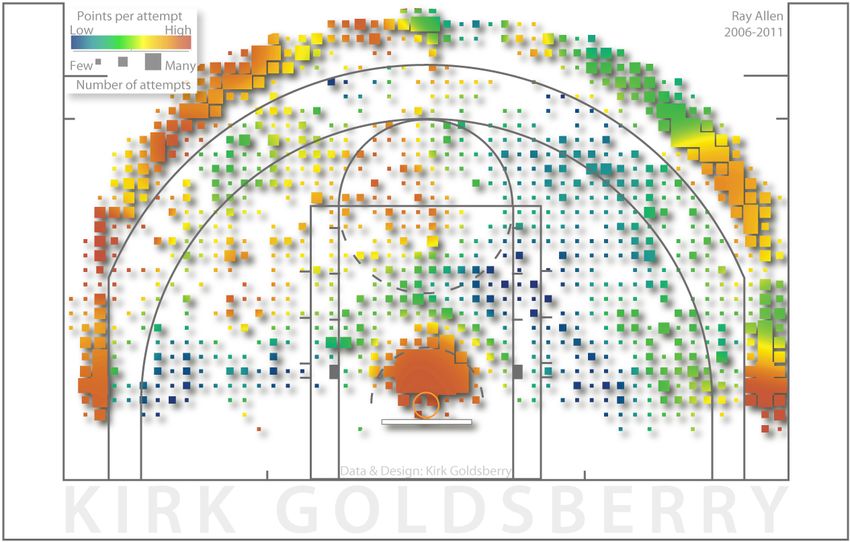
MIT Sloan Sports Analytics Conference 2012
                                                                           March 2-3, 2012, Boston, MA, USA

is the best way of quantifying shooting range or not, it seems to capture pure shooting ability better than FG% or
eFG%.

           Player         Spread      %                                                      Player         Range     %
 1. Kobe Bryant              1,071 83.4%                                            1. Steve Nash              406 31.6%
 2. Lebron James             1,047 81.5%                                            2. Ray Allen               386 30.1%
 3. Vince Carter             1,005 78.3%                                            3. Kobe Bryant             383 29.8%
 4. Joe Johnson                992 77.3%                                            4. Dirk Nowitzki           373 29.0%
 5. Rudy Gay                   983 76.6%                                            5. Rashard Lewis           354 27.6%
 6. Antawn Jamison             965 75.2%                                            6. Joe Johnson             352 27.4%
 7. Andre Igudola              962 74.9%                                            7. Vince Carter            343 26.7%
 8. Ray Allen                  952 74.1%                                            8. Paul Pierce             332 25.9%
 8. Kevin Durant               949 73.9%                                            8. Rudy Gay                332 25.9%
10. Danny Granger              948 73.8%                                           10. Danny Granger           331 25.8%
 Table 1: Top 10 players in Spread metric                                          Table 2: Top 10 players in Range metric

Figure 3: The shooting ranges of Steve Nash, Ray Allen, Dirk Nowitzki, and Kobe Bryant. These four players had the highest
Range values, but these graphics reveal that they achieve them in much different ways. For example, when compared to the three
others, Dirk Nowitzki shoots relatively few 3-point shots and performs much better in the mid-range areas on the left side of the
court, while Ray Allen excels in the corners of the court where Steve Nash rarely shoots.

4 Discussion
           Basketball is a spatial sport. Shooting ability and other performance variables are spatially dependent.
Understanding the spatial dimensions of performance variations is key to basketball expertise. Every coach, player,
fan, scout, and general manager is well aware that the structure and dynamics of court space directly influence every
second of every basketball game. To understand basketball, you need to understand space. In this regard, basketball
is not unique. Spatial reasoning is a primary form of human intelligence that informs everything from tying our
shoes, to launching spacecraft. Visual analytics is an emerging science that focuses on analytical reasoning as
facilitated by intelligent visuals. Graphics including maps, charts, and diagrams are vital tools in every strategic
domain in which space is key; maps inform military campaigns, magnetic resonance imagery informs orthopedic
surgery, and IKEA diagrams enable us to assemble bookshelves. With this in mind, there is a surprising lack of
visual reasoning artifacts used within the basketball community.

                                                               5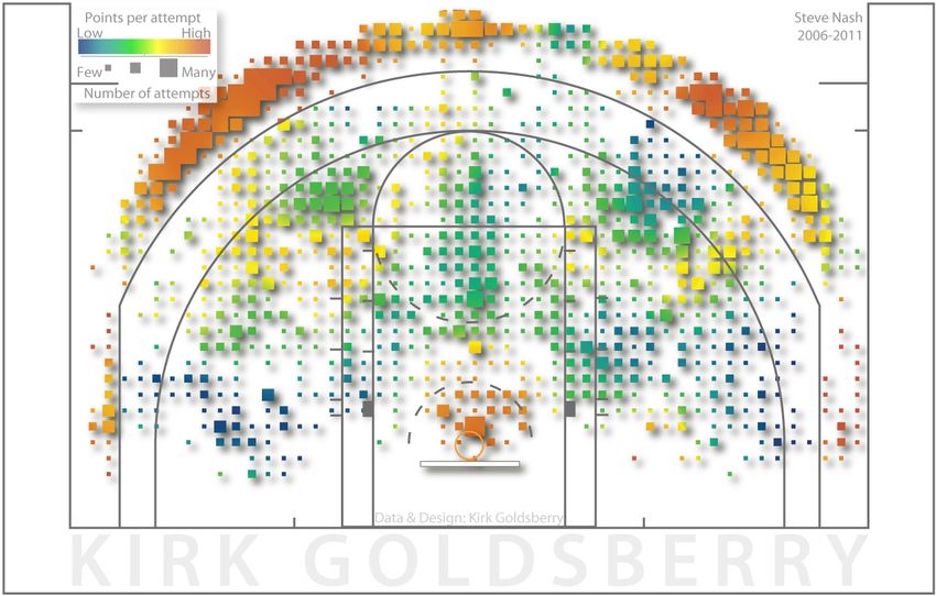
MIT Sloan Sports Analytics Conference 2012
                                                                        March 2-3, 2012, Boston, MA, USA

          Despite a recent proliferation of advanced analytical approaches in basketball[9,10], we have yet to reach a
point where our evaluative approaches sufficiently inform our expertise. Every player and every team in the NBA
exhibits unique spatial behaviors, which shape the competitive outcomes of every minute of every game. The goal of
CourtVision is to reveal these behaviors, quantify them, and communicate them amongst a diverse set of audiences
ranging from analysts, to executives, to scouts, to players. We believe that intelligent basketball graphics can facilitate
unprecedented levels of spatial reasoning and understanding about the sport. We also contend that early adopters of
visual analytics in the NBA may enjoy a competitive advantage over those slow to adopt.

          Although our case study focused on shooting performance, there are several other potential applications of
spatial and visual analytics that can enhance basketball comprehension. Future applications of CourtVision aim to
quantify and visualize spatial variability of other aspects of basketball. For example, the basic ability of a team to
effectively defend court space influences the outcome of every NBA possession. However, some teams and lineups
are more effective defensively than others. Visualizing the spatial signatures of team defenses can reveal strengths
and weaknesses of any team or lineup in the league.

         Similar to shooting, other game events also require further investigation; there are infinite “Where-related”
questions that struggle to be answered by conventional evaluations. For example, where do most steals occur?
Where do most offensive rebounds occur against the Pacers? Where do the Bobcats block most of their shots?
Where on the court does Kevin Garnett commit his personal fouls? Lastly we can combine multiple layers of
performance visualizations to answer complex questions. For example, by overlaying individual players’ shot charts
with team defense charts we can predict which players in the league will perform best and worst against any team
defense. Since some teams defend some places less effectively and certain players excel better from certain locations,
some match-ups are more favorable than others. Basically, every on-court event-type exhibits a unique spatial
signature; every player and team behaves uniquely in space. This is not a novel insight on its own, however recent
developments in database science, spatial analysis, and visual analytics present us with new opportunities to
understand these complex phenomena.

          Simply analyzing and measuring spatial phenomena is only the beginning. One long-term objective of
CourtVision is to improve understanding and communication about basketball amongst people from all
backgrounds. One of the weaknesses of advanced analytics in all sports is that their output often confuses the
average scout, player, or even general manager. Perhaps members of the sports analytics community could spend a
bit of time learning about translational research, which calls on scientists and analysts to make the results of their
research applicable to the population under study. The combined abilities of spatial analysis and visual analytics not
only enable us to answer these questions, but perhaps more importantly, they enable us to communicate these
complex ideas to diverse audiences; almost everyone can understand a well-designed map or chart. The ability to
generate these reasoning artifacts that are easily understood by analysts, coaches, executives, and players will in turn
improve personnel transactions, practice regimens, and game plans.

5 Conclusion
          We argue that conventional analytics are unable to adequately reveal key spatial performance variables that
influence competitive outcomes in the NBA. In this paper we have evaluated the potential of spatial analysis and
visual analytics as important new devices for NBA analysis. Via a case study that both quantified and visualized
spatial aspects of shooting performance at high-resolutions, we have shown that new techniques can offer important
new insights about basketball performance. We introduced new metrics that quantify the shooting range of NBA
players in novel fashion; the results suggest that Steve Nash and Ray Allen are the most effective shooters from the
most diverse locations. We provided many exciting examples of potential future applications of spatial and visual
analytics for basketball expertise. In the end, we conclude that as the NBA becomes increasingly analytically driven,
there is an exciting future for spatial and visual analytics in the league.

                                                            6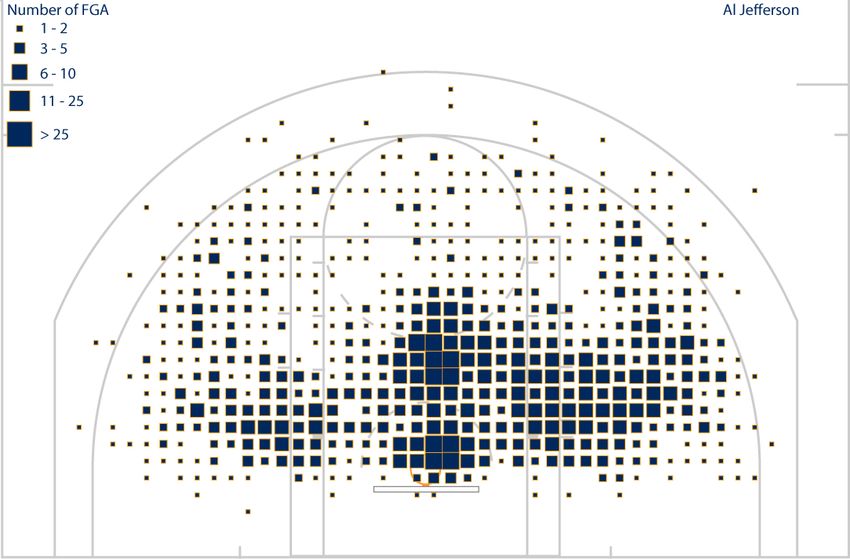
MIT Sloan Sports Analytics Conference 2012
                                              March 2-3, 2012, Boston, MA, USA

7 References
[1] T.C Bailey and A. C. Gatrell, Interactive Spatial Data Analysis, 1st Edition John
Wiley and Sons, New York, NY, 1995
[2] S. Fotheringham and C. Brunsdon, et al., Quantitative Geography: Perspectives
on Spatial Analysis. Sage Publications, London, UK, 2000.

[3] R. Haining, Spatial Data Analysis. Theory and Practice. Cambridge University
Press, 2003.

[4] D.A. Hickson, and L.A. Waller, et al., Spatial Analyses of Basketball Shot Charts:
An Application to Michael Jordan’s 2001-2002 NBA Season, Technical Report,
Department of Biostatistics, Emory University, 2003.

[5] B.J. Reich, J.S. Hodges, et al., A Spatial Analysis of Basketball Shot Chart Data,
The American Statistician, American Statistical Association, 60(1), pp 3-12, 2006.

[6] J. Piette, S. Anand, et al., Scoring and Shooting Abilities of NBA Players. Journal
of Quantitative Analysis in Sports, 6(1), 2010.

[7] J. Whelan, Why the Mavs’ zone defense will decide the Finals, hoopspeak.com.,
31 May 2011. Web. 12 Jan. 2012.

[8] J.J. Thomas and K.A. Cook, Illuminating the Path: The R&D Agenda for Visual
Analytics National Visualization and Analytics Center, 2005.

[9] Dean Oliver, Basketball on Paper: Rules and Tools for Performance Analysis,
Potomac Books Inc., 2004.

[10] John Hollinger, Pro Basketball Forecast: 2005-2006, Potomac Books Inc., 2005.

                                          7
You can also read