COVID-19 Frequency and accuracy of proactive testing for
←
→
Page content transcription
If your browser does not render page correctly, please read the page content below

Frequency and accuracy of proactive testing for
                 COVID-19
      Ted Bergstrom1 , Carl T. Bergstrom2 , and Haoran Li3
1
  University of California Santa Barbara, Economics Department
       2
         University of Washington, Department of Biology
3
  University of California Santa Barbara, Economics Department

                            September 6, 2020

                                   Abstract
        The SARS-CoV-2 coronavirus has proven difficult to control not only
    because of its high transmissibility, but because those who are infected
    readily spread the virus before symptoms appear, and because some in-
    fected individuals, though contagious, never exhibit symptoms. Proactive
    testing of asymptomatic individuals is therefore a powerful, and proba-
    bly necessary, tool for preventing widespread infection in many settings.
    This paper explores the effectiveness of alternative testing regimes, in
    which the frequency, the accuracy, and the delay between testing and re-
    sults determine the time path of infection. For a simple model of disease
    transmission, we present analytic formulas that determine the effect of
    testing on the expected number of days during which an infectious indi-
    vidual is exposed to the population at large. This allows us to estimate
    the frequency of testing that would be required to prevent uncontrolled
    outbreaks, and to explore the trade-offs between frequency, accuracy, and
    delay in achieving this objective. We conclude by discussing applications
    to outbreak control on college and university campuses.

    Competing Interest Statement: Ted Bergstrom and Haoran Li have
    no competing interests. Carl Bergstrom consults for Color Genomics on
    COVID testing schedules.

                                       1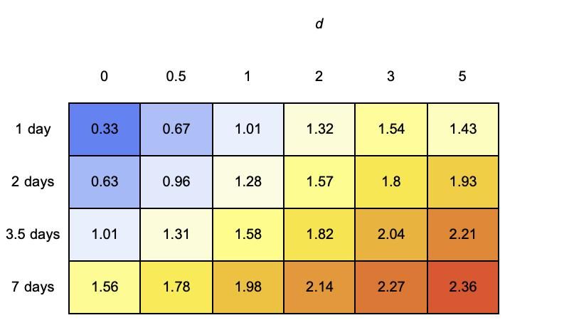
The SARS-CoV-2 coronavirus has infected six million people in the
United States as of late August 2020. Unlike the SARS virus which ap-
peared in 2003 [1, 2], SARS-CoV-2 is readily transmitted before symptoms
develop [3, 4, 5]. Entirely asymptomatic infections are common [6, 7, 8],
yet asymptomatic patients transmit disease. [9, 2, 10, 11]. The severity
of COVID varies from mild illness [12] to pneumonia and acute respira-
tory distress syndrome [13]. Symptoms are highly variable, and range
from respiratory to gastrointestinal, neurological to circulatory [14, 15].
As a consequence, neither symptomatic screening, nor self-isolation based
on symptoms is likely to identify the majority of cases [16, 17]. As a re-
sult, frequent proactive testing will be an important component of control,
because it can provide a surrogate for symptomology in identifying and
subsequently isolating infectious individuals [18].
    To the first order, the early dynamics of an epidemic are shaped by
a single parameter, the “basic reproduction number” R0 . This quantity
is defined as the expected number of secondary infections arising from an
index case in a wholly susceptible population [19]. In the initial stages
of an epidemic the number of cases can be expected grow exponentially
over time when R0 > 1. When R0 < 1, newly introduced infections will
result in only a limited number of cases. As an epidemic progresses and
the number of susceptible individuals declines, we look at the effective
reproductive number R = R0 S, where S is the fraction of the population
that remains susceptible to disease. To control the spread of disease, a
community, workplace, university, or other setting needs to ensure that R
remains below unity.
    The basic reproduction number is not an intrinsic property of the
virus, but rather reflects the organization and social behavior of a given
population at a particular time. Thus the basic reproduction number
varies across subpopulations, and changes in response to infection control
measures. A commonly used estimate of R0 for COVID, in the absence of
social distancing measures, is R0 = 2.5 [20]. Non-pharmaceutical interven-
tions such as face masks, social distancing, and limits on large gatherings
can reduce R0 somewhat, but are unlikely to drive the basic reproduction
number below unity without taking a dramatic toll on the social and eco-
nomic life of a community. Frequent proactive testing of asymptomatic
individuals offers an additional way to reduce transmission, and is among
the most powerful and least disruptive of non-pharmaceutical interven-
tions.
    How much testing is necessary to reduce R by a given amount? This
depends in intricate ways on the biology of the virus and the details of
the population in question—but a simple heuristic provides a nice ap-
proximation. Imagine that each infectious person is either at large in the
community or isolated at home during each day of the infectious period.
The number of contacts that an infectious person has will be roughly
proportional to the fraction of the infectious period spent at large. If
transmission is eliminated entirely while isolated, then to reduce R to 1,
it is necessary that reduce the average fraction of the infectious period
spent at large to 1/R. This means that if R = 2.5 in the absence of
testing, then to achieve R < 1 through testing and isolation, it would be
necessary to reduce the fraction of the time that infectious individuals are

                                     2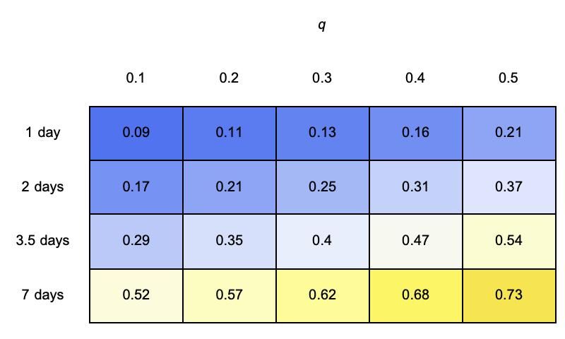
at large in the community by more than 60 percent.
    Communities face considerable variation and uncertainty regarding
COVID transmission rates, and in the effects that non-pharmaceutical
interventions have on transmission. There is also substantial variation
(and some uncertainty) in the sensitivities and specificities of alternative
testing methods, in the costs of these methods, and in the turnaround
times that these methods offer between testing and reporting. The inter-
actions between these effects is complex and non-linear. In this paper,
we develop analytic formulas that allow one to calculate the predicted
reduction in transmission rates that result, under alternative parameters
of infection from any specified testing regime.

Testing regime and contagious exposure
Testing plays multiple roles in pandemic control. Testing for individual
diagnosis is used to determine whether patients exhibiting disease symp-
toms are suffering from COVID or some other malady. Point-of-care test-
ing can serve to clear individuals to undergo medical or dental procedures,
or engage in other high-contact activity. Testing serves a surveillance role,
helping public health officials track the prevalence of disease and the rate
of spread. Finally, by proactively testing individuals who are not showing
symptoms, health workers can identify individuals who are infected but
do not realize it, and isolate them from interactions with the community.
We focus on this last role here.
    Throughout our discussion, we will assume that the course of coron-
avirus infection can be parameterized as follows:
Assumption 1 (Parameters of infection). A vector of infection parame-
ters γ = (C, u, v, y) is defined in the following way:
   • The infectious period for all cases, symptomatic or asymptomatic, is
     C days.
   • A fraction u of cases are asymptomatic
   • Among symptomatic cases, a fraction v self-isolate once the symp-
     toms appear and will no longer transmit disease.
   • Among symptomatic cases, there is a pre-symptomatic period y days
     during which a patient is infectious. This includes the time from the
     onset of the symptoms until the time that the patient realizes that
     isolation is warranted.
   Because symptoms vary and mild COVID symptoms can be confused
with seasonal allergies, a common cold, or other maladies, a majority of
symptomatic individuals may not quarantine. Larremore et al [21] as-
sume that only 20% of those who are infected self-isolate when symptoms
appear; Color Genomics [22] uses a slightly higher value of 30% for a
workplace population.
   Infected individuals who become symptomatic are contagious for an
average of approximately 3 days before symptoms appear [23]. There is

                                     3
substantial divergence in estimates of the average number of days of infec-
      tiousness after symptoms appear. The CDC1 cites studies that indicate
      that for those with mild symptoms, the number of days of infectious-
      ness after infection is “less than 10” according to one source and “less
      than 6” according to another source. Adding the number of days of pre-
      symptomatic contagion to the post-symptomatic number, it is reasonable
      to suppose that, on average, an infected person is infectious for 7 or 8
      days.
          Some infected individuals remain fully asymptomatic for the entire
      course of infection, and never develop any noticeable symptoms. The
      CDC estimates that approximately 40% of infected persons fit into this
      category [20].
          We have limited information about the sensitivity (defined as one mi-
      nus the false negative rate) of RNA-based tests for COVID, and much
      of what we do have is drawn from patients with serious illness. Esti-
      mating test sensitivities for pre-symptomatic and asymptomatic persons
      is especially difficult; we have found no studies that directly address the
      sensitivity for these populations. However, contact tracing studies [2], [10]
      indicate that asymptomatic and pre-symptomatic individuals carry sim-
      ilar viral loads to those with symptoms and thus are comparably likely
      to transmit disease. A survey of studies based on Chinese hospital pa-
      tients [24] reports test sensitivities ranging from 71% to 98%. A survey of
      research that includes some out-patient and in-patient cases by Kucirka
      et al. [25] estimates that the fraction of false-negatives ranges from 38%
      when symptoms first appear to 20% when symptoms disappear.2 In a
      brief article advising physicians on the interpretation of test results, Wat-
      son et al [26] observe that “As current studies show wide variation and
      are likely to overestimate sensitivity, we will use the lower end of current
      estimates from systematic reviews, with approximate sensitivity of 70%”
      (equivalently false-negative rate of 30%.)
          Given the considerable uncertainty around the test sensitivities and
      the variation across sample collection and testing methods, we treat this
      rate as a parameter which can be adjusted when calculating the effects of
      testing.
          We parameterize a testing regime as follows.
      Assumption 2 (Parameters of the testing regime). A testing regime
      τ = (n, q, d) is characterized as follows:
         • Everyone is tested at regular intervals, where n is the number of days
           between tests.
         • An infectious individual will have a false negative test result with
           probability q. (I.e., test sensitivity is 1 − q.) The probability that an
           infectious person has a false negative result on any test is indepen-
           dent of the results of prior tests taken while infectious.
         • After a delay of d days from the time of the test, those who test
           positive will be isolated for the remainder of their infectious period.
  1 https://www.cdc.gov/coronavirus/2019-ncov/hcp/duration-isolation.html
    2 Kucirca et al.   display a curve showing very high rates of false-negatives for pre-
symptomatics, but these estimates seem to be meaningless, since they result from a curve-
fitting exercise that uses only one pre-symptomatic observation.

                                            4
Definition 1 (Expected exposure function). The expected exposure func-
      tion E(C, τ ) is the expected amount of time that someone will be contagious
      and at large under testing regime τ if, in the absence of testing, they would
      be contagious and at large for a period of C.
          The expected exposure time depends on the parameters of infection
      and of the testing regime in a rather complex, non-linear way. In subse-
      quent discussion, we find explicit formulas for the expected exposure func-
      tion. We have developed a “Contagion Calculator” which can be found
      at https://steveli.shinyapps.io/FrequencyAndAccuracyCalculator/.
      With this calculator, one can input values for the parameters of infection
      and of the testing regime, and the the calculator will output expected
      exposure days for an infected person, the ratio of expected exposure days
      with testing to that with no testing, and an estimated effective reproduc-
      tive number R that would be achieved with this testing regime.

      Exposure ratios when testing intervals are longer
      than the period of infectiousness
      If testing intervals are longer than the period of infectiousness, then some
      infected persons will never be tested and those who are tested will be
      tested at most once while contagious. This makes calculation of exposure
      ratios relatively easy, but also means that testing will have only a small
      effect on the expected number of days that infected persons are exposed
      to the public while contagious. For example, at least one major university
      plans to test asymptomatic persons just once per month upon reopening3
      Our calculations show that with monthly testing, if all of those who test
      positive are isolated, will reduce their effective reproductive number R by
      less than 10 per cent.
          If the interval n between tests is longer than C − d, an infected person
      will be tested at most one time while contagious. Let the random variable
      t be the length of the period between the time when a subject first becomes
      infectious and the time of the next test. We assume that t is uniformly
      distributed on the interval [0, n] between tests.4 The results of a test for
      someone who has t= t > C −d will become available only after this person
      is no longer infectious. Thus this person will be contagiously exposed for
      the full period C of contagion. If t < C − d, then the subject will be
      infected when tested and will test positive and be isolated with probability
      1 − q. At the time of testing, the subject will have been contagiously
      exposed for a period of t before the test and will continue to be so for
      an additional time d until test results appear. Thus if the test reports
      accurately, the total time of contagious exposure will be t + d. It follows
      that the expected amount of time of contagious exposure for an infected
   3 According to the University of California at San Diego website,                   https://
returntolearn.ucsd.edu/return-to-campus/testing-and-screening/index.html (accessed
Sept 1, 2020), “The University is also planning to conduct periodic asymptomatic testing,
most likely on a monthly basis.”
   4 Even if testing occurs at fixed time intervals, the time at which infectiousness begins can

reasonably be viewed as distributed continuously

                                               5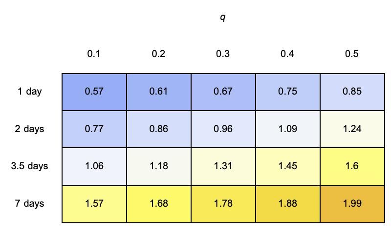
person is
                    Z   C−d                                 Z   n
                              1                                    1
       E(C, τ ) =               (1 − q)(t + d) + q C dt +             C dt    (1)
                    0
                              n                             C−d
                                                                    n

As we show in the Appendix, Equation 1 simplifies to yield the following
result:
Proposition 1. Given Assumption 2, if n > C − d,
                                         (1 − q)(C − d)2
                        E(C, τ ) = C −                                        (2)
                                                2n

Exposure ratios when testing intervals are shorter
than the period of infectiousness
When testing intervals are shorter than the period of infectiousness, every
infected person will be tested at least once during their infectious period.
Some, who are infected but test negative, may be tested again in time for
the results to be returned while they remain infectious. We assume that
the probability of a negative result for an infectious person on any test is
independent of the results of previous tests.
    We model the the amount of time between the onset of infectiousness
and the first time that a subject is tested as a random variable t drawn
from a uniform distribution on the interval [0, n]. Suppose that the time
interval from the beginning of infectiousness to a subject’s first test is
t < C − d. With probability 1 − q, the test will correctly report a positive
result. In this case, the subject will be isolated with a time delay of d
and will have been contagiously exposed to the public for a total duration
of t + d. With probability q, the first test incorrectly reports a negative
result. In this case, the subject test will be tested again after n days and
every n days thereafter so long as he or she continues to test negative. For
a subject who is first tested at an interval of t after becoming infectious,
let x(t) be the number of testing occasions that occur while this patient
remains infectious and would still be infectious when the test results come
back. This is the largest integer i such that t + d + n i ≤ C. Equivalently,
this is the largest integer i such that i ≤ (C − t − d)/n. We use a standard
notation b·c for the “floor” function to write the following definition:
                                                    C−d−t
Definition 2. Where 0 ≤ t ≤ C − d, let x(t) =          n
                                                                . Let x̄ = x(0) =
 C−d
   n
        , and let r = C − d − n x̄.
     When 0 ≤ i ≤ x(t), the probability that someone whose first test
occurs after being contagious for length of time t, who has i consecutive
false negative results, and who tests positive on the next occasion, is
(1 − q)q i . In this event, the number of days of infectious exposure would
be t+n i+d ≤ C. With probability q x(t)+1 , an infectious person will never
be isolated while contagious, and thus will be infectious and at large for
C days.
     It follows that where the contagious period is C days and the testing
regime is τ = (n, q, d), the expected number of days of contagious exposure
for someone who is first tested after being contagious for a length of time
t is

                                         6
x(t)
X
Et (C, τ ) = (1 − q) (t + n i + d)q i + C q x(t)+1 . (3)
i=0
Since t is assumed to be uniformly distributed on the interval [0, n],
the expected number of days of contagious exposure for an infected person
is Z n
1
E(C, τ ) = Et (C, τ )dt. (4)
0
n
In the Appendix we show that Equations 3 and 4 imply the following
proposition:
Proposition 2. Given Assumptions 1 and 2, if n ≤ C − d,
n nq 1 nq
+ q x̄ qr2 − (n − r)2 −
E(C, τ ) = +d+ (5)
2 1−q 2n 1−q
where x̄ and r are defined in Definition 2.
We will use the formula that appears in Proposition 2 to calculate the
exposure ratio and the estimated R values under some alternative testing
regimes, under plausible assumptions about the parameters of infection.
Self-isolation for some with symptoms
Even without testing, some individuals will choose to self-isolate once
symptoms become evident. The number of days of contagious exposure
for these individuals will include only those days when they are contagious
before symptoms appear. With infection parameters γ = (C, u, v, y), the
fraction (1 − u) of infected individuals will display some symptoms. Of
these, the fraction v will self-isolate when symptoms appear. Thus the
fraction of infected persons who self-isolate is v(1 − u) and the fraction
who do not do so is 1 − v(1 − u). If infected individuals are contagious
for a time period of y days before symptoms appear, then the expected
amount of contagious exposure time for these individuals is E(y, τ ).
It will be convenient to define the following functions that relate the
parameters of infection and the testing regime to contagious exposure
when some symptomatic individuals self-isolate.
Definition 3 (Exposure functions). Where γ = (C, u, v, y) and τ =
(n, q, d) denote the parameters of exposure and of the testing regime, let
Ent (γ) be the expected number of days of contagious exposure for an in-
fected person with no testing, and let Ē(γ, τ ) be the expected number of
days of contagious exposure with testing regime τ .
The expected number of exposure days for an infected individual is a
weighted average of the number of exposure days for those who self-isolate
and those who don’t. The fraction of infected individuals who self-isolate
is (1 − u)v and the fraction who do not self-isolate is 1 − (1 − u)v. With
infection parameters γ and testing regime τ , the expected number of days
of exposure for an infected person who self-isolates will be E(y, τ ) and
for one who does not self-isolate will be E(C, τ ). The expected number
7of days of contagious exposure for a randomly selected infected person is
then:
Ē(γ, τ ) = 1 − (1 − u)v E(C, τ ) + (1 − u)v E(y, τ ). (6)
With infection parameters γ = (C, u, v, y), and with no testing, the ex-
pected number of days of exposure for an infected person will be
Ent (γ) = 1 − (1 − u)v C + (1 − u)v y
= C − (1 − u)v(C − y) (7)
Definition 4 (Exposure ratio function). We define
Ē(γ, τ )
ExpRat(γ, τ ) =
Ent (γ)
to be the ratio of the expected amount of time that a contagious person is
exposed to the public with testing regime τ to that if there is no testing.
For any value of the reproduction number Rnt that would apply with-
out testing, we can use the expected exposure ratio to estimate the value
of R that would apply given testing regime τ .
Definition 5 (Estimated R-with-testing). The function R̃ (γ, τ, Rnt ) is
the estimated basic reproduction number R that results from testing regime
τ , the vector of infection parameters is γ and where the R value without
testing is Rnt .
Assuming that the expected number of people that one infects is pro-
portional to the amount of time one is exposed to the population while
contagious, we have the following simple relationship.
R̃(γ, τ, Rnt ) = ExpRat (γ, τ ) Rnt (8)
Estimated exposure ratios and R values
with testing
We used the contagion calculator found at https://steveli.shinyapps.io/
FrequencyAndAccuracyCalculator/ to explore the estimated exposure ra-
tios and R values under alternative assumptions about the frequency, ac-
curacy, and delay from test to isolation of testing regimes, given plausible
infection parameters.
Tables 1-4 show estimated exposure ratios under various testing regimes.
Throughout, we have assumed that in the absence of testing an infected
person is contagious for C = 8 days, that those who display symptoms
will do so after y = 3 days, that a fraction u = 0.4 of infected persons
are asymptomatic, that R = 2.5, and that v = 0.3 of those who have
symptoms will self-isolate without testing, four days after becoming con-
tagious.
8Table 1: Exposure ratio with delay d = 1
Table 2: Estimated R if d = 1 and R is 2.5 without testing
Trade-offs between frequency and accuracy
Tables 1 and 2 illustrate the effects of test sensitivity on the exposure
ratios and estimated effective reproductive number R, for various testing
rates.
These tables indicate that if R = 2.5 in the absence of testing, a daily
test with a one day delay could reduce R below unity even with a false
negative rate of fifty percent. With a false negative rate of thirty percent,
testing every second day would result in R < 1. With a false negative
rate of ten percent, testing twice per week would get R very close to
unity. Testing once per week would not bring R values close to 1.
9Trade-offs between delay and frequency
Tables 3 and 4 illustrate the effects of the delay between testing and
isolation. These tables display the exposure ratio and estimated R for the
stated test frequencies and delays, assuming a false negative rate of thirty
percent.
Table 3: Exposure ratio, report delay, and test frequency
Table 4: Estimated R, report delay, and test frequency
The effect of reducing the delay between testing and isolation from
two days to one day is similar to that of increasing test frequency from
every second day to every day, or from twice a week to every second day.
If the delay can be shortened from one day to half a day, exposure rates
are further reduced by about twenty percent. The tables show that with
a five-day delay, testing becomes almost worthless for reducing exposure
and with a three day delay, even everyday testing falls short of reducing
contagious exposure by fifty percent.
10Point-of-care testing
The US Food and Drug Administration has recently posted a template
for commercial developers to help them develop simple COVID tests for
which results could be determined on-site within minutes. In releasing
this template, FDA Commissioner Stephen M. Hahn, M.D. said that5
“We hope that with the innovation we’ve seen in test de-
velopment, we could see tests that you could buy at a drug
store, swab your nose or collect saliva, run the test, and re-
ceive results within minutes at home, once these tests become
available.”
If such a test becomes available relatively cheaply, it would then be
feasible to test very frequently with no significant delay between testing
and isolation. Even if such a test had a relatively high probability of
false negatives (low sensitivity), the ability to test frequently with quick
response would permit frequent testing to drastically reduce the exposure
ratio. Tables 5 and 6 show the exposure ratios and estimated R values as
a function of test accuracy and frequency when test results are available
immediately.
Table 5: Exposure ratio when test results are immediate
Table 5 shows that a test with very low sensitivity, if it can be ad-
ministered every day with results appearing immediately, can drastically
reduce the exposure rate. Indeed if those who test positive are quaran-
tined immediately on taking a test administered daily, with sensitivity of
50%, the number of days of contagious exposure for infected persons is
reduced by almost 80%. This compares with a reduction of about 60%
that results from testing twice a week with a test with sensitivity of 90%.
5 Quoted on July 29, 2020 at https://www.fda.gov/news-events/press-announcements/
coronavirus-covid-19-update-fda-posts-new-template-home-and-over-counter-
diagnostic-tests-use-non
11Table 6: Estimated R when test results are immediate
Discussion
As an increasing diversity of testing technologies receive emergency use
authorization, communities are able to consider a broader range of possible
testing strategies to contribute to COVID control. Any testing approach
comes with tradeoffs: various tests differ in cost, convenience, sensitivity,
inconclusive rate, and processing time.For example, saliva samples are
easier to collect and less onerous to donate to collect than samples taken
by nasopharyngeal swabs. Even if there were some reduction in sensitiv-
ity, these advantages could allow for more frequent collection and make
saliva samples the preferred method. The use of pooled samples could
substantially reduce the cost of testing, but might increase the fraction
of false negative readings and possibly increase the delay between testing
and reported results.6
To manage COVID within a community, it will be critical to assess
how these tradeoffs play into optimal choice of testing strategies. While
simulations can be useful in this endeavor, the sheer number of possible
approaches will quickly overwhelm the ability to exhaustively explore all
options using computationally intensive methods. The model and calcu-
lator we have presented here provide an alternative. Our analytic ap-
proximations can be used explore trade-offs between such variables as
the frequency of testing, the sensitivity of testing, and the delay between
testing and results.
Proactive testing is likely to be particularly important in college and
university settings. Because students live in close proximity and engage in
frequent interpersonal interactions, we would expect R0 on campuses to
be high compared to nationwide averages. In addition, young adults ap-
6 In one basic approach to pooled sampling, half of the material from each subject is used in
the pooled sample and half is withheld to be tested in case the pooled sample result is positive.
If there is a positive result with the pooled sample, then the remainder of the material collected
from each subject is tested. This retesting might add a half day or more to the time before
the result are returned.
12pear more likely to experience subclinical disease [27] and thus less likely
to self-isolate based on symptoms. Large clusters have already occurred
in these university settings during summer sessions [28] and at schools
attempting an in-person autumn semester [29]. In the absence of aggres-
sive mitigation, colleges are likely to function as tinderboxes from which
devastating epidemics emerge. Even if college-aged students are at lower
risk for disease, on-campus clusters spread disease into more vulnerable
populations in the surrounding communities [30].
Our results, and the results of other models[18, 31, 32], indicate that by
proactively screening asymptomatic individuals and isolating those who
test positive, universities should be able to substantially reduce the rate
at which COVID spreads on campus. Yet the Centers for Disease Con-
trol chose to explicitly not recommend entry testing or ongoing testing of
asymptomatic individuals on college campuses [28]. Taking this as absolu-
tion, many university administrators have failed to consider the possibility
of frequently testing the entire student body and staff, on the grounds that
doing is unnecessary, infeasible, and excessively costly7 . A recent study
examined the fall reopening plans of more than 500 universities as of Au-
gust 7, 2020 [34]. The study reports that only about 27% of them plan to
do some form of re-entry testing as students first arrive on campus and
only about 20% plan to do some regular testing of all students.
Many of the exceptions are smaller East Coast institutions, a number
of which are testing their students twice weekly in collaboration with the
help of the Broad Institute [34]. The University of Illinois (UIUC) stands
out among large public institutions in having implemented an in-house
testing program that will administer saliva-based COVID-19 tests twice
a week to each of its roughly 50,000 students and faculty.8 These tests,
which have been developed in the university’s own laboratories have been
found to be about as accurate as conventional PCR-based testing, and
they offer approximately 5 hour turnaround between test administration
and reported results.
Although many universities lack the resources and planning capability
to apply regular testing and quarantine for their fall terms, cheaper and
quicker tests appear to be on the horizon, and seem to be largely deterred
by the lack of FDA approval [35]. Simple self-administered, paper-strip
antigen tests have been developed by the Wyss Institute at Harvard and
can be made available at a cost of $1-$5 per test. [35, 36]. As explained
by Kotlikoff and Mina [35],
You would simply spit into a tube of saline solution and
insert a small piece of paper embedded with a strip of protein.
If you are infected with enough of the virus, the strip will
change color within 15 minutes.
7 The president of the University of Michigan, Dr. Mark Schlissel maintains that for a
large university such as Michigan, regular testing of students and staff is simply impossible.
According to Dr. Schlissel, “This notion that a university at the scale of Michigan can test
everybody a couple of times a week or every day, right now, that’s science fiction.” [33]
8 Current statistics on tests administered and the number of positive results are found at
the UIUC dashboard https://splunk-public.machinedata.illinois.edu:8000/en-US/app/
uofi shield public APP/home.
13These tests may not be as sensitive as standard RNA-based tests, but
their cost and ease of testing would make it possible for them to be used
by all community members every day, with results available immediately.
Thus they are almost certain to be more effective in reducing the spread
of the epidemic than more sensitive tests administered less frequently and
with slower turnaround.
The model that we have developed here is analytically tractable be-
cause we have made certain simplifying assumptions about the nature of
disease transmission. Perhaps foremost among these simplifications is the
assumption that transmission rates are a step function: individuals who
have COVID go from non-infectious to fully infectious instantaneously,
and remain fully infectious until they are no longer able to transmit dis-
ease. Test sensitivity takes the same form over the course of infection.
More sophisticated models could allow varying infectiousness and varying
sensitivity over time, as in ref. [18]. In the absence of compelling data
about the actual time-course of infectiousness and detectability, we have
opted for the simple form analyzed here.
In our analysis we assume homogeneous susceptibility, transmissibility,
and timing of the disease course across all individuals. Heterogeneity in
disease parameters can have sizeable impacts on disease dynamics, but
this is less of an problem than it might seem for what we are doing here.
Our aim is not to explicitly model the dynamics of an outbreak, but rather
to estimate the change in the frequency of transmission events. By doing
so, we can compare the relative efficacy of alternative testing strategies
and identify conditions under which testing will be sufficient to drop the
effective reproductive number below unity. For this purpose, it is largely
sufficient to work with mean parameter values. The major advantage
to the approach we take here is that the analytic approximations enable
more complex comparative static analysis and optimization efforts than
would be feasible using time-consuming simulations. We hope that our
findings will prove useful in this way to those involved in selecting testing
procedures for colleges, workplaces, communities, and other groups.
14Appendix
Proof of Proposition 1
Proof.
Z C−d Z n
1 1
E(C, n) = ((1 − q)(t + d) + qC)dt + Cdt
0
n C−d
n
(1 − q)(C − d)2 (1 − q)(C − d)d q(C − d) n − (C − d)
= + + C+ C
2n
n n n
C − d (1 − q)(C − d)
= + (1 − q)d + qC − C + C
n 2
C −d (1 − q)(C − d)
= + (1 − q)d − (1 − q)C +C
n 2
(1 − q)(C − d) (C − d)
= +d−C +C
n 2
(1 − q)(C − d) d − C
= +C
n 2
(1 − q)(C − d)(d − C)
= +C
2n
(1 − q)(C − d)2
= C− (9)
2n
Proof of Proposition 2
The following lemma will be useful for simplifying Equation 3.
Lemma 1. Where 0 ≤ q < 1,
x
X i−1 1 1
(1 − q) iq = − qx +x .
1−q 1−q
i=1
Proof of Lemma 1.
x x
X X d
(1 − q) iq i−1 = (1 − q) qi
dq
i=1 i=1
x
d X i
= (1 − q) q
dq
i=1
d 1 − q x+1
= (1 − q) −1
dq 1−q
1 − (x + 1)q x + xq x+1
= (1 − q)
(1 − q)2
1 1 + x(1 − q)
= − qx
1−q 1−q
1 1
= − qx +x
1−q 1−q
15Proof of Proposition 2. From Equation 3 and Lemma 1, it follows that
x(t) x(t)
X X
Et (C, n) = (1 − q) (t + d)q i + (1 − q)nq iq i−1 + Cq x(t)+1
i=0 i=1
x(t)+1 nq 1
− nq x(t)+1 + Cq x(t)+1
= (t + d) 1 − q + + x(t)
1−q 1−q
nq q
(t + d) 1 − q x(t)+1 + − nq x(t)+1 + Cq x(t)+1
= + 1 + x(t)
1−q 1−q
nq q
= t+d+ + q x(t)+1 C −d−n + x(t) + 1 −t (10)
1−q 1−q
Since t is assumed to be uniformly distributed on the interval [0, n],
the expected number of days of contagious exposure for an infected person
is Z n
1
E(C, n) = Et (C, n)dt (11)
0
n
Equation 11 is more manageable than it first appears, because the
function x(t) takes on only two values over its range. This is explained
by the following lemmas.
A−b
Lemma 2. For any A > n, if A n
= x and r = A − nx, then n
=x
if 0 ≤ b ≤ r and A−b
n
= x − 1 if r < b ≤ r + n.
Where r = (C − d) − n C−d , and x ≤ r, it follows from Lemma 2
n
that if x ≤ r, then x(t) = C−d
n
if t ≤ r, and x(t) = C−dn
− 1. if t > r,
Thus we have
Lemma 3. Let x̄ = x(0) = C−dn
. Where x(t) = C−t−d n
and r =
C−d
C − d − n n , we have x(t) = x̄ if t ≤ r and x(t) = x̄ − 1 if t > r.
C−d
Where r = C − d − n n
, and x̄ = x(0), we have
Z r Z n
1 1
E(C, n) = Et (C, n)dt + Et (C, n)dt. (12)
n 0
n r
Then
r r r
q x̄+1
Z Z Z
1 1 nq q
Et (C, n)dt = t+d+ dt + C −d−n + x̄ + 1 − t dt
n 0
n 0
1−q n 0
1−q
r2 r nq r q r2
= + d+ + q x̄+1 (C − d − nx̄) − n +1 − q x̄+1
2n n 1−q n 1−q 2n
r2 r nq x̄+1 r nq r2
= + d+ +q r− −n − q x̄+1
2n n 1−q n 1−q 2n
r2 r nq x̄+1 r n r2
= + d+ +q r− − q x̄+1
2n n 1−q n 1−q 2n
r2 r nq r2 r nq
= + d+ + q x̄+1 − q x̄ (13)
2n n 1−q 2n n 1−q
16and
Z n Z n
1 1 nq x̄ q
Et (C, n)dt = t+d+ +q C −d−n + x̄ −t dt
n r
n r
1−q 1−q
n2 − r2 n−r nq x̄ n −r nq x̄ n2 r2
= + d+ +q r− −q −
2n n 1−q n 1−q 2n 2n
n2 − r2 n−r nq x̄ n −r nq n+r
= + d+ +q r− −
2n n 1−q n 1−q 2
n2 − r2 n−r nq n−r r n n − r x̄ nq
= + d+ + q x̄ − − q (14)
2n n 1−q n 2 2 n 1−q
Equations 12, 13, and 14 imply that
n nq r2 (n − r)2 nq
E(C, n) = +d+ + q x+1 − q x̄ − q x̄
2 1−q 2n 2n 1−q
n nq x̄ 1 nq
qr2 − (n − r)2 −
= +d+ +q (15)
2 1−q 2n 1−q
References
[1] David M Bell et al. Public health interventions and sars spread, 2003.
Emerging Infectious Diseases, 10(11):1900, 2004.
[2] Monica Gandhi, Deborah S Yokoe, and Diane V Havlir. Asymp-
tomatic transmission, the achilles’ heel of current strategies to control
covid-19. New England Journal of Medicine, 2020.
[3] Anne Kimball, Kelly M Hatfield, Melissa Arons, Allison James,
Joanne Taylor, Kevin Spicer, Ana C Bardossy, Lisa P Oakley,
Sukarma Tanwar, Zeshan Chisty, et al. Asymptomatic and presymp-
tomatic sars-cov-2 infections in residents of a long-term care skilled
nursing facility—king county, washington, march 2020. Morbidity
and Mortality Weekly Report, 69(13):377, 2020.
[4] Xi He, Eric HY Lau, Peng Wu, Xilong Deng, Jian Wang, Xinxin
Hao, Yiu Chung Lau, Jessica Y Wong, Yujuan Guan, Xinghua Tan,
et al. Temporal dynamics in viral shedding and transmissibility of
covid-19. Nature medicine, 26(5):672–675, 2020.
[5] Lauren Tindale, Michelle Coombe, Jessica E Stockdale, Emma Gar-
lock, Wing Yin Venus Lau, Manu Saraswat, Yen-Hsiang Brian Lee,
Louxin Zhang, Dongxuan Chen, Jacco Wallinga, et al. Transmis-
sion interval estimates suggest pre-symptomatic spread of covid-19.
MedRxiv, 2020.
[6] Hiroshi Nishiura, Tetsuro Kobayashi, Takeshi Miyama, Ayako
Suzuki, Sung-mok Jung, Katsuma Hayashi, Ryo Kinoshita, Yichi
Yang, Baoyin Yuan, Andrei R Akhmetzhanov, et al. Estimation of
the asymptomatic ratio of novel coronavirus infections (covid-19).
International journal of infectious diseases, 94:154, 2020.
17[7] Thomas A Treibel, Charlotte Manisty, Maudrian Burton, Áine McK-
night, Jonathan Lambourne, João B Augusto, Xosé Couto-Parada,
Teresa Cutino-Moguel, Mahdad Noursadeghi, and James C Moon.
Covid-19: Pcr screening of asymptomatic health-care workers at lon-
don hospital. The Lancet, 395(10237):1608–1610, 2020.
[8] Daniel P Oran and Eric J Topol. Prevalence of asymptomatic sars-
cov-2 infection: A narrative review. Annals of Internal Medicine,
2020.
[9] Yan Bai, Lingsheng Yao, Tao Wei, Fei Tian, Dong-Yan Jin, Lijuan
Chen, and Meiyun Wang. Presumed asymptomatic carrier transmis-
sion of covid-19. Jama, 323(14):1406–1407, 2020.
[10] Salynn Boyles. Covid-19: Asymptomatic transmission fueled nursing
home death toll. Physicians’ Weekly, April 2020.
[11] Jon C Emery, Timothy W Russell, Yang Liu, Joel Hellewell, Carl AB
Pearson, Gwenan M Knight, Rosalind M Eggo, Adam J Kucharski,
Sebastian Funk, Stefan Flasche, et al. The contribution of asymp-
tomatic sars-cov-2 infections to transmission on the diamond princess
cruise ship. eLife, 9:e58699, 2020.
[12] Rajesh T Gandhi, John B Lynch, and Carlos del Rio. Mild or mod-
erate covid-19. New England Journal of Medicine, 2020.
[13] John J Marini and Luciano Gattinoni. Management of covid-19 res-
piratory distress. Jama, 2020.
[14] Rachel M Burke. Symptom profiles of a convenience sample of pa-
tients with covid-19—united states, january–april 2020. MMWR.
Morbidity and Mortality Weekly Report, 69, 2020.
[15] Leiwen Fu, Bingyi Wang, Tanwei Yuan, Xiaoting Chen, Yunlong Ao,
Tom Fitzpatrick, Peiyang Li, Yiguo Zhou, Yifan Lin, Qibin Duan,
et al. Clinical characteristics of coronavirus disease 2019 (covid-19) in
china: a systematic review and meta-analysis. Journal of Infection,
2020.
[16] Katelyn Gostic, Ana CR Gomez, Riley O Mummah, Adam J
Kucharski, and James O Lloyd-Smith. Estimated effectiveness of
symptom and risk screening to prevent the spread of covid-19. Elife,
9:e55570, 2020.
[17] Seyed M Moghadas, Meagan C Fitzpatrick, Pratha Sah, Abhishek
Pandey, Affan Shoukat, Burton H Singer, and Alison P Galvani.
The implications of silent transmission for the control of covid-19
outbreaks. Proceedings of the National Academy of Sciences, 2020.
[18] Daniel B Larremore, Bryan Wilder, Evan Lester, Soraya Shehata,
James M Burke, James A Hay, Milind Tambe, Michael J Mina,
and Roy Parker. Test sensitivity is secondary to frequency and
turnaround time for covid-19 surveillance. medRxiv, 2020.
[19] Klaus Dietz. The estimation of the basic reproduction number for
infectious diseases. Statistical methods in medical research, 2(1):23–
41, 1993.
18[20] Covid-19 pandemic planning scenarios, 10 july 2020. Technical re-
port, Centers for Disease Control, 2020.
[21] Daniel Larremore et al. Test sensitivity is secondary to frequency and
turnaround time for covid-19 surveillance. MedRxiv, 2020. Preprint
posted June 27,2020, https://www.medrxiv.org/content/10.1101/
2020.06.22.20136309v2.
[22] Color Genomics. Impact of proactive testing. August 2020. web
simulation.
[23] Miriam Casey et al. Pre-symptomatic transmission of sars-cov-2 in-
fection: a secondary analysis using published data. MedRxiv, 2020.
Preprint posted June 11, 2020, https://www.medrxiv.org/content/
10.1101/2020.05.08.20094870v2.
[24] Ingrid Arevalo-Rodriquez et al. False-negative results of initial rt-pcr
assays for covid-19” a systematic review. MedRxiv, 2020.
[25] Lauren Kucirka et al. Variation in false-negative rate of reverse tran-
scriptase polymerase chain reaction–based sars-cov-2 tests by time
since exposure. Annals of Internal Medicine, May 2020.
[26] Jessica Watson, Penny F. Whiting, and John E. Brush. Interpreting
a covid-19 test result. British Medical Journal, May 2020.
[27] G Davies Nicholas, Klepac Petra, Liu Yang, Prem Kiesha, Jit
Mark, M Rosalind, CMMID COVID-19 working group, et al. Age-
dependent effects in the transmission and control of covid-19 epi-
demics. Nature Medicine, 2020.
[28] Carl T. Bergstrom. The cdc is wrong. Chronicle of Higher Education,
2020.
[29] New York Times Staff. Tracking coronavirus cases at u.s. colleges
and universities. New York Times, August 26 2020.
[30] Daniel Mangrum and Paul Niekamp. College student contribution to
local covid-19 spread: Evidence from university spring break timing.
Available at SSRN 3606811, 2020.
[31] Lee Kennedy-Shaffer, Michael Baym, and William Hanage. Perfect
as the enemy of the good: Using low-sensitivity tests to mitigate
sars-cov-2 outbreaks. 2020.
[32] Joshua S Gans. Test sensitivity for infection versus infectiousness of
sars-cov-2. Available at SSRN 3682242, 2020.
[33] Ann Zaniewski. Schlissel to faculty: Despite covid-19 u-
m’s commitment has not wavered. University of Michi-
gan: The University Record, August 13 2020. online at
https://record.umich.edu/articles/schlissel-to-faculty-
despite-pandemic-u-ms-commitment-has-not-wavered/.
[34] A Sina Booeshaghi, Fayth Hui Tan, Benjamin Renton, Zackary
Berger, and Lior Pachter. Markedly heterogeneous COVID-
19 testing plans among us colleges and universities. MedRxiv,
2020. Preprint posted August 11, 2020, https://www.medrxiv.org/
content/10.1101/2020.08.09.20171223v1.full.pdf+html.
19[35] Laurence Kotlikoff and Michael Mina. A cheap simple way to control
the coronovirus. New York Times, Opinion Article, July 3 2020.
[36] Alvin Powell. Cheap daily COVID tests could be ‘akin to vac-
cine’, professor says. Harvard Gazette, August 11 2020. On-
line at https://news.harvard.edu/gazette/story/2020/08/cheap-
daily-covid-tests-could-be-akin-to-vaccine/.
20You can also read