ShyLU: A Hybrid-Hybrid Solver for Multicore Platforms
←
→
Page content transcription
If your browser does not render page correctly, please read the page content below
ShyLU: A Hybrid-Hybrid Solver for Multicore Platforms

                    Sivasankaran Rajamanickam1 , Erik G. Boman1 , and Michael A. Heroux1 ,
                           E-mail:{srajama@sandia.gov, egboman@sandia.gov and maherou@sandia.gov}
                                              1   Sandia National Laboratories.

   Abstract—With the ubiquity of multicore processors, it is      in parallel on the compute node. Our hybrid-hybrid method
crucial that solvers adapt to the hierarchical structure of       is “hybrid” in two ways: the solver combines direct and
modern architectures. We present ShyLU, a “hybrid-hybrid”         iterative algorithms, and uses MPI and threads in a hybrid
solver for general sparse linear systems that is hybrid in two
ways: First, it combines direct and iterative methods. The        programming approach.
iterative part is based on approximate Schur complements             In order to be scalable and robust it is important for
where we compute the approximate Schur complement using           solvers and preconditioners to use the hybrid approach in
a value-based dropping strategy or structure-based probing        both meanings of the word. The hybrid programming model
strategy.                                                         ensures good scalability within the node and the hybrid
   Second, the solver uses two levels of parallelism via hybrid
programming (MPI+threads). ShyLU is useful both in shared-        algorithm ensures robustness of the solver. A sparse direct
memory environments and on large parallel computers with          solver is very robust and the BLAS based implementations
distributed memory. In the latter case, it should be used as a    are capable of performing near the peak performance of
subdomain solver. We argue that with the increasing complexity    desktop systems for specific problems. However, they have
of compute nodes, it is important to exploit multiple levels of   high memory requirements and poor scalability in distributed
parallelism even within a single compute node.
   We show the robustness of ShyLU against other algebraic
                                                                  memory systems. An iterative solver, while highly scalable
preconditioners. ShyLU scales well up to 384 cores for a          and customizable for problem specific parameters, is not
given problem size. We also study the MPI-only performance        as robust as a direct solver. A hybrid preconditioner can
of ShyLU against a hybrid implementation and conclude             be conceptually viewed as a middle ground between an
that on present multicore nodes MPI-only implementation is        incomplete factorization and a direct solver.
better. However, for future multicore machines (96 or more
cores) hybrid/ hierarchical algorithms and implementations are    A. ShyLU Scope and Our Contributions
important for sustained performance.
                                                                     Current iterative solvers and preconditioners (such as
                                                                  ML [1] or Hypre [2]) need a node level strategy in order
                     I. I NTRODUCTION
                                                                  to scale well in large petascale systems where the degree of
   The general trend in computer architectures is towards         parallelism is extremely high. The natural way to overcome
hierarchical designs with increasing node level parallelism.      this limitation is to introduce a new level of parallelism in the
In order to scale well in these architectures, applications       solver. We envision three levels of parallelism: At the top,
need hybrid/hierarchical algorithms for the performance           there is the inter-node parallelism (typically implemented
critical components. The solution of sparse linear systems        with MPI) and two levels of parallelism (MPI+threads) on
is an important kernel in scientific computing. A diverse         the node. Section V describes the various options to use
set of algorithms is used to solve linear systems, from           a parallel node level preconditioner with three levels of
direct solvers to iterative solvers. A common strategy for        parallelism.
solving large linear systems on large parallel computers,            The node level is where the degree of parallelism is
is to first employ domain decomposition (e.g., additive           rapidly increasing and this is the scope of ShyLU. Previous
Schwarz) on the matrix to break it into subproblems that          Schur/hybrid solvers all solve the global problem, competing
can then be solved in parallel on each core or on each            with multigrid. This approach instead complements the
compute node. Typically, applications run one MPI process         multigrid methods and focuses on the scalability on the node.
per core, and one subdomain per MPI process. A drawback           In this paper, we concentrate on the node level parallelism
of domain decomposition solvers or preconditioners is that        and leave the integration into the third (inter-node) level as
the number of iterations to solve the linear system will          future work.
increase with the number of subdomains. With the rapid               Our first contribution is a new scalable hybrid sparse
increase in the number of cores one subdomain per core is         solver, ShyLU (Scalable Hybrid LU, pronounced Shy-Loo),
no longer a viable approach. However, one subdomain per           based on the Schur complement framework. ShyLU is based
node is reasonable since the recent and future increases in       on Trilinos [3] and also intended to become a Trilinos
parallelism are and will be primarily on the node. Thus, an       package. It is designed to be a “black box” algebraic solver
increasingly important problem is to solve linear systems         that can be used on a wide range of problems. Furthermore,
it is suitable both as a solver on a single-node multicore
workstation and as a subdomain solver on a compute node
of a petaflop system. Our target is computers with many
CPU-like cores, not GPUs.
   Second, we revisit every step of the Schur complement
framework to exploit node level parallelism and to improve
the robustness of ShyLU as a preconditioner. ShyLU uses a
new probing technique that exploits recent improvements in
parallel coloring algorithms to get a better approximation of
the Schur complement.
   Third, we try to answer the question: “When will the            Figure 1. Partitioning and reordering of a (a) nonsymmetric matrix and
                                                                   (b) symmetric matrix.
hybrid implementation of a complex algorithm be better
than a pure MPI-based implementation?”. We use ShyLU as
our target “application” as a complex algorithm like linear        in both the mathematical and in the parallel programming
solver, with a pure MPI-based implementation and a hybrid          sense. In contrast to the other hybrid solvers our target is a
MPI+Threads implementation should be able to provide a             multicore node. See section IV for how these solvers differ
reasonable answer to this question. The answer is dependent        from ShyLU in the different steps of the Schur complement
on algorithms, future changes in architectures, problem sizes      framework.
and various other factors. We address this question for our
specific algorithm and our target applications.                              II. S CHUR C OMPLEMENT F RAMEWORK
                                                                     This section describes the framework to solve linear
B. Previous work
                                                                   systems based on the Schur complement approach. There
   Many good parallel solver libraries have been developed         has been lot of work done in this area; see for example,
over the last decades; for example, PETSc [4], Hypre [2],          Saad [17, Ch.14] and the references therein.
and Trilinos [3]. These were mainly designed for solving
large distributed systems over many processors. ShyLU’s            A. Schur complement formulation
focus is on solving medium-sized systems on a single com-             Let Ax = b be the system of interest. Suppose A has the
pute node. This may be a subproblem within a larger parallel       form
context. Some parallel sparse direct solvers (e.g., SuperLU-
                                                                                               D C

MT [5], [6] or Pardiso [7]) have shown good performance                                 A=              ,                 (1)
                                                                                               R G
in shared-memory environments, while distributed-memory
solvers (for example MUMPS [8], [9]) have limited scalabil-        where D and G are square and D is non-singular. The Schur
ity. Pastix [10] is an interesting sparse direct solver because    complement after elimination of the top row is S = G − R ∗
it uses hybrid parallel programming with both MPI and              D−1 C. Solving Ax = b then consists of solving
threads. However, any direct solver will require lots of mem-

                                                                                   D C           x1        b
ory due to fill-in and they are not ready to handle the O(100)                              ×         = 1                 (2)
                                                                                    R G          x2        b2
to O(1000) expected increase in the node concurrency (in
their present form at least). To reduce memory requirements,       by solving
incomplete factorizations is a natural choice. There are only         1) Dz = b1 .
few parallel codes available for incomplete factorizations in         2) Sx2 = b2 − Rz.
modern architectures. (e.g., [11], [12])                              3) Dx1 = b1 − Cx2 .
   Recently, there has been much interest in hybrid solvers           The algorithms that use this formulation to solve the
that combine features of both direct and iterative meth-           linear system in an iterative method or a hybrid method
ods. Typically, they partially factor a matrix using direct        essentially use three basic steps. We like to call this the
methods and use iterative methods on the remaining Schur           Schur complement framework:
complement. Parallel codes of this type include HIPS [13],            Partitioning: The key idea is to permute A to get a D that
MaPhys [14], and PDSLin [15]. ShyLU is similar to these            is easy to factor. Typically, D is diagonal, banded or block
solvers in a conceptual way that all these solvers fall into the   diagonal and can be solved quickly using direct methods.
broad Schur complement framework described in section II.          As the focus is on parallel computing, we choose D to be
This framework is not new, and similar methods were                block diagonal in our implementation. Then R corresponds
already described in Saad et al. [16]. However, each of these      to a set of coupling rows and C is a set of coupling columns.
solvers, including ShyLU, is different in the choices made         See Figure 1 for two such partitioning. The symmetric
at different steps within the Schur complement framework.          case in Figure 1(b) is identical to the Schur complement
Furthermore, we are not aware of any code that is hybrid           formulation. The nonsymmetric case in Figure 1(a) can be
solved using the same Schur complement formulation even Algorithm 1 Initialize
though it appears different. Require: A is a square matrix
Sparse Approximation of S: Once D is factored (either Require: k is the desired number of parts (blocks)
exactly or inexactly), the crux of the Schur complement Partition A into k parts.
approach is to solve for S iteratively. There are several Ensure: Let D be block diagonal with k blocks.
advantages to this approach. First, S is typically much Ensure: Let R be the row border and C the column border.
smaller than A. Second, S is generally better conditioned
than A. However, S is typically dense making it expensive Algorithm 2 Compute
to compute and store. All algorithms compute a sparse Require: Initialize has been called.
approximation of S (S̄) either to be used as a preconditioner Factor D.
for an implicit S or for an inexact solve. Compute S̄ ≈ G − R ∗ D−1 C.
Fast inexact solution with S: Once S̄ is known there are
multiple options to solve S and then to solve for A. For
example, the algorithms can choose to solve D exactly and
just iterate on the Schur complement system (S) using S̄ as a way to find this separator is to represent the matrix as
preconditioner and solve exactly for the full linear system, or graph or hypergraph and find a partitioning of the graph
use an incomplete factorization for D and then use iterative or hypergraph. Let (V1 , V2 , P ) be a partition of the vertices
methods for solving both S and A, using an inner-outer V in a graph G(V, E). P is a separator if there is no edge
iteration. The options for preconditioners to S vary as well. (v, w) such that v ∈ V1 and w ∈ V2 . Separator P is called
Different hybrid solvers choose different options in the a wide separator if any path from V1 to V2 contains at least
above three steps, but they follow this framework. two vertices in P . A separator that is not wide is called a
narrow separator. Note that the edge separator as computed
B. Hybrid Solver vs. Preconditioner by many of the partitioning packages corresponds to a wide
Hybrid solvers typically solve for D exactly using a sparse vertex separator.
direct solver. This also provides an exact operator for S. Wide separators were originally used as part of order-
Note that S does not need to be formed explicitly but the ing techniques for sparse Gaussian elimination [19]. The
action of S on a vector can be computed by using the identity intended application at that time was sparse direct factoriza-
S = G−R∗D−1 C. This can save significant memory, since tion [20]. We revisit this comparison with respect to hybrid
S can be fairly dense. solvers here.
We take a slightly different perspective: We design an From the perspective of the graph of the matrix, the
inexact solver that may be used as a preconditioner for A narrow separator is shown in Figure 2(a). The corresponding
where A corresponds to a subdomain problem within a larger wide separator is shown in Figure 2(b). The doubly bordered
domain decomposition framework. As a preconditioner, we block diagonal form of a matrix A when we use a narrow
no longer need to solve for D exactly. Also, we don’t need to separator is shown below (for two parts).
form S exactly. If we solve for S using an iterative method,
we get an inner-outer iteration. The inner iteration is internal
D̂11 0 Ĉ11 Ĉ12
to ShyLU, while the outer iteration is done by the user. When 0
the inner iteration runs for a variable number of iterations, D̂22 Ĉ21 Ĉ22
Anarrow =
R̂11
(3)
it is best to use a flexible Krylov method (e.g., FGMRES) R̂12 Ĝ11 Ĝ12
in the outer iteration. R̂21 R̂22 Ĝ21 Ĝ22
C. Preconditioner Design All the R̂ij blocks and Ĉij blocks can have nonzeros in
As is usual with preconditioners (see e.g., IFPACK [18]), them. As a result, every block in the Schur complement
we split the preconditioner into three phases: (i) Initialize, might require communication when we compute it. For
(ii) Compute, and (iii) Solve. Initialize (Algorithm 1) only example, while using the matrix from the narrow separator
depends on the sparsity pattern of A, so may be reused for Anarrow to compute the Ŝ11 block of the Schur complement
a sequence of matrices. Compute (Algorithm 2) recomputes we do
the numeric factorization and S̄ if any matrix entry has
changed in value. Solve (Algorithm 3) approximately solves Algorithm 3 Solve
Ax = b for a right-hand side b.
Require: Compute has been called.
III. NARROW S EPARATORS VS W IDE S EPARATORS Solve Dz = b1 .
Solve either Sx2 = b2 − Rz or S̄x2 = b2 − Rz.
The framework in Section II depends on finding separators
Solve Dx1 = b1 − Cx2 .
to partition the matrix into the bordered form. The traditional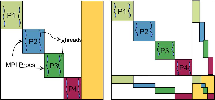
(a) Narrow Separator. (b) Wide Separator.
Figure 2. Wide Separator and Narrow Separator of a graph G.
use wide separators for increased parallelism. Note that the
Schur complement using the wide separator is similar to the
Ŝ11 = Ĝ11 − R̂11 ∗ D̂1−1 ∗ Ĉ11 + R̂12 ∗ D̂2−1 ∗ Ĉ21 (4) local Schur complement [17].
Computing the Schur complement in the above form is The edge separator from graph and hypergraph parti-
expensive due to the communication involved. However, the tioning gives a wide (vertex) separator by simply taking
doubly bordered block diagonal form for two parts when the boundary vertices. Although this is a good approach
we use a wide separator has more structure to it as shown for most problems, we observed that on problems with a
below. few dense rows or columns, the narrow separator approach
works better. Therefore, ShyLU also has the option to use
D11 0 C11 0
0 narrow separators. While some partitioners can compute
D22 0 C22
Awide = R11
(5) narrow vertex separators directly, we implemented a simple
0 G11 G12
heuristic to compute a (narrow) vertex separator from the
0 R22 G21 G22
edge separator so we can use any partitioner.
Although this block partition is similar to Equation (3),
the matrix blocks will in general have different sizes since IV. I MPLEMENTATION
a wide separator is larger than the corresponding narrow This section describes the implementation details of
separator. Consider that rows of Dii are the interior vertices ShyLU for each step of the Schur complement framework.
in part i and the rows in Rij are boundary vertices in part ShyLU uses an MPI and threads hybrid programming model
i then we observe that all blocks Rij and Cij will be equal even within the node. Notice that in the Schur complement
to zero when i 6= j. This follows from the definition of the framework the partitioning and reordering is purely alge-
wide separator. braic. This reordering exposes one level of data parallelism.
As R and C are block diagonal matrices, we can compute ShyLU uses MPI tasks to solve for each Di and the Schur
the Schur complement without any communication. For complement. A further opportunity for parallelism, is within
example, to compute the S11 block of the Schur complement the diagonal blocks Di . where a threaded direct solver, for
of Awide we do example, Pardiso [7] or SuperLU-MT [5], [6], is used to
factor each block Di . The assumption here is multithreaded
S11 = G11 − R11 ∗ D1−1 ∗ C11 (6)
direct solvers (or potentially incomplete factorizations in
Thus computing S in the wide separator case is fully the future) can scale well within a uniform memory access
parallel. The off-diagonal blocks of the Schur complement (UMA) region, where all cores have equal (fast) access to
are equal to the off-diagonal blocks of G. However, the a shared memory region. Using MPI between UMA regions
wide separator can be as much as two times the size of the mitigates the problems with data placement and non-uniform
narrow separator. This results in a larger Schur complement memory accesses and also allows us to run across nodes, if
system to be solved when using the wide separator. When the desired.
separator was considered as a serial bottleneck (when they ShyLU uses the Epetra package in Trilinos with MPI for
were originally designed for direct solvers) there was a good the matrix A. When combined with a multithreaded solver
argument to use the narrow separators. However, in hybrid for the subproblems, we have a hybrid MPI-threads solver.
solvers, we solve the Schur complement system in parallel This is a very flexible design that allows us to experiment
as well. As a result, while the bigger Schur complement with hybrid programming and the trade-offs of MPI vs.
system leads to increased solve time, the much faster setup threads. In the one extreme case, the solver could partition
due to increased parallelism offsets the small increase in and use MPI for all the cores and use no threads. The
solve time. All the experiments in the rest of this work other extreme case is to only use the multithreaded directsolver. We expect the best performance to lie somewhere in We choose to use a sparse direct solver. All the results in
between. A reasonable choice is to partition for the number Section VI use Pardiso [7] from Intel MKL, which is a
of sockets or UMA regions. We will study this in Section VI. multithreaded solver. Since the direct solver typically will
The framework consists of partitioning, sparse approxi- run within a single UMA region, it does not need to be
mation of the Schur complement, and fast, inexact (or exact) NUMA-aware. ShyLU uses the Amesos package [22] in
solution of the Schur complement. The first two steps only Trilinos which is a common interface to multiple direct
have to be done once in the setup phase. solvers. This enables ShyLU to switch between any direct
solver supported by the Amesos package. The other hybrid
A. Partitioning solvers mentioned in Section I all use a serial direct solver
ShyLU uses graph or hypergraph partitioning to find a D in this step.
that has a block structure and is suitable for parallel solution.
C. Approximations to the Schur Complement
To exploit locality (on the node), we partition A into k parts,
where k > 1 may be chosen to correspond to number of The exact Schur complement is S = G − R ∗ D−1 C.
cores, sockets, or UMA regions. The partitioning induces In general, S can be quite dense and is too expensive to
the following block structure: store. There are two ways around this: First, we can use S
implicitly as an operator without ever forming S. Second,
D C we can form and store a sparse approximation S̄ ≈ S. As
A= , (7)
R G we will see, both approaches are useful.
where D again has a block structure. As shown in Figure 1 The Schur complement itself has a block structure
there are two cases. In the symmetric case, ShyLU uses
S11 S12 . . . S1k
a symmetric permutation P AP T to get a doubly bordered S21 S22 . . . S2k
S= . (8)
block form. In this case, D = diag(D1 , . . . , Dk ) is a block .. ..
.. . .
diagonal matrix, R is a row border, and C is a column
border. In the nonsymmetric case, there is no symmetry to Sk1 Sk2 ... Skk
preserve so we allow nonsymmetric permutations. There- where it is known that the diagonal blocks Sii are usually
fore, instead we find P AQ with a singly bordered block quite dense but the off-diagonal blocks are mostly sparse
diagonal form (Figure 1(b)). A difficulty here is that the [17]. Note that the local Schur complements Sii can be
−1
“diagonal” blocks are rectangular, but we can factor square computed locally by Sii = Gii − Ri ∗ Dii Ci . A popular
submatrices of full rank and form R, the row border after choice is therefore to use the local Schur complements as a
the factorization. ShyLU can use a direct factorization that block diagonal approximation. As we use wide separators as
can factor square subblocks of rectangular matrices. There discussed above all the fill is in our local Schur complement
are no multithreaded direct solvers that can handle this case and all the offdiagonal blocks have the same sparsity pattern
now. We focus on the structurally symmetric case here. In as the corresponding Gij . To save storage, the local Schur
our experiments for unsymmetric matrices, we apply the complements themselves need to be sparsified [23], [15].
permutation in a symmetric manner to form the DBBD form. We investigate two different ways to form S̄ ≈ S:
Several variations of graph partitioning can be used to ob- Dropping and Probing. Both methods attempt to form a
tain block bordered structure. Traditional graph partitioning sparser version of S while preserving the main properties
attempts to keep the parts of equal size while minimizing of S.
the edge cut. We will consider the edge separator as our sep- 1) Dropping (value-based): With dropping we only keep
arator. The other hybrid solvers we know (see Section I) use the largest (in magnitude) entries of S. This is a common
some form of graph partitioning. Hypergraph partitioning is strategy and was also used in HIPS and PDSLin. Symmetric
a generalization of graph partitioning that is also well suited dropping is used in [24]. When forming S = G−R∗D−1 C,
for our problem because it can minimize the border size we simply drop entries less than a given threshold. We use a
directly. Also, it naturally handles nonsymmetric problems, relative threshold, dropping entries that are smaller relative
while graph partitioning requires symmetry. ShyLU uses to the large entries. Since S can be quite dense, we only form
hypergraph partitioning in both the symmetric and nonsym- a few columns at a time and immediately sparsify. Note we
metric cases. ShyLU uses the Zoltan/PHG partitioner [21] do not drop entries based on U −1 C or R∗U −1 where L and
and computes the wide separators and narrow separators U are the LU factors of D, as in HIPS or PDSLin. Since
from a distributed matrix. our dropping is based on the actual entries in S, we believe
our approximation S̄ is more robust. However, even with
B. Diagonal block solver the parallelism at the MPI level, computing local Sii to drop
The blocks Di are relatively small and will typically the entries is itself expensive. Instead of trying to parallelize
−1
be solved on a small number of cores, say in one UMA the sparse triangular solve to compute the Rii ∗ Dii ∗ Cii ,
region. Either exact or incomplete factorization can be used. we compute the columns of S in chunks and exploit the(a) Structure of typical banded probing for S̄, B. (b) Structure of G submatrix. (c) Structure of S̄ = B∪G for ShyLU’s probing.
Figure 3. A sketch of the pattern used for probing in ShyLU.
parallelism available from using the multiple right hand sides are
in a sparse triangular solve.
1 0 0
0 1 0
0 0 1
V = 1 (9)
2) Probing (structure-based): Since dropping may be 0 0
expensive in some cases, ShyLU can also use probing. 0 1 0
.. .. ..
Probing was developed to approximate interfaces in domain
. . .
decomposition [25], which is also a Schur complement. In
probing, we select the sparsity pattern of S̄ ≈ S first. Given with Vij = 1 if column i had color j. S ∗ V gives us
a sparsity pattern we probe the Schur complement operator the entries corresponding to the tridiagonal of the Schur
S for the entries given in the sparsity pattern instead of complement in a packed format. However, a purely banded
computing the entire Schur complement and drop the entries. approximation will lose any entries in S (and G) that are
It is possible to probe the operator efficiently by coloring the outside the bandwidth. To strengthen our preconditioner, we
sparsity pattern of S̄ and computing a set of probing vectors, include the pattern of G in the probing pattern, which is
V , based on the coloring of S̄. V is a n-by-k matrix where simple to do as G is known a priori. To summarize, the
k is the number of colors and n is the dimension of S. The pattern of S̄ in ShyLU’s probing is pattern of B ∪ G, where
number of colors in the coloring problem corresponds to B is a banded matrix.
the number of probing vectors needed. The coloring of the Figure 3 shows a sketch of how ShyLU’s probing tech-
pattern computes the orthogonal columns in S̄, so we apply nique compares to traditional probing. Figure 3(a) shows
the operator to only the few vectors that are needed. the structure of a typical banded probing assuming we are
looking for a few diagonals. To this structure, our algorithm
also includes the structure of G from the reordered matrix
Finally, we apply S = G − RD−1 C as an operator to
(Figure 3(b)), for probing. As result the structure for the
the probing vectors V to obtain SV , which then gives us
probing is as shown in Figure 3(c). The idea behind adding
the numerical values for S̄ in a packed format. We need to
G to the structure of S̄ is that any entry that is originally
unpack the entries to compute S̄. We refer to Chan et al. [25]
part of G is important in S̄ as well. Experimental results
for the probing algorithm.
showed a bandwidth of 5% seems to work well for most
problems.
Generally, the sparser S̄, the fewer the number of probing Probing for a band structure is straight-forward since the
vectors needed. Choosing the sparsity pattern of S̄ can be probing vectors are trivial to compute. In our approach, we
tricky. For PDE problems where the values in S decay away need to use graph coloring on the structure of S̄ (which
from the diagonal, a band matrix is often used [25]. We in our case is B ∪ G) to find the probing vectors. We use
show how probing works by using a tridiagonal approxima- the Prober in Isorropia package of Trilinos which in turn
tion of the Schur complement as an example. Coloring the uses the distributed graph coloring algorithm [26] in Zoltan.
pattern of a tridiagonal matrix results in three colors. Then Note that all the steps in probing - the coloring, applying the
the three probing vectors corresponding to the three colors probing vector and extracting S̄, are done in parallel. Probingfor a complex structure is computationally expensive, but we The block diagonal solvers are multithreaded in addition to
save quite a lot in memory as the storage required for the the parallelism from the MPI level. We use parallel coloring
Schur complement is the size of G with a few diagonals. from Zoltan to find orthogonal columns in the structure of
However, for problems where the above discussed structure S̄ and sparse matrix vector multiplication to do the probing.
of S̄ is not sufficient, the more expensive dropping strategy The Schur complement solve uses our parallel iterative
can be used. solvers for solving for S or S̄ which use a multithreaded
matrix vector multiplication.
D. Solving for the Schur Complement
V. PARALLEL N ODE L EVEL P RECONDITIONING
As in the steps before, there are several options for solving
for the Schur complement as well. Recall that we have ShyLU is a hybrid solver designed for the multicore node
formed S̄, a sparse approximation to S. A popular approach and uses MPI and threads even within the node. This is
in hybrid methods is to solve the Schur complement system different from other approaches where MPI + threads model
iteratively using S̄ as a preconditioner. In each iteration, we spans across the entire system, not just the node, and there
have to apply S, which can be done implicitly without ever is only one MPI processes per node. We see two problems
forming S explicitly. Note that implicit S requires sparse with one MPI process per node approach:
triangular solves for D in every iteration. We call this the 1) Parts of the applications other than the solver have
exact Schur complement solver. fewer MPI processes limiting their scalability.
As we only need an inexact solve as a preconditioner, 2) Scaling the multithreaded solvers on the compute
it is also possible to solve S̄ instead of solving S. Now, nodes with NUMA accesses is a harder problem.
even S̄ is large enough that it should be solved in parallel. Instead, we believe one MPI process per socket or UMA
We solve for S̄ iteratively using yet another approximation region is a more practical approach for scalability at least
S̃ ≈ S̄ as a preconditioner for S̄. It should be easy to solve in the near term. ShyLU also decouples the idea that
for S̃ in parallel. In practice, S̃ can be quite simple, for one subdomain corresponds to one MPI process. An MPI
example, diagonal (Jacobi) or block diagonal (block Jacobi). based subdomain solver like ShyLU allows the subdomain,
The main difference from the exact method is that we do in a domain decomposition method, to span several MPI
not use the Schur complement operator even for matrix processes.
vector multiplies in the inner iteration. Instead we use S̄. Nothing prevents us from using ShyLU across the entire
We call this approach the inexact Schur complement solver. system as it is based on MPI, however the separator size (and
ShyLU can do both the exact and inexact solve for the thus the Schur complement) will grow with the number of
Schur complement. We compare the robustness of both these parts. While using a multithreaded solver for the D blocks
approaches in Section VI. limit the size of the Schur complement to a certain extent
Once the preconditioner (S̄ or S̃) and the operator for (by partitioning for fewer MPI processes) we recommend
our solve (either an implicit S or S̄) is decided there are using a domain decomposition method with little commu-
two options for the solver. If D is solved exactly and an nication (e.g., additive Schwarz) at the global level, and
implicit S is the operator it is sufficient to iterate over S ShyLU on the subdomains. Such a scheme will exploit
(as in [13]) and not on A. Instead any scheme that uses an three levels of parallelism, where the top level requires
inexact solve for D or an iterative solve on S̄ (instead of little communication while the lower levels require more
S) or both implies an inner-outer iterative method for the and more communication. In essence, we adapt the solver
overall system. as it is required to iterate on A. It is because algorithm to the machine architecture. We believe this is
of this reason ShyLU uses an inner-outer iteration, where a good design for future exascale computers that will be
the inner iteration is only on the Schur complement part. hierarchical in structure.
The inner iteration (over S or S̄) is internal in the solver The Schur complement framework and the MPI+threads
and invisible to the user, while the outer iteration (over A) programming model also allow ShyLU be fully flexible in
is controlled by the user. We expect a trade-off between the terms of how applications use it. We envision ShyLU to be
inner and outer iterations. That is, if we iterate over S we used by the applications in three different modes:
need few outer iterations while if we iterate on S̄ we may 1) When applications start one MPI process per UMA
need more outer iterations but fewer inner iterations. region in the near future, a simple MPI Comm Split()
By default, we do 30 inner iterations or to an accuracy of can map all the MPI processes in a node to ShyLU’s
10−10 whichever comes first. MPI processes. A subdomain will be defined as one
per node.
E. Parallelism 2) When applications start one MPI process per node,
Our implementation of the Schur complement framework additive Schwarz will use a threads-only ShyLU.
is parallel in all three steps. We use Zoltan’s parallel hy- 3) Applications that now run one MPI process per core
pergraph partitioning to partition and reorder the problem. remain that way, the additive Schwarz preconditionerbecause of its NUMA properties. The 24 cores in a node
are in fact four six-core UMA sets. We use Hopper for
all our strong scaling and weak scaling studies. Our other
test platform is an eight-core (dual-socket quad-core) Linux
workstation that represents current multicore systems. We
use this workstation for our robustness experiments.
All experimental results show the product of inner and
outer iterations that will be seen by the user of ShyLU.
When there are many tunable parameters there are two
ways to do experiments. Either choose the best parameters
for each problem, or always use the same parameters for
a given solver on the entire test set. All the experiments
in this section use solver specific parameters and there is
no tuning for a particular problem, since this is how users
typically use software. For probing we add 5% of diagonals
to the structure of G. For dropping, our relative dropping
Figure 4. Cross-section of 3D unstructured mesh on an irregular domain. threshold is 10−3 . We use 30 inner iterations or 10−7 relative
residual whichever comes first and 500 outer iterations or
10−7 relative residual whichever comes first. This is fully
(which will use ShyLU on subdomains) can define the utilized when we use the inexact Schur complement.
subdomains as one per node and transform the matrix
for ShyLU. ShyLU will not be able to use additional B. Robustness
threads in this case. We validate the different methods in ShyLU by com-
Thus the MPI+threads programming model in ShyLU’s paring it to incomplete factorizations and the HIPS [13]
design helps make the application migration to the multicore hybrid solver. We use three different variations of ShyLU,
systems smooth depending on how the applications want to approximations based on dropping and probing with the
migrate. exact Schur complement solver and approximations based on
dropping and the inexact Schur complement solver. All three
VI. R ESULTS approaches have tunable parameters that can be difficult
We perform three different set of experiments. First, we to choose. We used a fixed dropping/probing tolerance in
wish to test robustness of ShyLU compared to other common all our tests. The relative threshold for dropping is 10−3 .
algebraic preconditioners. Second, we study ShyLU perfor- Similarly, we tested HIPS preconditioner with fixed settings
mance on multicore platforms, and in particular the trade-off same as ShyLU. Our goal is to demonstrate the robustness
between MPI-only vs. hybrid models. This study will also of ShyLU compared to one other hybrid solver that is
look at performance of ShyLU while doing strong scaling. commonly used today. The tests also include ILU with
Third, we study weak scaling of ShyLU on both 2D and 3D one level of fill. The number of iterations of the three
problems. methods should not be compared directly, since the fill and
work differ in the various cases. The methods can be made
A. Experimental setup
comparable by tuning the knobs. However, we have used the
We have implemented ShyLU in C++ within the Trili- parameters as they are used in our various applications.
nos [3] framework. We leverage several Trilinos packages, We chose nine sparse matrices from a variety of appli-
in particular: cation areas, taken from the University of Florida sparse
1) Epetra for matrix and vector data structures and ker- matrix collection [27]. We added one test matrix from a
nels. Sandia application, TC N 360K. The results are shown in
2) Isorropia and Zoltan for matrix partitioning and prob- Table I. We see that the dropping approximation with the
ing. exact Schur complement is the most robust approach among
3) AztecOO and Belos for iterative solves (GMRES). all the approaches, in the sense it has fewer failures. This has
In addition to the Trilinos packages we also use PARDISO been observed in the past by others as well. The dropping
as our multithreaded direct solver. We use two test platforms. with exact Schur complement is better or very close to
The first is Hopper, a Cray XE6 at NERSC. Hopper has HIPS in terms of the number of iterations. Generally, the
6392 nodes, each with two twelve-core AMD MagnyCours drop-tolerance version requires fewer iterations (though not
processors running at 2.1 GHz. Thus, each node has 24 necessarily less run time) than the probing version.
cores and is a reasonable prototype for future multicore A dash indicates that GMRES failed to converge to the
nodes. Furthermore, the Hopper system is attractive to us desired tolerance within 500 iterations. Note that the circuitMatrix Name N Symmetry ShyLU Dropping ShyLU Probing ShyLU Dropping HIPS ILU
Exact Schur Exact Schur Inexact Schur
venkat50 62.4K Unsymmetric 12 76 - 8 374
TC N 360K 360K Symmetric 32 82 17 19 203
Pres Poisson 14.8K Symmetric 14 26 14 11 -
FEM 3D thermal2 147K Unsymmetric 3 6 3 3 20
bodyy5 18K Symmetric 3 5 3 3 120
Lourakis bundle1 10K Symmetric 7 18 7 10 26
af shell3 504K Symmetric 50 - 39 29 -
Hamm/bcircuit 68.9K Unsymmetric 6 6 4 42 -
Freescale/transient 178.8K Unsymmetric 88 - - 440 -
Sandia/ASIC 680ks 682K Unsymmetric 4 34 2 2 57
Table I
C OMPARISON OF NUMBER OF ITERATIONS OF S HY LU DROPPING AND PROBING WITH EXACT SOLVE , S HY LU DROPPING WITH INEXACT SOLVE , HIPS
AND ILU(1) FOR MATRICES FROM UF COLLECTION . A DASH INDICATES NO CONVERGENCE .
MPI Processes x Number of Threads in
matrices bcircuit and transient are difficult for HIPS, but each node
ShyLU does well in these matrices. The matrix af shell3 Nodes 4x6 6x4 12x2 24x1
has been called horror matrix in the past for posing difficulty (Cores)
1 (24) 19.6 ( 79) 17.9 ( 91) 11.8 (122) 8.3 (144)
to preconditioners. Both ShyLU and HIPS could solve this 2 (48) 14.6 (115) 12.3 (122) 7.0 (144) 6.9 (196)
problem easily. ILU(1) does poorly on all the problems when 4 (96) 8.3 (122) 7.2 (144) 5.3 (196) 6.0 (227)
compared with the two hybrid preconditioners. However, 8 (192) 6.4(176) 5.2(196) 3.9(227) 6.9 (332)
that is expected given the fact that ILU(1) uses considerably Table II
less memory and has little information in the preconditioner S TRONG S CALING AND H YBRID VS MPI- ONLY PERFORMANCE : S OLVE
TIME IN SECONDS (# ITERATIONS ) FOR S HY LU DROPPING METHOD TO
itself. SOLVE A LINEAR SYSTEM OF SIZE 360 K .
We further observe that the dropping version is more
robust than the probing version, as it solved all 10 test prob-
lems while the probing version failed in 2 out of 10 cases.
The inexact approach, as one would expect, is not as robust the performance figures for more than 24 cores to get better.
as the exact approach with dropping. However, it converged However, we do not know how much MPI and threads
faster when it worked. We have also verified that ShyLU performance are going to get better. Assuming they improve
takes less memory than a direct solver UMFPACK [28]. The at the same rate, we compare the performance of the MPI-
amount of memory used by ShyLU depends on the size of only code with hybrid code to understand the possible
the Schur complement, dropping criterion, and the solver differences in future systems.
used for the block diagonals.
For this experiment we used a 3D finite element dis-
C. MPI+threads vs MPI performance cretization of Poisson’s equation on an irregular domain,
We implemented ShyLU with MPI at the top level. Each shown in Figure 4. The matrix dimension was 360K. We
MPI process corresponds to a diagonal block Di . We used use the drop-tolerance version of ShyLU for our first set of
multi-threaded MKL-Pardiso as the solver for the Di blocks. tests. For each node with 24 cores, we tested the following
We wish to study the trade-off between MPI-only and hybrid configurations of MPI processes × threads: 4 × 6, 6 × 4,
models. Our design allows us to run any combination of MPI 12 × 2, and 24 × 1. The results for run-time and iterations
processes and threads. Note that when we vary the number of are shown in Table II. More than 6 threads per node is not
MPI processes, we also change the number of Di blocks so a recommended configuration for Hopper so those results
the preconditioner changes as well. Thus, what we observe in are not shown in Table II. The solve time is also shown in
the performance is a combined effect of changes in the solver Figure 5(a).
algorithm and in the programming model (MPI+threads). There are several interesting observations. First, we see
Initially, we ran on one node of Hopper (24 cores). that although the number of iterations increase with the
However, the number of cores on a node is increasing number of MPI processes (going across the rows in Table II),
rapidly. We want to predict performance on future multicore the run times may actually decrease. On a single node, we
platforms with hundreds of cores. We simulate this by see that the all-MPI version (24x1) is fastest, even though
running ShyLU on several compute nodes. Since we use it uses more iterations.
MPI even within the node, ShyLU also works across nodes. Second, we see that, as we add more nodes, the run times
We expect future multicore platforms to be hierarchical with decrease much more rapidly for the hybrid configurations.
highly non-uniform memory access and running across the For example, with four nodes, the 12x2 configuration gives
nodes will reasonably simulate future systems. We expect the fastest solve time. This is good news for hybrid methods(a) Dropping (b) Probing
Figure 5. Strong Scaling: ShyLU’s dropping and probing methods for a matrix of size 360K. Solve Time shown for MPI tasks x Threads.
MPI Processes x Number of Threads in
each node The number of iterations for this experiment is shown in
Nodes 4x6 6x4 12x2 24x1 Table III. We can see that the number of iterations for the
(Cores) probing method is better than the dropping method.
1 (24) 17.1 ( 64) 15.4 ( 70) 9.4 ( 83) 8.7 ( 97)
2 (48) 13.7 ( 76) 9.7 ( 83) 6.7 ( 97) 6.3 (114)
To verify our conjecture, that the size of the problem in
4 (96) 8.8 ( 98) 6.3 ( 97) 4.8 (114) 6.9 (148) each subdomain is important for hybrid performance, we
8 (192) 5.7 (111) 4.6 (114) 4.5(148) 9.3 (218) repeated the experiment, this time with a larger problem
Table III 720Kx720K. We did not use the 4x6 configuration as it
S TRONG SCALING AND H YBRID VS MPI- ONLY PERFORMANCE : S OLVE was the slowest in our previous experiment. The results are
TIME IN SECONDS (# ITERATIONS ) FOR S HY LU PROBING METHOD TO
SOLVE A LINEAR SYSTEM OF SIZE 360 K .
shown in Table IV. Note that ShyLU scales well up to 384
cores. Furthermore, we see that the crossover point where
MPI+threads beats MPI-only implementation is different for
MPI Processes x Number of Threads in this larger problem (384 cores). The result can be seen
each node clearly in Figure 6 where we compare the 12x2 case against
Nodes 6x4 12x2 24x1 24x1 for both the problems (360K and 720K). When the
(Cores)
2 ( 48) 25.1( 90) 15.0(104) 11.5(115) problem size per subdomain is about 3500 unknowns the
4 ( 96) 13.8(104) 9.2(115) 6.2(130) performance is almost the same for all four cases. As
8 (192) 9.5(115) 5.7(130) 5.1(139) the problem size per subdomain gets smaller the hybrid
16 (384) 5.1(130) 3.2(139) 4.8(177)
programming model gets better.
Table IV A consistent trend in our results is that as the number
S TRONG SCALING AND H YBRID VS MPI- ONLY PERFORMANCE : S OLVE
TIME IN SECONDS (# ITERATIONS ) FOR S HY LU DROPPING METHOD TO of cores increase, and the size of the problems get smaller,
SOLVE A LINEAR SYSTEM OF SIZE 720 K . the hybrid (MPI+threads) solver outperforms the MPI-only
based solver.
D. Strong scaling
as they can take advantage of the node level concurrency. We We can also get strong scaling results by looking at a
believe that this is mainly due to the subproblems getting column at a time at the Tables II – IV. In the 360K
smaller. We conjecture that using more threads would be problem’s dropping case, the 4 × 6 configuration gives a
helpful on smaller problem sizes per core. speedup of 2.3 going from one to four nodes, while the
To understand how the algorithmic choices affect our 24×1 only gave a speedup of 1.4. Although the first is quite
strong scaling results we also repeated the experiment with decent when one takes the communication across nodes into
the same 360Kx360K problem with probing. The time for account, one should keep in mind that ShyLU was primarily
the solve is shown in Figure 5(b). The results are almost intended to be a fast solver on a single node. The results are
identical to the dropping method. The MPI only version similar when we go to eight nodes (192 cores). The best
started performing poorly at 96 cores. At 192 cores any speedup the hybrid model achieved is 3.4 while MPI-only
MPI+thread combination beats MPI-only implementation. is able to get a speedup of 1.2 for the dropping method. The
However, MPI only is still the best choice at 24 cores. 6x4 and 12x2 configurations in the 720K problem size caseMPI Processes x Number of Threads in
each node
Nodes 4x6 6x4 12x2 24x1
(Problem Size)
1 (60K) 0.37(17) 0.31(18) 0.20(22) 0.39(27)
2 (120K) 0.48(20) 0.51(26) 0.30(27) 0.50(30)
4 (240K) 0.82(29) 0.49(25) 0.38(28) 0.44(31)
8 (480K) 0.83(29) 0.66(30) 0.44(30) 0.55(32)
Table VI
S HY LU ( DROPPING ) WEAK SCALING RESULTS : T IMING IN SECONDS
(# ITERATIONS ) FOR 2D FINITE ELEMENT PROBLEM .
MPI Processes x Number of Threads in
each node
Nodes 4x6 6x4 12x2 24x1
(Problem)
(Size)
1 (90K) 3.0(47) 2.53(54) 1.76(67) 1.37(73)
2 (180K) 4.55(71) 3.93(80) 2.78(95) 2.41(110)
Figure 6. Solve time for MPI-only and MPI+threads implementations for
4 (360K) 8.34(122) 7.25(144) 5.31(196) 6.09(227)
different problem sizes per subdomain.
8 (720K) 10.30(103) 9.59(115) 5.78(130) 5.17(139)
MPI Processes x Number of Threads in Table VII
each node S HY LU ( DROPPING ) WEAK SCALING RESULTS : T IMING IN SECONDS
Nodes 4x6 6x4 12x2 24x1 (# ITERATIONS ) FOR THE 3D PROBLEM .
(Problem Size)
1 (60K) 0.25(10) 0.19(10) 0.35(26) 0.21(11)
2 (120K) 0.31(11) 0.22(10) 0.40(26) 0.61(26)
4 (240K) 0.33(11) 0.67(26) 0.20(12) 0.74(26)
8 (480K) 0.41(11) 0.29(11) 0.60(26) 0.82(26) coefficients, generated in Matlab by the command
Table V
A = gallery(’wathen’,nx,ny). We vary the num-
S HY LU ( PROBING ) WEAK SCALING RESULTS : T IMING IN SECONDS ber of nodes from one to eight. Again, we designed ShyLU
(# ITERATIONS ) FOR 2D FINITE ELEMENT PROBLEM . to be run within a node but we want to demonstrate scaling
beyond 24 cores, so we run our experiments across multiple
nodes.
We see in Tables V– VI that both run time and number of
(Table IV) achieve a speed up of 4.92 and 4.68 going from iterations increase slowly with the number of cores (as we
48 to 384 cores. MPI-only implementation gained a speedup go down the columns). The dropping version demonstrates a
of 2.39 for this case. Overall, ShyLU is able to scale up to smooth and predictable behavior, while the probing version
384 cores reasonably well. has sudden jumps in number of iterations and time. We
One should also note that the MPI+threads approach has conjecture that this is because the preconditioner is sensitive
allowed us to reduce the iteration creep that we would to the probing pattern (which is difficult to choose). For
expect to see in many precondtioners as the problem size the dropping version, the 12x2 configuration with 12 MPI
and number of processes increase. For example, in Table II, processes and 2 threads each per node is consistently the
we can see that the configuration of 8 nodes with 12 MPI best.
processes and 2 threads in each node and the configuration Our 3D test problem is a finite element discretization of an
of 4 nodes with 24 MPI processes (1 thread in each process) elliptic PDE on the unstructured grid show in Figure 4. The
gives us the same number of iterations – 227. However, the weak scaling results for this problem are shown in Table VII.
former is using the two threads for better scalability and We observe that going from 1 to 8 nodes, the number of
takes only 65% of the time. iterations roughly doubles while the run time roughly triples.
Although worse than the optimal O(n) scaling that multigrid
E. Weak scaling methods may be able to achieve, this is much better than the
We perform weak scaling experiments on both 2D and 3D typical O(n2 ) operations scaling by general sparse direct
problems where we keep the number of degrees of freedom solvers. ShyLU’s intended usage as a subdomain solver
(matrix rows) per core constant. This is not the intended also places more emphasis on strong scaling than weak
use case for ShyLU (as a subdomain solver, strong scaling scaling, as the problem size per node is not growing as
is more relevant) but we wish to show that ShyLU also does fast as the node concurrency. We conclude that ShyLU is
reasonably well in this setting. a good subdomain solver for problems of moderate size and
Our 2D test problem is a finite element discretization scales quite well up to 384 cores. Thus, it can also be used
of an elliptic PDE on a structured grid but with random as a solver/preconditioner in itself on such problems andplatforms. VIII. C ONCLUSIONS
VII. F UTURE W ORK We have introduced a new hybrid-hybrid solver, ShyLU.
ShyLU is hybrid both in the mathematical sense (direct
We plan several improvements in ShyLU. Some of these and iterative) and in the parallel computing sense (MPI
deal with combinatorial issues in the solver algorithm, others + threads). ShyLU is both a robust linear solver and a
are numerical. flexible framework that allows researchers to experiment
First, we wish to further study the partitioning and or- with algorithmic options. We introduced and explored sev-
dering strategy. In concurrent work [29] we explored the eral such options: a new probing based Schur complement
trade-off between load imbalance in the diagonal blocks approximation vs. the traditional dropping strategy, wide vs.
and the size of the Schur complement. By allowing more narrow separators, and exact vs. inexact solves for the Schur
imbalance in the diagonal blocks, the partitioner can usually complement system. Performance results show ShyLU can
find a smaller block border. We have also observed that scale well for up to 384 cores in the hybrid mode.
the load balance in the system for the inner solve (S) We also studied the question, that given a complex algo-
may be poor even though the load balance for the outer rithm, with a MPI-only implementation and hybrid (MPI
problem (A) is good. With current partitioning tools one can +Threads) implementation, for a fixed set of parameters:
balance the interior vertices but not the work in the sparse Can the hybrid implementation beat the MPI-only imple-
factorization or solve. Furthermore, it is not sufficient to mentation? Empirical results on a 24-core MagnyCours node
balance the interior vertices (or factorization work) because show that it is advantageous to run MPI on the node.
ShyLU would require the boundary vertices to be balanced This is not surprising since MPI gives good locality and
as well as that corresponds to the number of triangular memory affinity. However, we project that for applications
solves and matrix vector multiplies while constructing the and algorithms with smaller problem size per domain, MPI-
Schur complement. We believe this issue poses a partitioning only works well up to about 48 cores, but for 96 or more
problem with multiple constraints and objectives, and cannot cores hybrid methods are faster. The crossover point where
be adequately handled using standard partitioning models. the hybrid model beats MPI depends on the problem size per
Second, we intend to extend the code to handle struc- subdomain. We conclude that MPI-only solvers is a good
turally nonsymmetric problems with nonsymmetric permu- choice for today’s multicore architectures. However, consid-
tations. Our current implementation uses symmetric ordering ering the fact that the number of cores per node is increasing
and partitioning, even for nonsymmetric problems. We can steadily and memory architectures are changing to favor
use the hypergraph partitioning and permutation to singly core-to-core data sharing, hybrid (hierarchical) algorithms
bordered block form as shown in Figure 1. However, this and implementations are important for future multicore
requires a multithreaded direct solver that can handle rect- architectures. We predict multiple levels of parallelism will
angular blocks. be essential on future exascale computers.
Third, one could study the effect of inexact solves (e.g.,
with incomplete factorizations) on the diagonal blocks (Di ). ACKNOWLEDGMENT
This will require the iterative solver to iterate on the entire Sandia is a multiprogram laboratory operated by Sandia
system, not just the Schur complement. The number of Corporation, a wholly owned subsidiary of Lockheed Mar-
iterations will likely increase, but both the setup and each tin, for the United States Department of Energy’s National
solve on the diagonal blocks will be faster. This variation Nuclear Security Administration under contract DE-AC04-
would also need less memory. 94AL85000.
Fourth, we should test ShyLU on highly ill-conditioned The authors thank the Department of Energy’s Office
problems, such as indefinite problems and systems from of Science and the Advanced Scientific Computing Re-
vector PDEs. Although ShyLU is robust on the range of search (ASCR) office for financial support. This research
problems we tested here, harder test problems may reveal used resources of the National Energy Research Scientific
the need for some algorithmic adjustments. Computing Center (NERSC), which is supported by the
Finally, we plan to integrate ShyLU as a subdomain Office of Science of the DOE under Contract No. DE-AC02-
solver within a parallel domain decomposition framework. 05CH11231.
This would comprise a truely hierarchical solver with three
different layers of parallelism in the solver. R EFERENCES
We remark that none of these issues are specific to ShyLU [1] M. Gee, C. Siefert, J. Hu, R. Tuminaro, and M. Sala, “ML
and many also apply to other hybrid solvers. Discussions 5.0 smoothed aggregation user’s guide,” Sandia National
with developers of other such solvers have confirmed that Laboratories, Tech. Rep. SAND2006-2649, 2006.
they face similar issues. In particular, we believe research [2] R. D. Falgout and U. M. Yang, “Hypre: A library of high
on the combinatorial problems above may help advance a performance preconditioners,” Lecture Notes in Computer
whole class of solvers. Science, vol. 2331, pp. 632–??, 2002.[3] M. A. Heroux, R. A. Bartlett, V. E. Howle, R. J. Hoekstra, [16] Y. Saad and M. Sosonkina, “Distributed Schur complement
J. J. Hu, T. G. Kolda, R. B. Lehoucq, K. R. Long, R. P. techniques for general sparse linear systems,” SIAM J. Sci.
Pawlowski, E. T. Phipps, A. G. Salinger, H. K. Thornquist, Comput, vol. 21, pp. 1337–1356, 1997.
R. S. Tuminaro, J. M. Willenbring, A. Williams, and K. S.
Stanley, “An overview of the Trilinos project,” ACM Trans. [17] Y. Saad, Iterative Methods for Sparse Linear Systems, 2nd ed.
Math. Softw., vol. 31, no. 3, pp. 397–423, 2005. SIAM, 2003.
[4] S. Balay, W. D. Gropp, L. C. McInnes, and B. F. Smith, Effi- [18] M. Sala and M. Heroux, “Robust algebraic preconditioners
cient management of parallelism in object-oriented numerical with IFPACK 3.0,” Sandia National Laboratories, Tech. Rep.
software libraries. Birkhauser Boston Inc., 1997, pp. 163– SAND-0662, February 2005.
202.
[19] J. R. Gilbert and E. Zmijewski, “A parallel graph partitioning
[5] J. W. Demmel, J. R. Gilbert, and X. S. Li, “An asynchronous algorithm for a message-passing multiprocessor,” Interna-
parallel supernodal algorithm for sparse gaussian elimina- tional Journal of Parallel Programming, vol. 16, pp. 427–449,
tion,” SIAM J. Matrix Anal. Appl., vol. 20, pp. 915–952, July 1987.
1999.
[20] A. George, M. T. Heath, J. Liu, and E. Ng, “Sparse Cholesky
[6] X. S. Li, “An overview of SuperLU: Algorithms, implemen- factorization on a local-memory multiprocessor,” SIAM J. Sci.
tation, and user interface,” ACM Trans. Math. Softw., vol. 31, Stat. Comput., vol. 9, pp. 327–340, March 1988.
pp. 302–325, September 2005.
[21] K. Devine, E. Boman, R. Heaphy, R. Bisseling, and
[7] O. Schenk and K. Gärtner, “Solving unsymmetric sparse U. Catalyurek, “Parallel hypergraph partitioning for scientific
systems of linear equations with PARDISO,” Journal of computing,” in Proc. of 20th International Parallel and Dis-
Future Generation Computer Systems, vol. 20, no. 3, pp. 475– tributed Processing Symposium (IPDPS’06). IEEE, 2006.
487, 2004.
[22] M. Sala, K. S. Stanley, and M. A. Heroux, “On the design of
[8] P. Amestoy, I. Duff, J.-Y. L’Excellent, and J. Koster, MUl- interfaces to sparse direct solvers,” ACM Trans. Math. Softw.,
tifrontal Massively Parallel Solver (MUMPS Versions 4.3.1) vol. 34, pp. 9:1–9:22, March 2008.
Users’ Guide, 2003.
[23] L. Giraud, A. Haidar, and Y. Saad, “Sparse approximations
[9] P. R. Amestoy, I. S. Duff, J.-Y. L’Excellent, of the schur complement for parallel algebraic hybrid linear
and J. Koster, “MUMPS home page,” 2003, solvers in 3d,” Numerical Mathematics: Theory, Methods and
http://www.enseeiht.fr/lima/apo/MUMPS. Applications, vol. 3, no. 3, pp. 276–294, 2010.
[10] P. Henon, P. Ramet, and J. Roaman, “PaStiX: A parallel [24] E. Agullo, L. Giraud, A. Guermouche, and J. Roman, “Paral-
sparse direct solver based on a static scheduling for mixed lel hierarchical hybrid linear solvers for emerging computing
1d/2d block distributions,” in Proceedings of Irregular’2000, platforms,” Comptes Rendus Mecanique, vol. 339, pp. 96–
ser. Lecture Notes in Comput. Sci., S. Verlag, Ed., vol. 1800, 103, 2011.
2000, pp. 519–525.
[25] T. F. C. Chan and T. P. Mathew, “The interface probing
[11] D. Hysom and A. Pothen, “A scalable parallel algorithm for technique in domain decomposition,” SIAM J. Matrix Anal.
incomplete factorization,” SIAM J. on Sci. Comp., vol. 22, Appl., vol. 13, pp. 212–238, January 1992.
no. 6, pp. 2194–2215, 2001.
[26] D. Bozdağ, U. V. Çatalyürek, A. H. Gebremedhin, F. Manne,
E. G. Boman, and F. Özgüner, “Distributed-memory parallel
[12] J. I. Aliaga, M. Bollhöfer, A. F. Martı́n, and E. S. Quintana-
algorithms for distance-2 coloring and related problems in
Ortı́, “Exploiting thread-level parallelism in the iterative solu-
derivative computation,” SIAM J. Sci. Comput., vol. 32, pp.
tion of sparse linear systems,” Parallel Comput., vol. 37, pp.
2418–2446, August 2010.
183–202, March 2011.
[27] T. A. Davis and Y. Hu, “The Univerity of Florida collection,”
[13] J. Gaidamour and P. Henon, “A parallel direct/iterative solver
ACM Trans. Math. Software, vol. 38, no. 1, 2011.
based on a schur complement approach,” Computational
Science and Engineering, IEEE International Conference on,
[28] T. A. Davis, “Algorithm 832: UMFPACK v4.3—an
vol. 0, pp. 98–105, 2008.
unsymmetric-pattern multifrontal method,” ACM Trans. Math.
Softw., vol. 30, pp. 196–199, June 2004.
[14] L. Giraud and A. Haidar, “Parallel algebraic hybrid solvers
for large 3d convection-diffusion problems,” Numerical Algo- [29] E. G. Boman and S. Rajamanickam, “A study of combinato-
rithms, vol. 51, pp. 151–177, 2009. rial issues in a sparse hybrid solver,” in Proc. of SciDAC’11,
2011.
[15] I. Yamazaki and X. S. Li, “On techniques to improve ro-
bustness and scalability of a parallel hybrid linear solver,”
in Proceedings of the 9th international conference on High
performance computing for computational science, ser. VEC-
PAR’10. Berlin, Heidelberg: Springer-Verlag, 2011, pp. 421–
434.You can also read